Human activity modeling and Barabasi’s queueing systems

Abstract

It has been shown by A.-L. Barabasi that the priority based scheduling rules in single stage queuing systems (QS) generates fat tail behavior for the tasks waiting time distributions (WTD). Such fat tails are due to the waiting times of very low priority tasks which stay unserved almost forever as the task priority indices (PI) are ”frozen in time” (i.e. a task priority is assigned once for all to each incoming task). Relaxing the ”frozen in time” assumption, this paper studies the new dynamic behavior expected when the priority of each incoming tasks is time-dependent (i.e. ”aging mechanisms” are allowed). For two class of models, namely 1) a population type model with an age structure and 2) a QS with deadlines assigned to the incoming tasks which is operated under the ”earliest-deadline-first” policy, we are able to analytically extract some relevant characteristics of the the tasks waiting time distribution. As the aging mechanism ultimately assign high priority to any long waiting tasks, fat tails in the WTD cannot find their origin in the scheduling rule alone thus showing a fundamental difference between the present and the A.-L. Barabàsi’s class of models.

Keywords : queueing systems - waiting time distributions - fat tails distributions - priority indices dynamics - ”earliest-deadline first” scheduling - tasks with deadlines - age structured population models.

PACS: 89.75.Da     0.2.50.-r

1 Introduction

In recent contributions A.-L. Barabasi [Barabasi 2005], [Vázquez 2005] and [Vázquez et al. 2006] propose a simplified model of the human activity dynamics. These authors view the human activity as a decision based queueing system (QS) where tasks to be executed arrive (randomly) and accumulate before a server ${\cal S}$ - here ${\cal S}$ stands for the processing action of the human operator. The time required to process a task (i.e. the service time) is generally drawn from a probability distribution. In addition to the usual features inherent to any QS, each incoming task is endowed with a priority index (PI) which indicates the urgency to process the job. In this conceptual setting, [Barabasi 2005], [Vázquez 2005] and [Vázquez et al. 2006] study the dynamics arising when the service policy is not restricted to the usual first-come-first-serve (FCFS) rule but follows scheduling policies based on PI’s. Under such priority-based scheduling rules, it is shown that the timing of the tasks follows fat tails probability distribution, (i.e the activity of the server exhibits bursts separated by long idle periods). This ”burst” character has to be contrasted with the ubiquitous Poisson behavior which arises when tasks are executed according to FCFS or to purely random order scheduling rules. In this general context, we shall distinguish between two types of dynamics, namely:

• i) Service policies based on fixed (i.e. frozen in time) priority indices. This case which is considered in [Barabasi 2005], [Vázquez 2005] and [Vázquez et al. 2006] assumes that the value $a$ of the PI is fixed once for all. Accordingly, very low priority jobs are likely to never be served. To circumvent this difficulty [Barabasi 2005], [Vázquez 2005] and [Vázquez et al. 2006] introduce an ad-hoc probability factor $0\leq p\leq 1$ in terms of which the limit $p\rightarrow 1$ corresponds to a deterministic scheduling strictly based on the PI’s while in the other limit $p\rightarrow 0$ the purely random scheduling is in use. In this setting, the waiting time distribution (WTD) of the tasks before service is shown to asymptotically exhibit a fat tail behavior. The main point of the Barabasi’s contribution is to show that PI-based scheduling rules can alone generate fat tails in the WTD of unprocessed jobs.

• ii) Service policies based on time-dependent priority indices. Here the priority index is time-dependent. This typically models situations where the urgency to process a task increases with time and $a(t)$ will hence be represented by increasing time functions. Clearly, scheduling rules based on such time-dependent PI do offer new specific dynamical features. They are directly relevant in several contexts such as:

  • 1) Flexible manufacturing systems with limited ressource. Here a single server is conceived to process different types of jobs but only a single type can be produced at a given time $t$ (i.e. this is the limited ressource constraint). Accordingly, the basic problem is to dynamically schedule the production to optimally match random demand arrivals for each types of items. The dynamic scheduling can be optimally achieved by using time-dependent priority indices (the Gittins’ indices) which specify in real time, which type of production to engage [Dusonchet et al. 2003]. Problems of this type belong to the wider class referred as the Multi-Armed Bandit Problems in operations research.

  • 2) Tasks with deadlines. This situation, can be idealized by a queueing system where each incoming item has a deadline before which it definitely must be processed, [Lehozcky 1996], [Lehozcky 1997], [Doytchinov et al. 2001]. In this case, to be later discussed in the present paper, we can explicitly derive the lead-time profile of the waiting jobs obtained under several scheduling rules, including the (optimal) time-dependent priority rule known as the earliest-deadline-first policy.

  • 3) Waiting time-dependent feedback queueing systems. In queueing networks, priority indices based on the waiting times can be used to schedule the routing through the network. For networks with loops, such scheduling policies are able to generate generically stable oscillations of the populations contained in the waiting room of the queues, [Filliger et al. 2005].

In the context of QS, the waiting time probability distribution (WTD), (i.e. the time the tasks spend in the queue before being processed) is a central quantity to characterize the dynamics. It strongly depends on the arrival and service stochastic processes - in particular to the distributions of the inter-arrival and service time intervals. The first moments of these distributions, enable to define the trafic load $\rho:={\lambda\over\mu}\geq 0$, (i.e. the ratio between the mean service time ${1\over\mu}$ and the mean arrival time ${1\over\lambda}$) and clearly the stability of elementary QS is ensured when $0\leq\rho<1$. Focusing on the WTD, [Barabasi 2005], [Vázquez 2005] and [Vázquez et al. 2006] emphasized that heavy tails in the WTD can have several origins, three of which are listed below:

• i) the heavy traffic load of the server which induces large ”bursty” fluctuations in both the WTD and the busy period (BP) of the QS. For QS with feedback control driving the dynamics to heavy traffic loads, this allows to generate self-organized critical (SOC) dynamics, [Blanchard et al. 2004] and the resulting fat tails distribution exhibit a decay following a $-3/2$ exponent.

• ii) the presence of fat tails in the service time distribution produce fat tails of the WTD a property which is here independent of the scheduling rule [Boxma et al. 2004]. For completeness, we give her a short review of these recent results in Appendix A.

• iii) priority index scheduling rules as discussed in [Barabasi 2005], [Vázquez 2005] and [Vázquez et al. 2006].

Our present paper focuses on the case iii) but contrary to the discussion carried in [Barabasi 2005], [Vázquez 2005] and [Vázquez et al. 2006], we shall here consider the dynamics in presence of age-dependent priority indices. As it could have been expected, these aging mechanisms generate new behaviors that will be explicitly discussed for two classes of models.

2 Scheduling based on time dependent priority indices

The most naive approach to discuss the dynamics of QS with scheduling based on time-dependent priority indices is to think of a population model in which the members suffer aging mechanisms which ultimately will kill them. Naively, we may consider the population of a city in which members are either born in the city or immigrate into it at a certain age and finally die in the city. Assuming that the death probability depends on each individual age, the study of the age structure of the population exhibits some of the salient features of our original QS. This is the class of models to be discussed in section 2.1. Later in section 2.2, we shall return to the original model of L. Barabási and consider a simple QS where each task waiting to be processed carries a deadline (playing the role of a PI) and as time flows the these deadlines steadily reduce - this implies a (time dependence of the PI). At a given time, the scheduling of the tasks follows the ”earliest-deadline-first” (EDF) policy and given a queue length configuration, we shall discuss the lead-time (lead-time = deadline - current time) profile of the tasks waiting to be served.

2.1 Tasks population dynamics with time dependent priority indices

Consider a population of tasks waiting to be processed by ${\cal S}$ with the following characteristics:

• i) an inflow of new tasks steadily enters into the queueing system. Each tasks is endowed with a priority index (PI) $a$ which indicates its degree of urgency to be processed. In general, the tasks are heterogenous as the PI are different. In the time interval $[t,t+\Delta t]$, the number of incoming jobs exhibiting an initial PI in the interval $[a,a+\Delta a]$ is characterized by $G(a,t)\Delta t\Delta a$.

• ii) Contrary to the situations discussed in [Barabasi 2005], an ”aging” process directly affects the urgency to process a given task. In other words the priority index $a$ is not frozen in time but $a=a(t)$ monotonously increases with time $t$. For an infinitesimal time increase $\Delta t$, in the simplest case we shall have $a(t+\Delta t)=a(t)+\Delta t$. Here we slightly generalize this and allow inhomogeneous aging rates written as $p(a)>0$ meaning that $a(t+\Delta t)=a(t)+p(a)\Delta t$.

• iii) the scheduling policy depends on the PI of the tasks in the queue and we will focus on the natural policy ”process the highest PI first”.

• iv) at time $t$, a scalar field $M(a,t)$ counts the number of waiting tasks with priority index $a$. Hence $M(a,t)\Delta a$ is the number with PI $p(a)\in[a+\Delta a]$. Accordingly, the total workload facing the human server $\cal{S}$ will be given, at time $t$ by:

  $$L(t)=\int_{0}^{\infty}M(a,t)\,da.$$ (1)

• v) in the time interval $[t,t+\Delta t]$, the server $\cal{S}$ processes tasks with an $a$-dependent rate $\mu(a)\Delta t$. Typically $\mu(a)$ could be a monotonously increasing function of $a$. As the service rate $\mu(a)$ explicitly depend on the PI $a$, it therefore plays an effective role of service discipline.

The previous elementary hypotheses imply an evolution in the form:

$$M(a+p(a)\Delta t,t+\Delta t)\Delta a\approx M(a,t)\Delta a-\mu(a)M(a,t)\Delta a\Delta t+G(a,t)\Delta t\Delta a$$

Dividing by $\Delta a\Delta t$, we end, in the limits $\Delta a\rightarrow 0$ and $\Delta t\rightarrow 0$, with the scalar linear field equation:

$${\partial\over\partial t}M(a,t)+p(a){\partial\over\partial a}M(a,t)+\mu(a)M(a,t)=G(a,t).$$ (2)

It is worth to remark that the dynamics given by Eq.(2) is closely related to the famous McKendrick’s age structured population dynamics, [Brauer et al. 2001].

Assuming stationarity for the incoming flow of tasks (i.e. $G(a,t)=G_{s}(a)$), the linearity of Eq.(2) enables to explicitly write its stationary solution as:

$$M(a)=\pi(a)\left[C+\int_{0}^{a}{G_{s}(z)\over p(z)\,\pi(z)}\,dz\right],$$ (3)

where

$$\pi(z)=\exp\left\{-\int^{z}{\mu(y)\over p(y)}\,dy\right\},$$ (4)

with an integration constant $C<\infty$ remaining yet to be determined. Assume that the PI attached to the incoming jobs do not exceed a limiting value $T$, namely:

$$G(a,t)=\mathbb{I}(a<T)\hat{G}(a,t)\,\,\,\,\,\,\,\,\,\,\Rightarrow\,\,\,\,\,\,\,\,\,\,G_{s}(a)=\mathbb{I}(a<T)\hat{G}_{s}(a),$$ (5)

where $\mathbb{I}(a<T)$ is the indicator function. In other words Eq.(5) indicates that the new coming jobs do not exhibit arbitrarily high PI’s.

This enables to define:

$$\Psi(T):=\int_{0}^{\infty}{G_{s}(z)\over p(z)\,\pi(z)}\,dz=\int_{0}^{T}{\hat{G}_{s}(z)\over p(z)\,\pi(z)}\,dz$$ (6)

and Eq.(3) reads as:

$$M(a)=\left\{\begin{array}[]{c}\pi(a)\left[C+\int_{0}^{a}{\hat{G}_{s}(z)\over p(z)\,\pi(z)}\,dz\right]\qquad\mbox{if}\qquad a\leq T\\ \pi(a)\left[C+\psi(T)\right]\qquad\qquad\qquad\mbox{if}\qquad a>T.\end{array}\right.$$ (7)

The asymptotic behavior of $M(a)$ for $a\rightarrow\infty$ is entirely due to $\pi(a)$, (the square bracket terms are bounded by constants) and therefore Eqs. (4) and (7) imply:

$$M(a)\approx\pi(a)\approx\left\{\begin{array}[]{c}e^{{-k\over q}a^{q}}\qquad\mbox{when}\qquad{\mu(a)\over p(a)}\varpropto ka^{q-1}\qquad\mbox{with}\qquad q>0,\\ {1\over a^{k}}\qquad\,\,\,\,\,\,\,\,\,\mbox{when}\qquad{\mu(a)\over p(a)}\varpropto{k\over a},\\ \end{array}\right.$$ (8)

In view of Eq.(8), the following alternatives occur:

• a) for $q<0$ in Eq.(8), the integral $\int_{0}^{\infty}M(z)\,dz$ does not exist. In this case an ever growing population of tasks accumulates in front of the server and the queueing process is exploding.

• b) for $q>0$, a stationary regime exists and in this case the constant $C<\infty$ in Eq.(7) can be determined by solving:

  $$\int_{0}^{\infty}G_{s}(z)\,dz=\int_{0}^{\infty}M(z)\mu(z)\,dz,$$ (9)

  which expresses a global balance between the stationary incoming and out going flows of tasks.

• c) for $q=0$ which implies that ${\mu(a)\over p(a)}\varpropto{k\over a}$, Eq.(8) produces an exponent-$k$ fat tail distribution for $M(a)$ counting the number of waiting tasks with PI $a$ in the system. For $T<\infty$ and $a\rightarrow\infty$, the fat tail of $M(a)$ is populated by long waiting tasks i.e. those having spent more than $a-T$ waiting inside the system before being served. In the limiting case, for which $\mu(a)=\mu={\rm const}$ and $p(a)=a$ (i.e. aging directly proportional to time) which leads to $q=0$ in Eq.(8), the density $M(a)$ coincides directly with the WTD for $a\rightarrow\infty$.

This population model shares several features with the Barabási’s model, namely:

• a) when a stationary regime exists, the function $\hat{G}_{s}(a)$ which here plays the role of the initial PI distribution in [Barabasi 2005], [Vázquez 2005] and [Vázquez et al. 2006], does not affect the tail behavior given by Eq.(8).

• b) the scheduling rule here is implicitly governed by the service rate $\mu(a)$ which itself depend on time as the PI $a=a(t)$ are time-dependent. Note that $\mu(a)$ directly influences the asymptotic behavior of Eq.(8). In particular for case c), the tail exponent explicitly depends on $\mu(a)$.

Besides the similarities, we now also point out the important differences between the present population model and the model discussed in [Barabasi 2005], [Vázquez 2005] and [Vázquez et al. 2006]:

• a) the service is not restricted to a single task at a given time (i.e. the service ressource is not limited). Indeed $\mu(a)$ describes an average flow of service and hence several tasks can be processed simultaneously - (in the city population model the service corresponds to death and several individual may die simultaneously).

• b) while the fat tail in [Barabasi 2005], [Vázquez 2005] and [Vázquez et al. 2006] is entirely due to the scheduling rule and therefore occurs even for QS far from traffic saturation, this is not so in the population model. Indeed in this last case, fat tails are due to heavy traffic loads occurring when the flow of incoming tasks nearly saturates the server, (this is implied by $q=0$ in Eq.(8)) - for lower loads occurring when $q>0$ the fat tail in Eq.(8) disappears.

2.2 Stochastic dynamics. Real-time queueing dynamics

In this section we will use the results of the real-time queueing theory (RTQS), pioneered in [Lehozcky 1996], to explore situations where the incoming jobs have a deadline - this problem is already suggested in [Barabasi 2005]. Based on [Lehozcky 1996], [Lehozcky 1997], [Baldwin et al. 2000] and [Doytchinov et al. 2001], first recall the basic hypotheses and the relevant results of RTQS’s. Consider a general single server QS with arrival and service being described by independent renewal processes with average ${1\over\lambda}$ respectively ${1\over\mu}$ and finite variances for both renewal processes. Each incoming task arrives with a random hard time relative deadline ${\cal D}$ drawn from a PDF $G(x)$ with a density $g(x)$:

$${\rm Prob}\left\{0\leq{\cal D}\leq x\right\}=G(x),$$

with average $\langle{\cal D}\rangle$:

$$\langle{\cal D}\rangle=\int_{0}^{\infty}\left(1-G(x)\right)dx=\int_{0}^{\infty}xg(x)dx.$$

At a given time $t$, we define the lead time ${\cal L}$ to be given by:

$${\cal L}={\cal D}-t,$$ (10)

Assume now that the lead time ${\cal L}$ plays the role of a priority index and the service is delivered by using the earliest-deadline-first (EDF) rule with preemption (i.e. the server always processes the job with the shortest lead time ${\cal L}$). Preemption implies that whenever an incoming job exhibits a shorter ${\cal L}$ than the one currently in service, this incoming job is processed before, (i.e. preempts), the currently engaged task which service is postponed. The EDF rule directly corresponds to the deterministic policy (i.e. $p=0,\gamma=0$ in the original Barabási’s contribution [Barabási 2005].

At a given time, one can define a probability distribution corresponding to the lead time profile (LTP), ${\rm Prob}\left\{-\infty\leq{\cal L}\leq x\right\}:=F(x)$, of the jobs waiting in the QS. The LTP specifies the repartition of tasks having a given ${\cal L}$ at time $t$. Knowing the queueing population $Q$ at a given time, it is shown in [Doytchinov et al. 2001] that for heavy traffic regimes, the LTP can, in a first order approximation scheme, expressed by a simple analytical form. Specifically, following [Doytchinov et al. 2001], define a frontier ${\cal F}(Q)>0$ to be the unique solution of the equation:

$${Q\over\lambda}=\int_{{\cal F}(Q)}^{\infty}\left(1-G(x)\right)dx,\qquad\quad(x\in\mathbb{R}\,\,\,{\rm and}\,\,\,G(x)\equiv 0\,\,\,{\rm for}\,\,\,x<0).$$ (11)

In [Doytchinov et al. 2001], it is shown that two alternative regimes can occur:

• a) Jobs served before deadline. Solving Eq.(11), a positive value ${\cal F}(Q)>0$ is obtained. In this case, the LTP cumulative distribution $F(x)$ takes the form, see Figure 1:

  $$F(x)=\left\{\begin{array}[]{l@{\qquad}l}0&{\rm when}\ x<{\cal F}(Q),\\ \\ {\lambda\over Q}\left(\int_{x}^{\infty}\left[1-G(\eta)\right]d\eta\right)&{\rm when}\ {\cal F}(Q)\leq x.\\ \end{array}\right.$$ (12)

• b) Jobs served after deadline. Solving Eq.(11), a negative value ${\cal F}(Q)<0$ results. In this case, the LTP cumulative distribution $F(x)$ takes the form, see Figure 2:

  $$F(x)=\left\{\begin{array}[]{l@{\qquad}l}0&{\rm when}\ x<{\cal F}(Q)=\left\langle{\cal D}\right\rangle-{Q\over\lambda}<0,\\ \\ q\left[x-\langle{\cal D}\rangle+{Q\over\lambda}\right]&{\rm when}\ {\cal F}(Q)\leq x<0,\\ \\ {\lambda\over Q}\left\{\int_{x}^{\infty}\left[1-G(\eta)\right]d\eta\right\}&{\rm when}\ 0\leq x.\\ \end{array}\right.$$ (13)

  where $q={{\lambda\over Q}\langle{\cal D}\rangle\over{Q\over\lambda}-\langle{\cal D}\rangle}$.

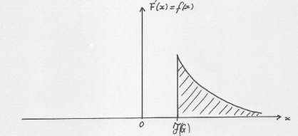
Figure 1: Density of the lead time profile $f(x)={dF(x)\over dx}$ when ${\cal F}(Q)>0$.

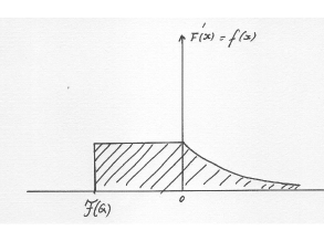
Figure 2: Density of the lead time profile $f(x)={dF(x)\over dx}$ when ${\cal F}(Q)<0.$

Remark. The alternative regimes given by Eqs.(12) and (13) can be heuristically understood by invoking the Little law which connects the average queue length $\langle Q\rangle$ with the average waiting time $\langle W\rangle$, [Cohen 73]:

$$\langle Q\rangle=\lambda\,\langle W\rangle,$$ (14)

which is independent of the scheduling policy. In view of Eqs.(11) and (14), one obviously suspects that the $LTP$ strongly depends on the sign of the difference $\langle{\cal D}\rangle-{\langle Q\rangle\over\lambda}=\langle{\cal D}\rangle-\langle W\rangle$. Intuitively, when $\langle W\rangle$ exceeds $\langle D\rangle$, it is expected, in the average, that processed jobs will be delivered too late and conversely. While the above heuristic arguments is strictly valid only for the averages, [Doytchinov et al. 2001], were able to show that in heavy traffic regimes, it also holds also for the LTP given in Eqs.(12) and (13).

Assuming that the arriving tasks have positive deadlines, the LTP as given by Eqs.(12) and (13) imply:

• a) If the left-hand support of the LTP is negative, then a job entering into service is already late, (case of Eq.(13)) see Figure 2.

• b) If the left-hand support of the LTP is positive then a jobs enters into service with a positive lead time, (case of Eq.(12)) see Figure 1. Accordingly, it is likely that the tasks will be completed before the deadline expired.

• c) The critical value $Q^{*}={\left\langle{\cal D}\right\rangle\over\lambda}$ for which ${\cal F}(Q)=0$, corresponds to a queue length for which customers are likely to become late. Choosing $Q$ exactly to $Q^{*}$, we cannot expect lateness to disappear completely but for $Q<Q^{*}$ lateness will be strongly reduced a behavior clearly confirmed by simulation experiments [Doytchinov et al. 2001] and [Baldwin et al. 2000].

• d) For deadline distributions $G(x)$ with fat tails, it follows immediately from Eqs.(12) and (13) that the LTP does possess a fat tail.

2.2.1 ”First come first served” (FCFS) scheduling policies

For the choice $g(x)=\delta(x)$, (i.e. zero deadline), the EDF scheduling policy directly coincides with the FCFS rule. Indeed, in this case ${\cal F}(Q)=0$ and the LTP density is given by Eq.(12) is a uniform probability density $U\left[-{Q\over\lambda},0\right]$, ($\left[-{Q\over\lambda},0\right]$ being its support). This expresses the fact that in the heavy traffic regime $\rho=\lambda/\mu\approx 1$, the waiting time behaves as $Q\times({1\over\mu})\approx Q\times({1\over\lambda})$ leading to a LPT linearly growing with $Q$. For general $G(x)$, the LTP associated with a FCFS scheduling rule will be given by the convolution of the deadline distribution $G(x)$ with the uniform distribution $U\left[-{Q\over\lambda},0\right]$. Indeed, adding the task deadlines with the time spent in t5he queue, we recover the tasks lead-time. Accordingly, in the heavy traffic regime and for a given queue length $Q$, one explicitly knows the LTP’s for both the EDF and the FCFS scheduling policies thus enabling to explicitly appreciate their respective characteristics. In particular, using Eqs.(12) and (13), one can conclude that for a given queue length $Q$ the FCFS scheduling rule the associated LTP $F(x)$ being the convolution of $G(x)$ with the $U\left[-{Q\over\lambda},0\right]$, it takes the form:

$$F(x)=\left\{\begin{array}[]{l@{\qquad}l}0&{\rm when}\ x<-{Q\over\lambda},\\ \\ {\lambda\over Q}\int_{-\left({Q\over\lambda}\right)}^{x}\left[G(\xi+{Q\over\lambda})\right]d\xi&{\rm when}-{Q\over\lambda}\leq x<0,\\ \\ \kappa+{\lambda\over Q}\left\{\int_{0}^{x}\left[G(\xi+{Q\over\lambda})-G(\xi)\right]d\xi\right\}&{\rm when}\ x\geq 0,\\ \end{array}\right.$$ (15)

where the constant $\kappa$ reads as:

$$\kappa={\lambda\over Q}\int_{-\left({Q\over\lambda}\right)}^{0}\left[G(\xi+{Q\over\lambda})\right]d\xi.$$

Eq.(15) allows to emphasize the following features:

• i) When the left-hand support of the deadline distribution $G(x)$ is larger than ${Q\over\lambda}$, the left boundary of the support of $F(x)$ is larger than $0$ and therefore the jobs experience no delay when entering into service.

• ii) If the left-hand support of $G(x)$ is smaller than ${Q\over\lambda}$, then it may happen that the LTP exhibits a negative left-hand support under the FCFS policy and a positive left-hand support under the EDF scheduling rule. Hence in this last situation, the FCFS policy would deliver tasks with lateness while the EDF tasks will be processed in due time. This explicitly confirms intuition that EDF is indeed an efficient policy. It has been shown that the EDF scheduling rule is optimal for minimizing the number of jobs processed after the deadline [Panwar et al. 88].

• iii) If $G(x)$ exhibits a fat tail for $x\rightarrow\infty$ so has the LTP and this whatever the scheduling rule in use. This can e directly verified from Eq.(15) by studying the LTP density $f(x)={dF(x)\over dx}$ for $x\rightarrow\infty$, we have:

  $$f(x)={\lambda\over Q}\left[G(x+{Q\over\lambda})-G(x)\right],\qquad\qquad{\rm for}\qquad x\rightarrow\infty,$$

  which when $G(x)\sim 1-x^{-q}$ and for ${Q\over\lambda}<{\rm const}$ takes the form

  $$f(x)\sim x^{-(q+1)},\qquad\qquad{\rm for}\qquad x\rightarrow\infty.$$ (16)

  Hence, the LTP inherits the fat tail property of $G(x)$ and this even when using the optimal EDF scheduling rule - a fully explicit illustration involving the Pareto probability distribution is given in the Appendix B.

The results obtained for the LTP, enable to get the asymptotic properties of the waiting time distribution WTD. Indeed, under the EDF policy, the more urgent jobs are served first and therefore the waiting time before service of the queueing jobs will be larger or equal to the lead-time. Accordingly, if the LTP exhibits a fat tail distribution so will the WTD. Hence, while the EDF policy decreases, compared with the FCFS rule, the number of jobs served after their deadline, it cannot get rid of the fat tails generated by the deadline probability distribution $G(x)$. Let us emphasize here, the fat tails of the LTP (and hence of the WTD) are here entirely due to $G(x)$ and his asymptotic behavior of the LTP is shared by both the EDF and FCFS policies. This is fundamentally different from the frozen in time PI models discussed in [Barabasi 2005], [Vázquez 2005] and [Vázquez et al. 2006] where the fat tail behavior does not depend on $G(x)$. This can be heuristically understood as, in [Barabasi 2005], [Vázquez 2005] and [Vázquez et al. 2006], the fat tail is mainly due to the low priority jobs which, as no aging mechanism occurs, are likely to never be served. Note that in [Barabasi 2005], [Vázquez 2005] and [Vázquez et al. 2006], stable queueing models, (i.e. those for which the traffic $\rho<1$), fat tails of the WTD disappear under a FCFS scheduling rule. Indeed without priority scheduling, the WTD always follows an exponential asymptotic decaying behavior. In presence of time dependent PI, all tasks do finally acquire a high priority and this aging mechanism precludes the formation of a fat tail solely due to the scheduling rule. Accordingly, in presence of aging PI, the generation of WTD with fat tails will be due to $G(x)$.

3 Conclusion and summary

There are several possibilities to analytically discuss the scheduling of tasks in QS with time dependent priority indices and to infer on the existence of fat tails for the asymptotic behavior of the resulting WTD. In this note, we propose two distinct models where an explicit analysis can be developed. Our first model is directly inspired by the study of age classes in population dynamics where the mortality rate increases with the age of the individuals. In this context, identifying the service of the QS with the death of an individual, this dynamics is closely related to the scheduling based on PI, the indices here being the age of the individuals and the immigration with different ages plays the role of incoming tasks with different priorities. For this class of dynamics, it is straightforward to show that fat tails of the WTD can develop on the onset of stability of the population model. As in the original Barabási model, the tail behavior of the WTD does not depend on the detail nature of the PI but only on the scheduling rule - (corresponding in the population model to the mortality rate). Our second modeling frame which is closer to the Barabási original idea, we consider a classic QS in which the scheduling rule is based on the deadlines attached to each incoming tasks. As time flows, the deadlines reduce and hence the waiting tasks acquire a higher priority to be processed. In the heavy traffic limit, i.e. for regimes where the law of large numbers dominate, it is possible to analytically derive the lead-time profile (lead-time = deadline minus the time elapsed in queueing) of the waiting tasks and from this to get information on the asymptotic behavior of the associated WTD. In this case and contrary to the conclusions exposed in [Barabasi 2005], [Vázquez 2005] and [Vázquez et al. 2006], the scheduling rule solely cannot generate fat tails in the WTD. Fat tail in [Barabasi 2005], [Vázquez 2005] and [Vázquez et al. 2006] are due to low priority jobs which are likely to never be served. This possibility disappears when time-dependent PI are considered as, due to aging, initially low priority tasks do acquire, with time, high priorities and hence will not stay unprocessed forever. This precludes the formation of fat tails in the WTD. We finally observe that, in this second class of models, the only possibility to generate fat tails is to feed the QS with tasks deadlines drawn from a fat tail distribution.

Acknowledgements. M.O.H. thanks numerous fruitful discussions with Olivier Gallay and Roger Filliger.

Appendix A - Waiting time distributions for QS with fat tail service times

Let us reproduce here a result recently derived in [Boxma et al. 2004]:

Theorem 1. Assume that the (random) service time in a $M/G/1$ QS is drawn from a PDF with a regularly varying tail at infinity with index $\nu\in(-1,-2)$, (regularly varying with index $\nu\in(-1,-2)$ $\Rightarrow$ fat tail with index $\nu\in(-1,-2)$). For this range of asymptotic behaviors of the PDF, the first moment $\beta$ of the service exists. Assume further that the service is delivered according to a random order discipline. Then the waiting time distribution $W_{{\rm ROS}}$ exhibits a fat tail with index $\left(1-\nu\right)\in(-1,0)$ and more precisely, we can write:

$${\rm Prob}(W_{{\rm ROS}}>x)\varpropto C{\rho\over 1-\rho}\,{h(\rho,\nu)\over\beta\,\Gamma(2-\nu)}\,x^{1-\nu}\,{\cal L}(x),$$ (17)

where $\rho<1$ is the traffic intensity, $\beta$ the average service time, ${\cal L}(x)$ a slowly varying function and

$$h(\rho,\nu):=\int_{0}^{1}f(u,\rho,\nu)du,$$

with:

$$f(u,\rho,\nu):={\rho\over 1-\rho}\left({\rho\,u\over 1-\rho}\right)^{\nu-1}\,\left(1-u\right)^{{1\over 1-\rho}}+\left(1+{\rho\,u\over 1-\rho}\right)^{\nu}\,\left(1-u\right)^{{1\over 1-\rho}-1}.$$

The fat tail behavior given in Eq.(17) is therefore entirely inherited from the fat tail behavior of the service and is not affected by any reduction of the trafic intensity $\rho$. Note also that change of the scheduling rule cannot get rid of this fat tail behavior. This point can be explicitly observed in [Cohen 1973], [Pakes 1975] who show that for the previous $M/G/1$ QS with a random order service (ROS) service discipline, one obtains:

$${\rm Prob}(W_{{\rm ROS}}>x)\varpropto h(\rho,\nu){\rm Prob}(W_{{\rm FCFS}}>x),\,\,\,\,\,\,\,\,\,\,\,{\rm for}\,\,\,x\rightarrow\infty,$$ (18)

from which we directly observe that the fat tail in the asymptotic behavior in not altered by a change of the scheduling rule.

Note finally that for the $M/M/1$ QS, (i.e. exponential service distributions and hence no fat tail), [Flatto 1997] shows that the random order service scheduling rule yields:

$${\rm Prob}(W_{{\rm ROS}}>x)\varpropto C_{\rho}x^{-{5\over 6}}\,e^{-\gamma x-\delta x^{{1\over 3}}},\,\,\,\,\,\,\,\,\,\,\,{\rm for}\,\,\,x\rightarrow\infty,$$ (19)

with

$$C(\rho)=2^{2\over 3}3^{-{1\over 2}}\pi^{{5\over 6}}\rho^{{17\over 12}}{1+\rho^{{1\over 2}}\over\left[1-\rho^{{1\over 2}}\right]^{3}}\exp\left\{{1+\rho^{{1\over 2}}\over 1-\rho^{{1\over 2}}}\right\},$$

$$\gamma=\left(\rho^{-{1\over 2}}-1\right)^{2}\,\,\,\,\,\,\,\,\,\,\,{\rm and}\,\,\,\,\,\,\,\,\,\,\delta=3\left[{\pi\over 2}\right]^{{2\over 3}}\rho^{-{1\over 6}},$$

which has to be compared with the FCFS scheduling discipline, which for the same $M/M/1$ QS reads as, [Cohen 1973]:

$${\rm Prob}(W_{{\rm FCFS}}>x)={1\over\beta}(1-\rho)e^{-{1\over\beta}(1-\rho)x}.$$ (20)

While the detailed behaviors given by Eq.(19) and (20)clearly differ, they however both share, in accord with [Barabási 2005], an exponential decay.

Appendix B - Deadline drawn from Pareto distribution

Here, we focus on:

$$G(x)=\left\{\begin{array}[]{l@{\qquad}l}0&{\rm when}\ {x\over B}<1,\\ \\ 1-\left({B\over x}\right)^{(\omega-1)}&{\rm when}\ {x\over B}\geq 1,\qquad\omega>1,\\ \end{array}\right.$$ (21)

which has no moment of order $\omega-1$ or higher. For $\omega>2$, we have $\left\langle{\cal D}\right\rangle=\left[{\omega-1\over\omega-2}\right]\,B$:

$${\cal F}(Q)=\left\{\begin{array}[]{l@{\qquad}l}B\left({B\lambda\over Q(\omega-2)}\right)^{\left({1\over\omega-2}\right)}&{\rm when}\ {Q\over\lambda}\leq{B\over\omega-2},\\ \\ \left({\omega-1\over\omega-2}\right)B-{Q\over\lambda}&{\rm when}\ {Q\over\lambda}>{B\over\omega-2}.\\ \end{array}\right.$$ (22)

Using Eqs.(12) and (13), the LTP distribution reads as:

$${Q\over\lambda}\geq{B\over\omega-2}\quad\Rightarrow\quad F(x)=\left\{\begin{array}[]{l@{\qquad}l}0,&{\rm when}\ x\leq{\cal F}(Q),\\ \\ 1-{\lambda\over Q}\left({\omega-1\over\omega-2}B-x\right),&{\rm when}\ {\cal F}(Q)\leq x<B,\\ \\ 1-{B\lambda\over Q(\omega-2)}\left({B\over x}\right)^{\omega-2}.&{\rm when}\ x\geq B.\end{array}\right.$$ (23)

$${Q\over\lambda}<{B\over\omega-2}\quad\Rightarrow\quad F(x)=\left\{\begin{array}[]{l@{\qquad}l}0,&{\rm when}\ x\leq{\cal F}(Q),\\ \\ 1-{B\lambda\over Q(\omega-2)}\left(B\over x\right)^{\omega-2}.&{\rm when}\ x>{\cal F}(Q).\\ \end{array}\right.$$ (24)

Eqs.(23) and (24) exhibit a fat tail with power $\omega-2$. Note that, Eq.(24), implies that for ${\omega>2}$ and for ${Q\over\lambda}<{B\over(\omega-2)}$, the EDF scheduling policy part of the tasks enter into the service before the due date expired. Finally note also, that for $\omega\leq 2$, no moments exists for the deadline distribution and hence the theory [Doytchinov et al. 2001] cannot be applied directly. We conjecture that for these regimes no scheduling rule will be able to deliver tasks in due time.

References

[Baldwin et al. 2000] R.O. Baldwin, N. J. Davis, J. E. Kobza and S. F. Mikdiff. Real-time queueing theory : A tutorial presentation with an admission control application. Queueing Syst. Th. and Appl.35(1-4), (2000), 1-21.

[Barabási 2005] A.-L. Barabási. The origin of bursts and heavy tails in human dynamics. Nature 435, (2005), 207.

[Blanchard et al. 2004] Ph. Blanchard and M.-O. Hongler. Self-organization of critical behavior in controlled general queueing systems. Phys. Lett. A 323(1-2), (2004), 63-66.

[Boxma et al. 2004] O.J. Boxma, S.G. Foss, J.M. Lasgouttes and R. Nùñez Queija. Waiting time asymptotic in the single server queue with service in random order, Queueing Systems 46, (2004), 35-73.

[Brauer et al. 2001]. F. Brauer and C. Castillo-Chávez. Mathematical Models in Population Biology and Epidemiology. Text in Applied Mathematics 40, Springer (2001).

[Cohen 1973] J. Cohen. Some results on regular variation for distributions in queueing and fluctuation theory. J. Appl. Probab. 10, (1973), 343-353.

[Doytchinov et al. 2001] B. Doytchinov, J. Lehozcky, S. Shreve. Real-time queues in heavy traffic with earliest-deadline-first queue discipline. Ann. Appl. Probab. 11, (2001), 332-378.

[Dusonchet et al. 2003] F. Dusonchet and M.-O. Hongler. Continuous-time restless bandit and dynamic scheduling for make-to-stock production. IEEE Trans Robot and Autom. 19(6), (2003) 997-990.

[Filliger et al. 2005] R. Filliger and M.-O. Hongler. Syphon dynamics - A soluble model of multi-agents cooperative behavior. Europhys. Lett. 70(3), (2005), 285-291.

[Flatto 1977] L. Flatto. The waiting time distribution for the random order service $M/M/1$ queue. The Annals of Probab. 7, (2), (1997) 382-409.

[Lehozcky 1996] J. Lehozcky Real-time queueing theory. In Proceed. of the IEEE Real-time system symposium, New-York (1996), 186-195.

[Lehozcky 1997] J. Lehozcky Using real time queueing theory to control lateness in realtime systems. Perfom. Eval. 25 (1997), 158-168.

[Pakes 1975] A. G. Pakes. On the tails of waiting-time distributions. J. Appl. Prob . 12, (1975), 555-564.

[Panwar et al. 88] S. Panwar and D. Townsley and J.K Wolf Optimal Scheduling Policies for a Class of Queues with Customers Deadlines for the Beginning of services. J. of the ACM 35,(4), (1988), 832-844.

[Vázquez 2005] A. Vázquez. Exact Results for the Barabási Model of Human Dynamics. Physical Review Letters 95, (2005), 248701.

[Vázquez et al 2006] A. Vázquez, J. G. Oliveira, Z. Dezsö, K.-I. Goh, Kondor I. and A.-L. Barabási. Modeling Bursts and Heavy Tails in Human Dynamics, Phys. Rev. E 73(3), (2006), 036127.