Effective Hamiltonians for some highly frustrated magnets

Abstract

In prior work, the authors developed a method of degenerate perturbation theory about the Ising limit to derive an effective Hamiltonian describing quantum fluctuations in a half-polarized magnetization plateau on the pyrochlore lattice. Here, we extend this formulation to an arbitrary lattice of corner sharing simplexes of $q$ sites, at a fraction $(q-2k)/q$ of the saturation magnetization, with $0<k<q$. We present explicit effective Hamiltonians for the examples of the checkerboard, kagome, and pyrochlore lattices. The consequent ground states in these cases for $k=1$ are also discussed.

1 Introduction

Despite decades of theoretical and experimental work, frustrated quantum magnets continue to be an exciting subject for current research both experimentally and theoretically. Analytic approaches to such spin systems have, however, not often directly confronted experiment. Theoretically, the semi-classical spin-wave theory (i.e $1/s$ expansion) has probably been most successful. For instance, quantum corrections to the classical staggered magnetization are known to be small even for $s=1/2$ in the unfrustrated square lattice. The utility of the $1/s$ expansion, however, diminishes rapidly as frustration is increased.

This situation is at its extreme in the class of maximally geometrically frustrated structures, which includes the two-dimensional kagome and checkerboard lattices, and the three-dimensional pyrochlore lattice. These structures have the common feature that they can be decomposed into distinct “corner sharing” simplexes, clusters of spins in which all pairs are connected by nearest neighbor bonds, such that the entire lattice is covered by these simplexes, and different simplexes share at most one site and no bonds. The nearest-neighbor antiferromagnet on this lattice has the property that its Hamiltonian can be written entirely in terms of the sum of spins on each simplex. At the classical level, this implies a large degeneracy, since any change in configuration which keeps this sum constant on each simplex cannot change the energy. This leads to considerable technical difficulties in the $1/s$ expansion, which have been addressed in tour-de-force work by Henley and collaborators [1]. An unfortunate outcome of this work is that the leading order ($O(1/s^{0})$) corrections (spin-wave zero point energy) do not fully split the classical degeneracy in most interesting cases. Given the challenges already present at $O(1/s^{0})$, it is not surprising that higher order corrections in $1/s$, which would be necessary to resolve the degeneracy fully and determine the quantum ground state for large $s$, are so far not available.

In recent work, we have demonstrated that the resolution of the classical degeneracy can be understood in an alternate approach, based on perturbation theory about the limit of strong Ising exchange anisotropy. That is, we consider the XXZ model

$${\mathcal{H}}=J\sum_{\langle ij\rangle}S^{z}_{i}S^{z}_{j}+\frac{J}{2}\alpha\sum_{\langle ij\rangle}\left(S_{i}^{+}S_{j}^{-}+h.c.\right)-H\sum_{j}S^{z}_{j}\;,$$ (1)

and carry out perturbation theory in $\alpha$ for the degenerate ground state manifold. This is expected to be a reasonable approximation in many problems of interest. First, the semiclassical approach demonstrates rather generally that in these models quantum fluctuations favor collinear ordered states, in which all spin expectation values are aligned along a particular, e.g. $S^{z}$ axis. Choosing Ising anisotropy only selects this axis, but does not prejudice the ordering beyond this choice. Second, some of the most interesting applications are to magnetization plateaus, which often appear in frustrated magnets (e.g in pyrochlores [4]). General arguments (see e.g. [2]) imply that ordering is again collinear on such plateaus. Moreover, since such a plateau occurs in a substantial applied field, the component of each spin parallel to this field is clearly on average larger than its transverse ones. Furthermore, the introduction of Ising anisotropy does not modify the symmetry of the Hamiltonian in this case. In [3], we have demonstrated explicitly how to carry out easy-axis degenerate perturbation theory for a magnetization plateau on the pyrochlore lattice at half the saturation polarization. The result was an effective quantum “dimer” Hamiltonian describing the splitting of the degenerate manifold of plateau states.

In this paper, we describe the generalization of these results to the lattices described above, for various zero field and plateau states. Our results are obtained under the assumption that each corner-sharing simplex contains $q$ sites, and that the Ising ground state manifold is comprised of states with $k$ “minority” ($S^{z}=-s$) and $q-k$ “majority” ($S^{z}=+s$) spins per simplex. The cases mentioned above correspond to $q=3,k=1$ (kagome lattice at magnetization $M=1/3M_{s}$), $q=4,k=2$ (checkerboard and pyrochlore lattices at $M=0$), $q=4,k=1$ (checkerboard and pyrochlore lattices at $M=1/2M_{s}$). For the $k=1$ cases, the corresponding effective Hamiltonians are generalized “quantum dimer models”, and we discuss their ground states based on known results and simple arguments. The solution for the ground states of the $k=2$ models (corresponding to zero magnetization) on the pyrochlore and checkerboard lattices are left for future work.

The remainder of the paper is organized as follows. In section 2, we describe the derivation of the effective Hamiltonians. In section 3, we give explicit forms for the above-mentioned lattices. In section 4 we discuss the ground states of the effective models in the $k=1$ cases.

2 Resume of Method

In this section, we review the degenerate perturbation theory (DPT) methods developed in [3]. Because the fine details are given already in [3], we will highlight only the main points and those modifications needed for the more general applications in this paper.

For any (apart from a set of measure zero) fixed field $H$ in the Ising limit $\alpha=0$, the ground states of equation 1 comprise a massively degenerate manifold of configurations of constant magnetization – “plateau states”. Specifically, in these configurations (as indicated in the introduction) all spins are aligned along the field axis, i.e $S_{i}^{z}=s\sigma_{i}$, with $\sigma_{i}=\pm 1$, and every simplex contains $k$ minority ($\sigma_{i}=-1$) spins and $q-k$ majority ($\sigma_{i}=+1$) spins. We seek an effective Hamiltonian in this degenerate subspace.

We follow the Brillouin-Wigner formulation of DPT. The ground state wavefunction satisfies the exact equation

$$\left[E_{0}+{\mathcal{P}}{\mathcal{H}}_{1}\sum_{n=0}^{\infty}{\mathcal{G}}^{n}{\mathcal{P}}\right]|\Psi_{0}\rangle=E|\Psi_{0}\rangle={\mathcal{H}}_{\textrm{eff}}|\Psi_{0}\rangle,$$ (2)

where the operator ${\mathcal{G}}=\frac{1}{E-{\mathcal{H}}_{0}}\left(1-{\mathcal{P}}\right){\mathcal{H}}_{1}$. Here ${\mathcal{H}}_{0}=\left.{\mathcal{H}}\right|_{\alpha=0}$, and ${\mathcal{H}}_{1}={\mathcal{H}}-{\mathcal{H}}_{0}$. Because the resolvent contains the exact energy $E$, equation (2) is actually a non-linear eigenvalue problem. However, to any given order of DPT, $E$ may be expanded in a series in $\alpha$ to obtain an equation with a true Hamiltonian form within the degenerate manifold. Each factor of ${\mathcal{G}}$ is at least of $O(\alpha)$ due to the explicit factor in ${\mathcal{H}}_{1}$, with higher order corrections coming from the expansion of $E$. Following the strategy of [3], we will obtain the lowest order non-constant diagonal and off-diagonal terms in ${\mathcal{H}}_{\textrm{eff}}$. Because we seek only the lowest order term of each type, it is admissible to replace $E$ by $E_{0}$ in ${\mathcal{G}}$, a considerable simplification.

With this replacement, we need only calculate the successive applications of ${\mathcal{G}}$ and ${\mathcal{H}}_{1}$ in equation 2 starting from some arbitary initial state. This is facilitated by the simple geometry of the lattice, and by symmetry. The Hamiltonian in equation 1 has a global $U(1)$ symmetry, corresponding to rotations about the z-axis. As such, the z-component of the total magnetization $\sum_{j}S^{z}_{j}$ is a conserved quantity at every stage of DPT. This leads to some important properties of the resolvent operator ${\mathcal{R}}=({\mathcal{H}}_{0}-E_{0})^{-1}$:

$${\mathcal{R}}^{-1}=\frac{J}{2}\sum_{ij}\Gamma_{ij}S_{i}^{z}S_{j}^{z}-H\sum_{j}S_{j}^{z}-E_{0}\;,$$ (3)

where $\Gamma_{ij}$ is the adjacency matrix, i.e. $\Gamma_{ij}=1$ if $i,j$ are nearest-neighbors and $\Gamma_{ij}=0$ otherwise. We will need the action of ${\mathcal{R}}$ not on states in the ground state manifold, but on an arbitrary virtual state reached in a DPT process. We describe these states by integers $m_{j}$, with $0\leq m_{j}\leq 2s$, such that $S_{j}^{z}=\sigma_{j}(s-m_{j})$. Conservation of magnetization enforces $\sum_{j}m_{j}\sigma_{j}=0$ for all virtual states. One may readily confirm the additional identity

$$\sum_{i}\Gamma_{ij}\sigma_{i}=2(q-2k)-2\sigma_{j},$$ (4)

which results from the constraints on the spin configurations contained on the two simplexes sharing site $j$. Using these two relations, the inverse resolvent can be rewritten as

$${\mathcal{R}}^{-1}=\frac{J}{2}\sum_{ij}\Gamma_{ij}m_{i}m_{j}\sigma_{i}\sigma_{j}+2sJ\sum_{j}m_{j}\;.$$ (5)

Note that the resolvent only involves variables on the sites that are modified in the DPT process, since all other $m_{j}=0$. With this observation, we are ready to describe the calculations.

We first consider the off-diagonal term, which must cause transitions from one plateau state to another. To maintain the constraint requires flipping spins $\pm s\rightarrow\mp s$ in a closed loop of alternating $\pm s$ spins. This is because an open string of spin transfer changes the number of minority sites on the simplexes at the two ends of the string: one suffers a deficit, and the other suffers a surplus. Since ${\mathcal{H}}_{1}$ is a sum of spin transfer operators on links of the lattice, one may readily deduce the order at which the first off-diagonal term appears, without calculating it explicitly. The smallest even-length non-trivial loop in the lattice (non-retracing walk residing on more than one simplex) is of some even length $L$ ($L=6$ for pyrochlore and kagome, $L=4$ for Checkerboard) and surrounds a plaquette of the lattice. This loop contains $L/2$ minority sites that will be converted to majority sites. Each flipping takes $2s$ operations of ${\mathcal{H}}_{1}$, so that the off-diagonal term is of order $\alpha^{sL}$. For large $s$, this becomes of very high order and entirely negligible. It can however be important for moderate values of $s$.

As is clear from this discussion, the lowest-order off-diagonal term generates a single process: flipping all spins along one length-$L$ loop. Thus it has the general form

$${\mathcal{H}}_{\textrm{off diagonal}}=-K_{L}(s)\alpha^{Ls}J\sum_{\mathcal{P}}\left(|\downarrow\uparrow\ldots\downarrow\uparrow\rangle\langle\uparrow\downarrow\ldots\uparrow\downarrow|+h.c.\right)\;.$$ (6)

What remains to be calculated is the coefficient $K_{L}(s)$ multiplying the plaquette flipping operator. In [3], an iterative method was developed to calculate this amplitude by considering successive applications of ${\mathcal{H}}_{1}$ on any initial state. Because all the spin-flips occurring in any given process are on a single length-$L$ loop, the calculation is insensitive to the global structure of the lattice, and depends only upon the length of the plaquette. This implies that, for hexagonal plaquettes, the off-diagonal coeffcient is identical to that calculated in [3], even on the kagome lattice! The values for $K_{6}(s)$ for $s=1/2,1,3/2,2,5/2$ were calculated in [3].

For the square plaquette lattices, the calculation is actually significantly simpler. At a given stage in the DPT process, the resolvent can be calculated using the number of times every (alternating) link has undergone spin transfer up to that step. For the square plaquette, there are only two such links, as opposed to three for the hexagonal plaquette. After $\ell$ link operations, one finds that the resolvent is given simply by

$${\mathcal{R}}_{\ell}^{-1}=J\ell(4s-\ell).$$ (7)

Applying this formula, the off-diagonal coefficient is determined explicitly for any value of $s$:

$$K_{4}(s)=\frac{4s}{2^{4s}}\frac{[(2s)!]^{2}}{(4s-1)!}.$$ (8)

We now turn to the diagonal terms in DPT. Unlike the off-diagonal terms above, these occur at a fixed order in $\alpha$ independent of $s$. To understand at what order this occurs, first note that a diagonal DPT process of order $n$, which starts out from some plateau state, and returns to it in the end can have at most $n$ sites modified, since each site that is modified must be modified again at least once in order to return to its original configuration. From the structure of the resolvent discussed above, we say that at $n^{\rm th}$ order, the diagonal effective Hamiltonian is a sum of terms, each of which involves at most $n$ Ising spin variables. The diagonal effective Hamiltonian therefore has the general structure

$${\mathcal{H}}_{\rm eff}[\{\sigma_{i}\}]=\sum_{n}\sum_{G_{n}}\sum_{a_{1}\ldots a_{n}}\!\!\!\left(\prod_{(ij)\in G_{n}}\Gamma_{a_{i}a_{j}}\right)f_{G_{n}}(\sigma_{a_{1}},\ldots,\sigma_{a_{n}}),$$ (9)

where $G_{n}$ denotes a “graph” of lines connecting the labels $a_{1}\ldots a_{n}$ visualized as points, i.e. a set of unordered pairs of these labels. Note that the dependence upon the lattice geometry enters only through $\Gamma_{ij}$. This function can be derived from direct evaluation of equation 2 using the simplified resolvent, as outlined in [3].

Remarkably, for any lattice composed of corner-sharing simplexes, all terms in equation 9 with $n<L$ are constants in the ground-state manifold. This was demonstrated in [3] for the case of the pyrochlore lattice (where $L=6$), but the arguments follow more generally. We outline the basic ideas, referring to [3] for details. First, one can show that all “contractible” diagrams, in which at least one point in $G_{n}$ is connected to less than 2 other points, can be reduced to a term of lower order. This follows by explicitly summing over the corresponding index (e.g. $a_{n}$), using the identity in equation 4 and the constant total magnetization. Second, one shows that “non-contractible” diagrams with $n<L$ are constant by a different argument. First, one notes that the sites $a_{i}$ for which $\prod_{(ij)\in G_{n}}\Gamma_{a_{i}a_{j}}\neq 0$ must form a compact cluster, and for $n<L$ this cluster cannot span the smallest non-trivial loop. Summing over all clusters satisfying $\prod_{(ij)\in G_{n}}\Gamma_{a_{i}a_{j}}\neq 0$, one again obtains constant. This is essentially because any permutation of the cluster sites $a_{i}$ gives another cluster, and the sum over all such permutations can be reduced using the fact that the allowed spin configurations of a simplex are all permutations of one reference configuration (with $k$ minority spins on $q$ sites).

The lowest non-constant term in the diagonal effective Hamiltonian therefore comes at order $n=L$. Indeed, by application of the same arguments described above, only one distinct term at this order is non-constant: the one for which $G_{n}$ consists of a single loop connecting all labels, i.e. $\prod_{(ij)\in G_{L}}\Gamma_{a_{i}a_{j}}=\Gamma_{a_{1}a_{2}}\Gamma_{a_{2}a_{3}}\cdots\Gamma_{a_{L-1}a_{L}}\Gamma_{a_{L}a_{1}}$. This term can be explicitly evaluated, and has non-constant contributions only when $(a_{1},\cdots,a_{L})$ lie sequentially along one of the length $L$ loops of the physical lattice. Evaluating $f_{G_{n}}$ at the spins of these sites leads to the final expression for the diagonal energy function.

3 Results

The diagonal effective Hamiltonian obtained above can in all cases be written as a sum over plaquettes

$${\mathcal{H}}_{\textrm{diag}}=\sum_{\mathcal{P}}{\mathcal{E}}_{\mathcal{P}}(\sigma_{{\mathcal{P}}1},\cdots,\sigma_{{\mathcal{P}}L})\;,$$ (10)

where $\sigma_{{\mathcal{P}}1}\cdots\sigma_{{\mathcal{P}}L}$ are the $L$ sites ordered sequentially around the plaquette ${\mathcal{P}}$. We choose the function ${\mathcal{E}}$ to have cyclic symmetry. For the kagome and pyrochlore lattices, the plaquettes are hexagonal, bounded by 6 links. For the Checkerboard lattice, the plaquettes are square, bounded by 4 links.

Remarkably, the manipulations in the previous section imply that, as a function ${\mathcal{E}}_{\mathcal{P}}(\sigma_{1},\cdots,\sigma_{L})$ is the same for all lattices with the same plaquette size (4,6,8 etc.), for any $k$. The differences arise in the allowed plaquette configurations, which depend strongly on $q$ and $k$. This function is most conveniently described by giving the energies for all possible plaquette configurations. For the lattices with hexagonal plaquettes we find

$${\mathcal{E}}_{0}= {\mathcal{E}}_{\bar{0}}=0,\hskip 144.54pt{\mathcal{E}}_{1}={\mathcal{E}}_{\bar{1}}=\frac{1}{4}{\mathcal{E}}_{2}=\frac{1}{4}{\mathcal{E}}_{\bar{2}}=-\frac{Js^{3}\alpha^{6}}{32(1-4s)^{2}},$$ (11)

$${\mathcal{E}}_{3}= {\mathcal{E}}_{\bar{3}}=-\frac{Js^{4}\left(512s^{2}-256s+33\right)\alpha^{6}}{16(3-8s)^{2}(4s-1)^{3}},\hskip 57.81621pt{\mathcal{E}}_{4}={\mathcal{E}}_{\bar{4}}=-\frac{J(1-8s)^{2}s^{4}\alpha^{6}}{8(4s-1)^{5}},$$

$${\mathcal{E}}_{5}= -\frac{6Js^{5}\left(3072s^{5}-4352s^{4}+2432s^{3}-660s^{2}+88s-5\right)\alpha^{6}}{(3-8s)^{2}(4s-1)^{5}\left(24s^{2}-22s+5\right)},\hskip 36.135pt{\mathcal{E}}_{6}=6{\mathcal{E}}_{\bar{1}},$$

$${\mathcal{E}}_{7}= -\frac{Js^{4}\left(128s^{2}-40s+3\right)\alpha^{6}}{8(1-4s)^{4}(8s-3)}-\frac{4Js^{6}\left(5184s^{3}-3600s^{2}+789s-56\right)\alpha^{6}}{3(4s-1)^{5}\left(64s^{2}-32s+3\right)^{2}\left(72s^{2}-18s+1\right)}$$

$$- \frac{Js^{4}\alpha^{6}}{2(1-4s)^{2}(8s-3)}\;.$$

The various plaquettes types are shown in figure 1(a). For the pyrochlore $k=2$ plateau, all 13 plaquette configurations in figure 1(a) are possible. Not surprisingly, the energies for plaquette configurations with up and down spins swapped are identical, since in this case ($k=2,q=4$) there are equal numbers of minority and majority sites on each simplex. Interestingly, this case can be interpreted as an “ice model”, in which the two down spins on a tetrahedron indicate the locations of protons on the oxygen atom at its center.

(a) hexagonal plaquette

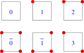
(b) square plaquette

Figure 1: (Color online) Hexagonal and square plaquette Ising configurations. The minority sites are denoted by solid (red) circles.

For the kagome $k=1$ antiferromagnet at $1/3$ magnetization and the pyrochlore $k=1$ antiferromagnet at $1/2$ magnetization (the subject of [3]), there are only 5 allowed plaquette configurations, those with no two neighboring minority sites. These are the plaquettes configurations labeled $0,1,3,4,5$. Their energies are the same expressions as in 11.

For lattices with square plaquettes, we find

$${\mathcal{E}}_{0}= {\mathcal{E}}_{\bar{0}}=0,\hskip 137.31255pt{\mathcal{E}}_{1}={\mathcal{E}}_{\bar{1}}=-\frac{Js^{3}\alpha^{4}}{2(4s-1)^{2}},$$ (12)

$${\mathcal{E}}_{2}= -\frac{Js^{3}\left(64s^{2}-24s+3\right)\alpha^{4}}{2(4s-1)^{3}(8s-1)},\hskip 36.135pt{\mathcal{E}}_{3}=-\frac{8Js^{4}\left(8s^{2}-5s+1\right)\alpha^{4}}{(4s-1)^{3}\left(16s^{2}-14s+3\right)}\;.$$

The square plaquettes types are described in figure 1(b). The $k=2$ (zero magnetization) plateau of the checkerboard lattice allows all 6 plaquette types outlined in figure 1(b). For $k=1$ ($1/2$ magnetization), only types $0,1,3$ are allowed.

As explained in detail in [3], these energies are actually slightly redundant. To see this, first define $x_{a}$ as the fraction of plaquettes in the lattice in configuration $a$. Then the energy per plaquette of any state is given by

$${\mathcal{H}}_{\textrm{diag}}/N=\sum_{a}x_{a}{\mathcal{E}}_{a},$$ (13)

where $N$ is the total number of plaquettes. Now one notices that the fractions obey two global constraints: first the fractions must sum to $\sum_{a}x_{a}=1$, and second, the total fraction of minority sites must be $\frac{k}{q}$. Denoting the fraction of minority sites in each plaquette configuration by $M_{a}$, the latter constraint implies $\sum_{a}x_{a}M_{a}=\frac{k}{q}$. Because of these two constraints, we see that it is possible to shift the energies in equation 13 in such a way as to change the energy per plaquette by a constant for all allowed configurations: ${\mathcal{E}}_{a}\rightarrow c_{0}+c_{1}M_{a}$, with $c_{0}$ and $c_{1}$ arbitrary. By appropriate choice of these constants, one can tune two plaquette configuration energies to zero.

4 Lowest energy states for the $k=1$ effective Hamiltonians

The plateau states described above can always be mapped to (sometimes overlapping) dimer coverings on lattices with sites at the center of each simplex, and links passing through every site. Each site in the dimer lattice therefore has $q$ links emanating from it. A minority site in the original lattice corresponds to the presence of a dimer on the corresponding link in the dimer lattice. With $k$ minority sites, each site in the dimer lattice is covered by $k$ dimers. The diagonal term in each effective Hamiltonian simply assigns different energies to the various dimer coverings. For the cases with $k=1$, which correspond to plateau states with non-vanishing magnetization, these models are of the form of generalized Quantum Dimer Models (QDMS)[5], though often with a modified and more complicated diagonal term. In this section, we use known results for these QDMs and simple optimization arguments to analyze the particular examples for which we have derived the effective Hamiltonian in the previous section.

4.1 Checkerboard lattice

First we address the simplest effective Hamiltonian – the one obtained for the checkerboard lattice. The dimer lattice is the square lattice, and so for $k=1$ the Hilbert space of dimer coverings is the same one of [5].

For $k=1$, there are only three plaquette configurations possible, so we shift energies so that only the energy of the flippable plaquette (type 3) is non-zero and equal to $V={\mathcal{E}}_{0}+{\mathcal{E}}_{3}-2{\mathcal{E}}_{1}$. For $s>\frac{1}{2}$ it is straightforward to show that $V<0$. For $s=\frac{1}{2}$ there is a divergence, which indicates that the procedure is invalid in that case. For spin-$1/2$, this occurs because the off-diagonal term appears already at order $\alpha^{2}$, whereas the diagonal term appears at order $\alpha^{4}$. Because off-diagonal processes are possible already at second order, some of the intermediate projection operators in equation 2 must be treated more carefully in that case. However, for $s=\frac{1}{2}$ the off-diagonal term is in any case dominant, so the diagonal term can be neglected. Therefore we take $V=0$ in this case, and for all $s\geq\frac{1}{2}$, we have $V\leq 0$.

Adding the lowest order off-diagonal term, which flips between the two type 3 plaquette configurations on a given plaquette, we find the lowest order diagonal and off-diagonal terms form a QDM of exactly the same form of [5]

$${\mathcal{H}}_{\textrm{QDM}}=V\sum_{\mathcal{P}}\left({\centering\includegraphics[width=101.17755pt]{Square_QDM.eps}\@add@centering}\right)-t\sum_{\mathcal{P}}\left({\centering\includegraphics[width=101.17755pt]{Square_QDM2.eps}\@add@centering}\right)\;,$$ (14)

where $t=K_{4}(s)\alpha^{4s}J>0$.

The model 14 has undergone in-depth numerical scrutiny (see [7]), which shows that for $V/t<+0.6\pm 0.05$ one obtains a columnar phase, in which the dimers preferentially sit on staggered columns of parallel bonds. For any value of $s$, we have $V/t\leq 0$. Therefore, the ground state is always in the columnar phase.

4.1.1 Kagome lattice

Next we turn to the kagome $k=1$ plateau, in which the magnetization is $\frac{1}{3}$ of the full polarization possible. The dimer lattice in this case is the honeycomb lattice, and so for $k=1$ the Hilbert space of dimer coverings is that of the QDM of [8]. The effective Hamiltonian takes on the form

$${\mathcal{H}}_{\textrm{QDM}}=\sum_{\mathcal{P}}{\mathcal{E}}_{\mathcal{P}}-t\sum_{\mathcal{P}}\left({\centering\includegraphics[width=101.17755pt]{honeycomb_QDM.eps}\@add@centering}\right)\;,$$ (15)

with the plaquette energies defined in equation 11, and $t=K_{6}(s)\alpha^{6s}J>0$. As before, for spin $s=\frac{1}{2}$ the diagonal energies are taken to be $0$. In that case, the model reduces to a particular case of the model considered in [8], in which they find the phase is a “plaquette valence bond solid”, in which resonating plaquettes (superpositions of the two type 5 configurations) form a $\sqrt{3}\times\sqrt{3}$ sublattice of all plaqettes.

We can tune the honeycomb lattice plaquette energies so that types $0$ and $3$ have energy $0$. The remaining plaquette energies are $V_{5}=\frac{1}{2}\left(\mathcal{E}_{0}+2\mathcal{E}_{5}-3\mathcal{E}_{3}\right)$, $V_{1}=\frac{1}{2}\left(-\mathcal{E}_{0}+2\mathcal{E}_{1}-\mathcal{E}_{3}\right)$, $V_{4}=\mathcal{E}_{4}-\mathcal{E}_{3}$. From equation 11, we find that for $s\geq 1$, $V_{5}<0$ and $V_{1,4}>0$, so that the flippable plaquettes (type 5 in figure 1(a)) are favored energetically.

Ignoring the off-diagonal term for a moment, the lowest energy dimer covering configuration for the entire range of $s$ has the $\sqrt{3}\times\sqrt{3}$ structure of the columnar state of [8]. This dimer covering includes only type $0$ and type $5$ plaquettes, with $\frac{1}{3}$ of the plaquettes in the type $0$ configuration, and the remaining $\frac{2}{3}$ plaquettes in the type $5$ configuration. From the constraint on the total fraction of the minority sites $\sum_{a}x_{a}M_{a}=\frac{1}{3}$ we can immediately deduce that $x_{5}M_{5}\leq\frac{1}{3}$ since all $x_{a}\geq 0$ and all $M_{a}\geq 0$. With $M_{5}=\frac{1}{2}$ we find that $x_{5}\leq\frac{2}{3}$, so that $\sqrt{3}\times\sqrt{3}$ state has the maximum fraction of type $5$ (flippable) plaquettes we can pack on the lattice, already an indication that this is a very good energy state. Since the remaining plaquettes are of type $0$ with energy $0$, which is the second best energy possible for any plaquette configuration, this is clearly the lowest energy possible for any dimer covering in this model.

Next we will try to analyze the model 15 with the off-diagonal included. Since the diagonal term favors flippable plaquettes, it is not unreasonable to approximate $V_{1,4}\approx 0$. Then our model becomes the same as the QDM of [8]

$${\mathcal{H}}_{\textrm{QDM}}=V\sum_{\mathcal{P}}\left({\centering\includegraphics[width=101.17755pt]{honeycomb_QDM2.eps}\@add@centering}\right)-t\sum_{\mathcal{P}}\left({\centering\includegraphics[width=101.17755pt]{honeycomb_QDM.eps}\@add@centering}\right)\;,$$ (16)

where $V=V_{5}\leq 0$. Calculating the off-diagonal coefficient $t$ by the methods of section 2, we obtain $\alpha^{6(s-1)}V/t=-0.246927,-2.24511,-45.155,-1228.23$ respectively for $s=1,3/2,2,5/2$. For all $s>1$, even when extrapolating $\alpha\rightarrow 1$, we find that the ratio $V/t$ takes on a value that puts it in a columnar valence bond solid phase, according to the results of [8]. For $s=1$, the diagonal and off-diagonal terms are of the same order in $\alpha$, and the ratio $V/t\approx-0.247$ is $\alpha$-independent. However, this puts the system described by equation 16 within the quoted error bar for the transition point between the plaquette and columnar valence bond solid phases in [8]: $V/t=-0.2\pm 0.05$. The $s=1$ case may therefore be more sensitive to the values of $V_{2,4}$ than other values of $s$.

4.2 Pyrochlore lattice

Finally we turn to the case of the pyrochlore lattice. The $k=1$ case was discussed in [3], but we will give a brief summary here. As discussed in section 3, the plaquette energies are off-diagonal term are identical to those on the simpler kagome lattice. Thus the effective Hamiltonian is the same as the one given in equation 15, but with dimers on links of the diamond lattice. For sufficiently large $s$, the off-diagonal term can be neglected, and one need only find the classical dimer covering minimizing the diagonal energy. For large $s\gg 1$, this classical optimization problem could be analytically solved. The resulting “trigonal₇” state has trigonal symmetry and a seven-fold enlarged magnetic unit cell. Numerical investigations estimate that this state obtains for $s\geq 2$.

For spin $s=3/2$, the situation is more complex. Ignoring first the off-diagonal term, the diagonal term alone does not fully split the degeneracy of the dimer manifold, and the ground state subspace grows exponentially with the system length. If an extrapolation is made to the isotropic limit $\alpha=1$, the off-diagonal term is non-negligible. One may approximately include its effects by using equation 16, as discussed above for the kagome lattice. In this model, two likely ground states were proposed in references[3],[2]: the “R” state, with a 4-fold enlarged simple cubic magnetic unit cell, and a “resonating plaquette state”, with more complex structure.

For $s=1$ and $s=1/2$, the off-diagonal term is dominant. While the above R and resonating plaquette states remain candidates, another possibility is a $U(1)$ spin liquid state, which is known to be the ground state of equation 16 for $V/t$ close to but less than $1$.

References

References

- [1] U. Hizi and C. L. Henley 2006 Phys. Rev. B 73 054403
- [2] D. L. Bergman et al2006 Phys. Rev. Lett. 96 097207
- [3] D. L. Bergman et al2006 (Preprint condmat/0607210)
- [4] H. Ueda et al2006 Phys. Rev. B 73 094415
- [5] D. S. Rokhsar and S. A. Kivelson 1988 Phys. Rev. Lett. 61 2376
- [6] R. J. Baxter 1982 Exactly solved models in statistical mechanics, London, Academic Press.
- [7] O. F. Syljuasen 2005 (Preprint condmat/0512579)
- [8] R. Moessner et al2001 Phys. Rev. B 64 144416