Dynamical scaling for probe particles in a driven fluid

Abstract

We investigate two distinct universality classes for probe particles that move stochastically in a one-dimensional driven system. If the random force that drives the probe particles is fully generated by the current fluctuations of the driven fluid, such as when the probe particles are embedded in a ring, they inherit the dynamical exponent of the fluid, which generically is $z=3/2$. On the other hand, if the random force has a part that is temporally uncorrelated, the resulting motion can be described by a dynamical exponent $z=2$ as considered in previous work.

, , and

• Keywords: driven diffusive systems (theory), stochastic particle dynamics (theory)

1 Introduction

The effective interaction between probe particles in a fluid has been a subject of theoretical and experimental studies for some time. If a liquid is far from thermal equilibrium then the interactions involving probe particles cannot be described by classical thermodynamic approaches such as the potential distribution theorem [1]. Even the large scale random motion of a single particle cannot naively be assumed to be Brownian motion as temporal correlations between successive collisions of the probe particle with the fluid particles cannot safely be ignored. At present too little is known in general terms about random motion in non-equilibrium fluids.

Some progress may be achieved by considering stylized lattice gas models of fluids. Such models sometimes are amenable to analytical treatment and may thus give some insight into universal features of the stochastic motion and the effective fluid-mediated interaction of probe particles. A paradigmatic microscopic lattice gas model is the asymmetric simple exclusion process (ASEP) [2, 3], the large-scale dynamics of which are governed by the Burgers equation [4]. In particular, in one dimension the motion of so-called second class particles is well understood. Such a probe particle moves with an average speed given by the collective velocity $v_{c}=\partial j/\partial\rho$ where $j$ is the steady state current of the lattice gas with density $\rho$. The fluctuations of the position around its mean are superdiffusive with the dynamical exponent $z=3/2$ of the universality class of the noisy Kardar-Parisi-Zhang (KPZ) equation [5]. This behaviour is intricately linked to the nature of the current fluctuations in the KPZ universality class. Moreover, the second class particle is attracted to regions of large density gradient (on molecular scale), thus serving as a microscopic marker of shocks [6].

When a large system contains two probe particles, the local density gradient in the density of the fluid particles induces an effective long-range attractive interaction between the probes. The steady-state distribution of the distance $x$ between the two second class particles was found to decay as $x^{-3/2}$ for large $x$ [7]. In [8] it was suggested that this algebraic behaviour generalizes to $x^{-b}$ for other driven diffusive systems with a non-universal exponent $b$. This leads to phase separation for $b>2$. For the dynamics of two probe particles, initially introduced into a pure system at a finite distance, this implies an increase of the mean distance ($b<2$) or the formation of bound state with finite mean distance ($b>2$). In recent work [9] an attempt was made to determine the stochastic motion of two probe particles by a Fokker-Planck approach. This approach implies dynamical scaling with $z=2$ and yields a differential equation for the scaling form of the dynamical probability distribution for the distance of the probe particles. In particular, one obtains the growth law for the mean distance $\langle x(t)\rangle\propto t^{\nu}$ and the growth exponent $\nu$ as a function of $b$.

Here we argue that the analysis of [9] applies under certain conditions to the dynamics of probe particles which has a random part that is uncorrelated in time. A simple model for which such dynamics applies is given below. On the other hand, for probe particles driven by stochastic forces originating solely from the dynamics of the surrounding fluid particles, as in the case of probe particles embedded in a ring, the scaling behaviour is determined by the dynamical exponent of the fluid. Namely, one has $z=3/2$ for generic driven lattice gases rather than the non-generic Edwards-Wilkinson exponent $z=2$. This picture is theoretically founded below in a more detailed consideration of the statistical properties of the underlying current fluctuations and supported by dynamical Monte-Carlo simulations.

The paper is organized as follows. In section 2 we define a generalization of the ASEP with probe particles, originally introduced in [10]. Moreover we introduce a variant of the model, with the same transitions, but driven by a different source of noise. In section 3 we use dynamical scaling to determine the growth exponent $\nu$ for the driven fluid with $z=3/2$. In section 4 we analyze the dynamical behaviour of the modified model which is governed by the $z=2$ dynamical exponent. In section 5 we reconsider the results of [9] and present our conclusions.

2 Models for driven fluids

Following [10] we define our model on a one dimensional (1d) lattice. A hard core repulsion of particles is incorporated by an exclusion interaction such that each lattice site can be occupied by either a positive particle ($+$), a negative particle ($-$), or it may be occupied by a probe particle ($0$). The continuous time stochastic dynamics of the model is defined by nearest neighbor jumps where the particles are exchanged with rates

$$+- \to-+\qquad \mbox{with rate}~{}1+\Delta V$$ (1)

$$+\ 0 \to\,0+\qquad \mbox{with rate}~{}1$$ (2)

$$\,0- \to-\ 0\qquad \mbox{with rate}~{}1\;.$$ (3)

Here $\Delta V$ is the energy of the initial configuration minus that of the final one, defined by the nearest neighbor Ising interaction potential

$$V=-\frac{\epsilon}{4}\sum_{i}s_{i}s_{i+1}\;,$$ (4)

where $s_{i}=0,\pm 1$ according to the occupation of site $i$, and $-1\leq\epsilon\leq 1$. We consider the range $-0.8<\epsilon<1$ of the coupling constant. We mention that in the case where $\epsilon<-0.8$ (not studied here) the current-density relation of a domain of particles exhibits two degenerate maxima. This could lead to a phase separation of the two maximal current phases within the domains, which makes the analysis more involved. For a discussion of this case we refer to reference [11].

This model reduces to the KLS model [12, 13] in the case where no probe particles are present. Then the steady state has an Ising measure [12]. This is also expected to be the local steady-state measure away from any probe when the density of probes is zero. As in most studies of this model we consider equal densities of positive and negative particles. In Monte Carlo simulations to be discussed below, one considers $N$ sites with periodic boundary conditions and random sequential update dynamics.

In the absence of nearest neighbor interaction, $\epsilon=0$, the dynamics defined above reduces to that of the TASEP with second-class particles which are the probes. The steady state of this system is fully known [7]. The statistical weight of all configurations with a given segment length $n$ between the two probe particles is proportional to $Z_{n}$, the partition function of the TASEP on an open chain of length $n$ in the maximal current phase [15]. This observation has been used to show that the probability to find the two probes at a distance $n$ from each other decays for large $n$ as $n^{-3/2}$ [7]. In addition, this result can be used to estimate the currents of particles which go in and out of the segment trapped between the two probe particles. One finds that the outgoing current of $+$ ($-$) particles through the right (left) probe takes the form of the steady state current of the TASEP. To leading order in $1/n$ it is given by $j^{\rm out}_{n}=\frac{1}{4}\left(1+\frac{3/2}{n}\right)$. The opposing currents, namely that of $-$ ($+$) particles incoming through the right (left) probe, take the form $j^{\rm in}=\frac{1}{4}\left(1+\frac{3/2}{N-n-2}\right)$. In the limit we are concerned with, namely $N\gg n$ and $N\to\infty$, this current is well approximated by $j^{\rm in}=\frac{1}{4}$.

Following [10] one expects similar behaviour for $\epsilon\neq 0$. Namely, that the current of $+$ ($-$) particles bypassing the right (left) probe takes the same form as that of the current in an open segment of the same length, governed by the same dynamics. This current is given by (again to leading order in $1/n$)

$$j^{\rm out}_{n}=j_{0}(\epsilon)\left(1+b(\epsilon)/n\right),$$ (5)

where

$$j_{0}(\epsilon)=\frac{\upsilon+\epsilon}{\upsilon^{3}}\;,\quad b(\epsilon)=\frac{3}{2}\;\frac{(2+\epsilon)\upsilon+2\epsilon}{2(\upsilon+\epsilon)}\;,$$ (6)

and $\upsilon=\sqrt{\frac{1+\epsilon}{1-\epsilon}}+1$. For the relevant values of $\epsilon$ one has $0\leq b\leq 9/4$. Also, similar to the $\epsilon=0$ case, the incoming current is given in the large $N$ limit by

$$j^{\rm in}=j_{0}(\epsilon).$$ (7)

Equation (5) has been derived in [16], where $b$ is proportional to the coefficient of the non-linear term in the KPZ equation.

The dynamics of two probe particles embedded in an infinitely long ring may therefore be rephrased as follows: The left probe particle jumps to the left (thus increasing the size of the cluster between the two probes by one lattice unit) after a random time determined by the current of the (infinite) environment. The mean of that random time is $\tau^{\rm in}=1/j^{\rm in}$. It jumps to the right (thus decreasing the cluster size by one lattice unit) after a random time with mean $\tau^{\rm out}(n)=1/j^{\rm in}(n)$ which depends on the size of the cluster. The motion of the right probe particles can be described similarly. Therefore the distance $n$ between the two probes is a random process which is increased by one unit by the incoming current. This happens after a random time with mean $\tau^{+}=\tau^{\rm in}/2$, independent of the cluster size. The distance is decreased by one unit after a cluster size dependent random time with mean $\tau^{-}(n)=\tau^{\rm out}(n)/2$.

We stress that the incoming and outgoing currents are correlated in time and hence do not generate a memoryless Markovian random motion of the probe particles. As discussed below the dynamics of the probe particles is controlled in this case by the dynamical exponent $z=3/2$ of the KPZ universality class.

An interesting modification of the model is given by the following stochastic dynamics: The motion of the probe particles that lead to an increase of the cluster is taken to be a Poisson process with constant mean waiting time $\tau^{\rm in}$. The motion that leads to a decrease of the cluster size is unchanged in the sense that it is generated by the jump events inside the cluster. Thus while the combined stochastic motion of the probe particles is also non-Markovian, the noise has a contribution that is uncorrelated in time. Below we shall refer to this dynamics as mixed.

This mixed dynamics can be described within a similar framework of the model defined above. Consider a fluid segment of fluctuating length composed of $+/-$ particles denoted by $\mathbf{A}$ embedded in an environment of “probe particles” $0$. The bulk dynamics of the particles within the segment is defined as before by the KLS hopping rules. The left boundary dynamics of a cluster $\mathbf{A}$ with length $n$ is defined as follows:

$$0\ 0\ \mathbf{A}\; \to\;0+\mathbf{A}\qquad \mbox{with rate}~{}j_{0}(\epsilon)$$ (8)

$$0-\mathbf{A}\; \to\;0\ 0\ \mathbf{A}\qquad \mbox{with rate}~{}1.$$ (9)

Similarly at the right boundary one takes

$$\mathbf{A}\ 0\ 0\; \to\;\mathbf{A}-0\qquad \mbox{with rate}~{}j_{0}(\epsilon)$$ (10)

$$\mathbf{A}+0\; \to\;\mathbf{A}\ 0\ 0\qquad \mbox{with rate}~{}1.$$ (11)

Note that a fluid segment of length $n=1$ can only increase in size. This model is considered in more detail in section 4.

3 Probe particles in a KPZ fluid

In the steady state the large distance distribution of the two probes decays algebraically $\propto 1/n^{b}$ with the non-universal exponent $b$ given in (6). For $b<2$ this leads to an infinite mean distance as time tends to infinity. In order to calculate the temporal evolution of the asymptotic mean distance we make a scaling ansatz

$$P(x,t)=x^{-b}t^{-\beta}f(x/t^{1/z})$$ (12)

for the large scale probability density of the distance $x$ between the probes at time $t$. In this scaling picture the distance is considered to be continuous and correspondingly the notation is changed from $n$ to $x$. The scaling function $f(u)$ satisfies the boundary condition $f(0)=\mbox{finite}$, and the normalization condition $\int_{\theta}^{\infty}P(x)\,\rmd x=1$. Here a cutoff $\theta$ is introduced to prevent divergence at $x\to 0$ for $b\geq 1$. This generalizes the scaling ansatz of reference [9].

In the range $b>1$ the normalization condition yields $\beta=0$ while for $b<1$ one finds $\beta=(1-b)/z$. From this we calculate the mean distance between the particles, $\langle x(t)\rangle={\int_{\theta}^{\infty}xP(x,t)\,\rmd x}$. Inspecting the large $t$ behaviour of this integral one finds

$$\langle x(t)\rangle\sim\cases{t^{1/z}&$b<1$\\ t^{1/z}/\log(t)&$b=1$\\ t^{(2-b)/z}&$1<b<2$\\ \log(t)&$b=2$\\ A+t^{-(b-2)/z}&$b>2$}$$ (13)

Here $A$ is a non-universal constant. Hence for $b<2$ the mean distance increases algebraically in time with exponent $\nu=1/z$ ($b<1$) or $\nu=(2-b)/z$ ($1<b<2$) respectively. At $b=1,2$ there are logarithmic corrections. For $b>2$ the two particles are bound to each other with a finite average distance while for $1<b<2$ the particles are weakly bound.

Since the motion of the probe particle is driven by the fluctuations of the current we argue that the scaling form of the probability distribution for the distance between two probes should be determined by the dynamical exponent of the fluid. This leads to the identification of $z$ with the KPZ dynamical exponent. Let us briefly elaborate on this point. Consider the position of, say, the left probe particle. The rate of change of its position is given by the difference between the incoming currents into the segment confined by the probes and the outgoing currents from this segment at the left end. The incoming current originates from a very large KPZ fluid and hence the variance of this quantity grows as $t^{4/3}$ [17]. The outgoing current originates from the segment of finite length, and is highly correlated with the incoming currents. In the following we show that the distribution of the position of the probe particle is determined by the KPZ exponent of the incoming current, $z=3/2$. To this end we study numerically the fluctuations of the incoming and the outgoing currents at, say, the left end separately. We define $X_{L+}(t)$ as the number of steps of the left probe which increase the distance between the probes up to time $t$. These are the moves to the left. Similarly we define $X_{L-}(t)$ as the number of length decreasing steps up to time $t$, i.e. the time integrated number of steps to the right. Analogously we define the quantities $X_{R\pm}(t)$ for the right probe.

We have calculated the variances and the covariances of the four random variables $X_{L\pm}$ and $X_{R\pm}$ in simulations. We find that all these quantities increase to leading order as $t^{4/3}$ (see figure 1). This demonstrates that the dynamical exponent is $z=3/2$.

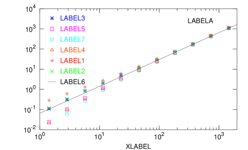
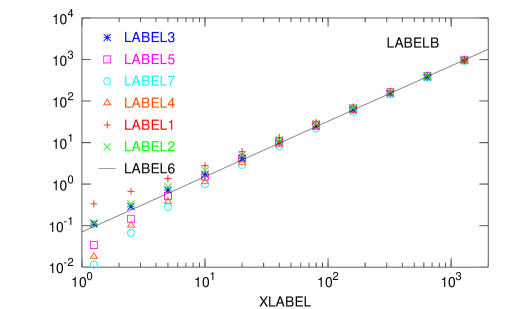
Figure 1: Measured variances and covariances of the quantities $X_{L+}$, $X_{R+}$, $X_{L-}$, and $X_{R-}$ for (a) $\epsilon=0.4$ $(b=1.75)$ and (b) $\epsilon=-0.6$ $(b=0.75)$. $\langle AB\rangle_{c}$ denotes $\langle AB\rangle-\langle A\rangle\langle B\rangle$. Note that because of the left-right symmetry some of the possible combinations are equal to each other. The simulation parameters are $N=1600$, 10000 realizations and equilibration times (see below) $t_{\mathrm{equil}}=14286$ (a), $t_{\mathrm{equil}}=12500$ (b).

The scaling ansatz (12) predicts for $1<b<3$ that the variance $\sigma^{2}$ of the distance $x(t)=X_{L+}(t)+X_{R+}(t)-X_{L-}(t)-X_{R-}(t)$ between the two probes increases with a lower power of $t$, namely, $\sigma^{2}\propto t^{(3-b)/z}$. This requires the cancellation of the leading term contribution of $\sigma^{2}$, which is in agreement with the results of the numerical simulations presented in figure 1(a), where the amplitudes of all the variances and covariances appear to be the same.

The mean distance is predicted to grow as $t^{(2-b)/z}$ for $1<b<2$. This is confirmed by Monte Carlo data presented in figure 2 for some values of $b$ in this range. At $b=2$ $(\epsilon=0.8)$ the mean distance is predicted to grow logarithmically in time. Our numerical simulations for this case show that the mean distance remains very small (of the order of a few lattice constants) in the time interval which was studied, and it grows slowly in time.

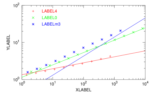
Figure 2: Average distance of the two probes as a function of $t$ for some values of $\epsilon$. Solid lines indicate the predicted behaviour for large $t$. The data are shown on a log-log scale. The simulation parameters are $\epsilon=0.4$: $N=1000$, $t_{\mathrm{equil}}=14286$, and 64000 realizations; $\epsilon=0$: $N=7000$, $t_{\mathrm{equil}}=100000$, and 64000 realizations; $\epsilon=-0.3$: $N=1600$, $t_{\mathrm{equil}}=15385$, and 24160 realizations.

To complete our analysis we measured the cumulative distribution function

$$\tilde{P}(x,t)=\mathrm{Prob}(\mbox{distance between the two probes }>x\mbox{ at time }t).$$ (14)

For this quantity, the scaling ansatz (12) yields

$$\tilde{P}(x,t)=t^{(1-b)/z-\beta}F(xt^{-1/z}),$$ (15)

where $F(y)=\int_{y}^{\infty}\eta^{-b}f(\eta)d\eta$. Consequently, in the case of $b>1$, $F(y)$ is expected to behave as $y^{-b+1}$ for small $y$, whereas $b<1$ implies $F(0)=1$.

The results for the scaling ansatz for the distribution function are shown in figure 3, where the quantity $\tilde{P}(x,t)t^{\frac{2}{3}(b-1)}$ is plotted against $xt^{-2/3}$ for some values of $b>1$. The data collapse shows that in this regime the scaling ansatz is correct with $z=3/2$ and $\beta=0$. On the other hand for $0<b<1$ no good data collapse is found. This may be understood by noting that at $b=0$ the leading quadratic nonlinearity in the KPZ equation vanishes and one is left with a quartic nonlinearity. According to standard wisdom, power counting shows that such a nonlinear term is irrelevant in the renormalization group sense. One expects a dynamical Edwards-Wilkinson exponent $z=2$, even though the fluid is driven. This results in strong crossover effects for small $b$, making the scaling form (15) with $z=3/2$ invalid. Measurements of the fluctuations of the individual probe particles (not shown in this paper) are found to be consistent with $z=2$.

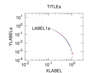
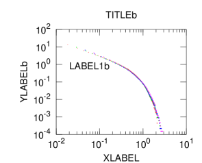
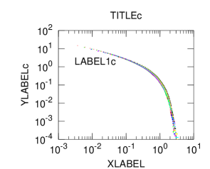
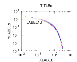
Figure 3: Simulation results for the KPZ fluid with two probes. The cumulative distribution function $\tilde{P}(x,t)$ of the distance between the two probes is measured and the quantity $\tilde{P}(x,t)t^{\frac{2}{3}(b-1)}$ is plotted against $xt^{-2/3}$ for some values of the parameter $\epsilon$. The simulations were carried out using an efficient multispin coding algorithm. The simulation parameters are: (a) $N=1600$, $t_{\mathrm{equil}}=11111$, $t=142,284,569,1138$ and 163712 realizations; (b) $N=1000$, $t_{\mathrm{equil}}=14286$, $t=91,183,366,731$ and 64000 realizations = 64000; (c) $N=7000$, $t_{\mathrm{equil}}=100000$, $t=128,256,1024,2048,4096,8192$ and 64000 realizations; (d) $N=1600$, $t_{\mathrm{equil}}=15385$, $t=197,394,788,1575$ and 24160 realizations.

A subtle point of the simulation is the proper choice of the initial condition. We simulated the process on a ring of $N$ (even) sites with equal ($N/2-1$) number of $+$ and $-$ particles and two probes. Initially the two probes were placed on neighbouring sites and any configuration of the remaining $N-2$ particles was chosen with equal probability. The process (1) was then simulated up to some time $t_{\mathrm{equil}}$ with the modification that the two probes are constrained to remain nearest neighbours, i.e., these particles hop together as if they occupied only a single site. During this “equilibration” the fluid approaches its stationary structure in the vicinity of the probes up to a distance of the order $t_{\mathrm{equil}}^{2/3}$. At this point, defined as $t=0$, the restriction for the relative position of the probes is released and the distance between the two probes is measured. In our analysis we consider $t\ll t_{\mathrm{equil}}$ so that the probe particles always move within an equilibrated region.

Clearly, there are also other relevant choices for the initial condition, which describe different physical scenarios. For example one may consider an initial state obtained by letting the two probes move freely and $t=0$ is defined as the time they first meet after some equilibration time. This case is not studied here. We believe that such a change in the initial condition will not change the scaling exponent, although it may result in a different scaling function. In order to test this statement we carried out Monte Carlo simulations of the $\epsilon=0$ case with equal number of $+$ and $-$ particles. The initial configuration was picked randomly with uniform probability conditioned on having the two probes on neighbouring sites. This initial state is equivalent to the above studied one with $t_{\mathrm{equil}}=0$. Results of the simulations (not presented here) yield the same scaling exponent $z=3/2$ as before, but the scaling function is different from the one in figure 3.c.

For more than two probes our dynamical scaling approach suggests the following scaling form for the joint distribution:

$$P(x_{1},x_{2},\cdots,x_{M})=x_{1}^{b}x_{2}^{b}\cdots x_{M}^{b}t^{-M\beta}P(x_{1}t^{-\frac{1}{z}},x_{2}t^{-\frac{1}{z}},\cdots,x_{M}t^{-\frac{1}{z}})$$ (16)

for $M+1$ probes with $z=3/2$. Here the formation of bound states for $b>2$ leads to a condensation transition for a finite density of probes. This phase transition was discussed in [10].

4 Probe particles with mixed dynamics

In this section we consider the model of a cluster with mixed dynamics and study its temporal evolution. In particular we are interested in the growth law governing the length of the cluster. As is evident from the definition of the model, two processes control the dynamics of a cluster of length $x$: at both ends there is (a) a growth process with rate $j_{0}(\epsilon)$, and (b) a length decreasing process with rate $1$, see (8-10). To analyze the dynamics of the cluster length we introduce processes for the individual motion of the probes as defined above. The growth process at both ends is a Poisson process and hence uncorrelated in time. Thus $\langle X_{R+}(t)\rangle=\langle X_{R+}^{2}(t)\rangle-\langle X_{R+}(t)\rangle^{2}=j_{0}t$ and similarly for $X_{L+}$.

The length decreasing processes, $X_{R-}(t)$ and $X_{L-}(t)$ are correlated in time through the dynamics of the particles within the cluster. Therefore the process $x(t)$ is also non trivially correlated in time. The mean rate of change of the length decreasing process, ${\rmd/\rmd t}{\langle X_{R-}(t)+X_{L-}(t)\rangle}=2j_{x}^{\rm out}$, depends on $x$ (5).

We start the analysis of $x(t)$ by demonstrating that the dynamical exponent of this process is $z=2$. As before, we measure the variances and covariances of $X_{R\pm}(t)$ and $X_{L\pm}(t)$. We find that for all these quantities the asymptotic growth is linear in $t$. In combining these expressions to calculate $\sigma^{2}$ the leading order terms cancel for $b>1$ and the growth of $\sigma^{2}$ becomes sub-linear, just like in the case of the KPZ fluid. The fluctuations of the motion of the probe particles are thus determined by the fluctuations of the uncorrelated incoming current (see figure 4). The temporal behaviour of the average distance between the probes for various values of $\epsilon$ is given in figure 5. The measured value of the growth exponent $\nu$ obtained from equation (13) is consistent with dynamical exponent $z=2$.

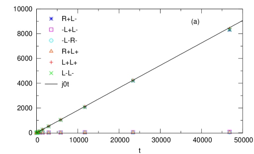
Figure 4: Measured variances and covariances of the quantities $X_{L+}$, $X_{R+}$, $X_{L-}$, and $X_{R-}$ in the mixed model for (a) $\epsilon=0.4$ $(b=1.75)$ and (b) $\epsilon=-0.6$ $(b=0.75)$. $\langle AB\rangle_{c}$ denotes $\langle AB\rangle-\langle A\rangle\langle B\rangle$. Note that because of the left-right symmetry some of the possible combinations are equal to each other. The averages were taken over 10000 realizations.

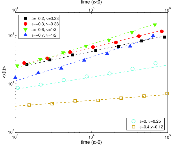
Figure 5: Results of numerical simulations for the average distance $\langle x(t)\rangle$ between the probes for various values of $b$. Lines are drawn with a slope as expected from equation 13.

In characterizing the dynamics of the two probes one may argue that they can be considered as two coupled random walkers. The driven fluid in between the probes generates an effective interaction, thus reducing the model to a two-particle problem. These particles hop away from each-other with a constant rate $j^{\rm in}$ of (7). On the other hand the rate at which they hop towards each-other, $j^{\rm out}_{x}$ , depends on the distance $x$ between them according to (5). This description neglects the fact that the two-particle process is not memoryless and leads to a reduced master equation for the interparticle distance, which can be transformed into a Fokker-Planck equation in a continuum limit. This approach was taken in reference [9] and the resulting scaling forms for the distance distribution were calculated. Here we compare this analytical result with simulations of the mixed model. In the full range of $b<2$ we obtain good data collapse with a dynamical exponent $z=2$, which is consistent with the Fokker-Planck approach, see figure 6. However, For $b<1$ the scaling function does not seem to agree with the Fokker-Planck prediction of reference [9]. We have no explanation for this discrepancy.

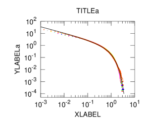
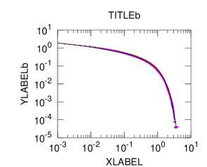
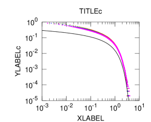
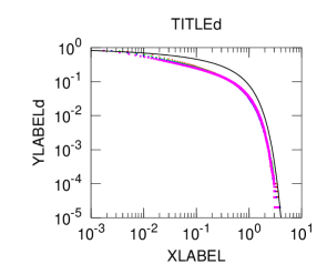
Figure 6: Simulation results for the mixed model. The cumulative distribution function $\tilde{P}(x,t)$ of the distance between the two probes is measured and the quantity $\tilde{P}(x,t)t^{\frac{1}{2}(b-1)}$ (for $b>1$) and $\tilde{P}(x,t)$ (for $b<1$) is plotted against $xt^{-1/2}$ for some values of the parameter $\epsilon$. The solid line indicates the prediction of the Fokker-Planck equation which is in good agreement with the data collapse for $b>1$. The simulation parameters are: (a) $t=4096,8192,16384,32768,65536,131072,262144,524288$; (b) $t=46811,93622,187246,374491$; (c) $t=43691,87381,174763,349525$; (d) $t=40960,81920,163840,327680$; and 50000 realizations for each case

An interesting generalization of the mixed model is obtained by allowing for probe particles between the fluctuating boundaries of the system. These extra probes have the same dynamics as the $0$ particles in the KPZ fluid (1) while the evolution at the boundaries is unchanged (8-10). Here the extra probes divide the system into several clusters. Numerical simulations (not presented here) show that the evolution of these clusters is described by the same dynamical exponent $z=2$ as for the case of no intermediate probes. We measured the quantities $X_{L+},X_{R+},X_{L-},X_{R-}$ in a simulation for intermediate clusters and the result is very similar to those shown in figure 4. Thus the uncorrelated noise acing on the boundaries dominate the entire system, including the inner probes which are not affected directly by it. These results suggest a scaling form similar to (16) with $z=2$ for a system with $M$ clusters ($M-1$ inner probes).

5 Conclusions

In this paper the dynamics of two probe particles embedded in a one dimensional driven fluid is studied. The non-equilibrium dynamics of the fluid generates an effective interaction between the probes. A simple model is introduced to study this dynamics. Within the framework of this model, sufficiently strong attraction between the fluid particles leads to a bound state of the probe particles. For less pronounced attraction (or repulsion) a weakly bound state is found in which the average distance between the probes grows algebraically with time, with a non-universal growth exponent. The probes become unbound for sufficiently strong repulsion of the fluid particles, leading to dynamics characterized by a universal growth exponent determined by the dynamical exponent $z$ of the fluid.

In previous work by some of the authors of the present paper [9] a similar analysis was performed using a Fokker-Planck approach, implying a dynamical exponent $z=2$. Here we argue that this analysis does not apply to the KPZ fluid which was envisaged in [9]. In order to clarify the validity of that analysis, two cases which lead to different dynamical exponents are considered here.

In the first case the probe particles are embedded in a KPZ like fluid. Here the dynamical exponent which determines the motion of the probes is predicted to be the KPZ exponent $z=3/2$. This is verified by numerical studies.

In the second case the system is coupled to an external driving force which is temporally uncorrelated. This leads to mixed dynamics where both the temporally correlated noise generated by the KPZ fluid and the uncorrelated external noise drive the motion of the probes. Here we observe numerically that the dynamical exponent is $z=2$. In this case the analysis of [9] applies in the range $b>1$.

The different dynamical exponents of the two models can be traced back to the fluctuations of the incoming and outgoing currents. We observe that in both cases the exponent is determined by the incoming current. This result is found to hold when the two models are generalized to include any finite number of probe particles. It would be interesting to understand how the interplay of the correlated and the uncorrelated noise in the mixed model generates $z=2$. Also the crossover behaviour for $b<1$ that leads to poor scaling collapse in the KPZ case is an intriguing open problem.

References

References

- [1] B. Widom, J. Chem. Phys. 39, 2808 (1963).
- [2] T.M. Liggett, Stochastic Interacting Systems: Voter, Contact and Exclusion Processes, (Springer, Berlin, 1999).
- [3] G.M. Schütz in Phase Transitions and Critical Phenomena vol 19, ed. C. Domb and J. Lebowitz (Academic, London, 2001).
- [4] J.M. Burgers The Non Linear Diffusion Equation (Reidel, Boston, 1974)
- [5] M. Kardar, G. Parisi and Y. Zhang, Phys. Rev. Lett. 56, 889 (1986).
- [6] P. Ferrari, Ann. Prob. 14, 1277 (1986); A. De Masi, C. Kipnis, E. Presutti and E. Saada, Stoch. Stoch. Rep. 27, 151 (1989); P. Ferrari, C. Kipnis and E. Saada, Ann. Prob. 19, 226 (1991).
- [7] B. Derrida, S.A. Janowsky, J.L. Lebowitz, and E.R. Speer, Europhys. Lett. 22, 651 (1993); J. Stat. Phys. 73, 813 (1993); B. Derrida, J.L. Lebowitz, and E.R. Speer, J. Stat. Phys. 89, 135 (1997).
- [8] Y. Kafri, E. Levine, D. Mukamel, G.M. Schütz, and J. Török, Phys. Rev. Lett. 89, 035702 (2002).
- [9] E. Levine, D. Mukamel, and G.M. Schütz, Europhys. Lett. 70, 565 (2005).
- [10] Y. Kafri, E. Levine, D. Mukamel, G.M. Schütz, and R.D. Willmann, Phys. Rev. E 68, 035101 (2003).
- [11] C. Godrèche, E. Levine and D. Mukamel, J. Phys. A: Math. Gen. 38, L523-L529 (2005).
- [12] S. Katz, J.L. Lebowitz, and H. Spohn, J. Stat. Phys. 34, 497 (1984).
- [13] V. Popkov and G.M. Schütz, Europhys. Lett 48, 257 (1999); J.S. Hager, J. Krug, V. Popkov, and G.M. Schütz, Phys. Rev. E 63, 056110 (2001).
- [14] M.R. Evans, E. Levine, P.K. Mohanty, and D. Mukamel, Euro. Phys. J. B 41, 223 (2004).
- [15] G. Schütz and E. Domany J. Stat. Phys. 72, 277 (1993); B. Derrida, V. Hakim, M.R. Evans, and V. Pasquier J. Phys. A 26, 1493 (1993).
- [16] J. Krug and P. Meakin, J. Phys. A 23, L987, (1990).
- [17] H. van Beijeren, R. Kutner and H. Spohn, Phys. Rev. Lett. 54, 2026 (1985).