Spin Liquid States on the Triangular and Kagomé Lattices: A Projective Symmetry Group Analysis of Schwinger Boson States

Abstract

A symmetry based analysis (Projective Symmetry Group) is used to study spin liquid phases on the triangular and Kagomé lattices in the Schwinger boson framework. A maximum of eight distinct $Z_{2}$ spin liquid states are found for each lattice, which preserve all symmetries. Out of these only a few have nonvanishing nearest neighbor amplitudes which are studied in greater detail. On the triangular lattice, only two such states are present - the first (zero-flux state) is the well known state introduced by Sachdev, which on condensation of spinons leads to the 120 degree ordered state. The other solution which we call the $\pi$-flux state has not previously been discussed. Spinon condensation leads to an ordering wavevector at the Brillouin zone edge centers, in contrast to the 120 degree state. While the zero-flux state is more stable with just nearest-neighbor exchange, we find that the introduction of either next-neighbor antiferromagnetic exchange or four spin ring-exchange (of the sign obtained from a Hubbard model) tends to favor the $\pi$-flux state. On the Kagomé lattice four solutions are obtained - two have been previously discussed by Sachdev, which on spinon condensation give rise to the $q=0$ and $\sqrt{3}\times\sqrt{3}$ spin ordered states. In addition we find two states with significantly larger values of the quantum parameter at which magnetic ordering occurs. For one of them this even exceeds unity, $\kappa_{c}\approx 2.0$ in a nearest neighbor model, indicating that if stabilized, could remain spin disordered for physical values of the spin. This state is also stabilized by ring exchange interactions with signs as derived from the Hubbard model.

I Introduction

Recent experiments on frustrated quantum magnets with unusual properties Coldea (2003); Kanoda (2003); Masutomi (2004); Helton (2006) has revived interest in spin liquid phases. At the same time the theoretical understanding of spin liquid phases in $D>1$ has also matured over the last few years - for example it is now established that such states are typically accompanied by emergent gauge fields in their deconfined phase. Simple and tractable lattice Hamiltonians that realize these phases can also be constructed. Nevertheless, there is still a pressing need to understand the situations in which microscopic spin models might exhibit such phases, and the variety of such phases and their phenomenological properties.

The triangular lattice antiferromagnet has been considered a good place to look for such spin liquid states, its geometry is considered less conducive to magnetic order than for example the square lattice antiferromagnet, and more recently there has been evidence from numerical calculations Misguich (1999); Sorella: ; Sheng: ; Singh: especially in the presence of anisotropic interactions and ring exchange, for unconventional physics. Similarly, recent experiments on quantum magnets with a triangular lattice structure - Cs₂CuCl₄ Coldea (2003), $\kappa$-(ET)₂Cu(CN)₃Kanoda (2003) and ³He films adsorbed on graphiteMasutomi (2004) show unusual properties that may be interpreted in terms of spin liquid phases or proximity to such a state. While the spin gapped $Z_{2}$ spin liquid states considered in this paper are probably not appropriate to directly describe these experimental systems, except perhaps at the very lowest temperatures, they motivate a closer study of possible spin liquid states on the triangular lattice. The highly frustrated Kagomé lattice has long been considered a good system for realizing exotic ground states. While there are fewer experimentally well studied examples of quantum spins on the Kagomé lattice, conventional semiclassical analysis fails to produce a unique ground state when applied to this frustrated lattice. Hence, spin disordered states like spin liquids may be realized.

In describing spin liquid states of quantum magnets, two distinct approaches have been found to be useful. The first involves writing the quantum spin (e.g. spin-1/2) as a fermion bilinear (fermionic spinons), and imposing a constraint on the total number of fermions on each site. This fermionic approach is analytically pursued by writing down a mean field ansatz where the constraint is imposed only on average to begin with. This mean field theory may also be viewed as a source of variational wave-functions, which after projection yields spin wave functions. An important step in understanding the variety of spin liquid states possible in this representation was taken by Wen and collaboratorsWen (2002, 2002); Zhou (2003) who introduced the Projective Symmetry Group (PSG) classification of spin liquids that respect the microscopic symmetries of the system. This provides a guide to identifying the correct gauge group describing the spin liquid (if it survives projection) and also allows for a further classification of different spin liquid phases with the same gauge group. These different spin liquid phases differ in subtle ways from one another, for example in terms of the location of the wavevector of their lowest energy spin-1 excitation. The advantage of such classification is that it allows for an exploration of possible spin liquid states independent of specific Hamiltonians that might realize them as ground states. In this way the symmetric spin liquid states within the fermionic spin representation on the square and triangular lattices were classified Wen (2002); Zhou (2003).

A different way to describe spin liquids is via the Schwinger boson approach, where the spin operator is written as a boson bilinear (bosonic spinons) and was analyzed using a large-N approach Arovas (1988); Read (1991); Sachdev (1991, 1992) . An advantage of this approach is that it is able to readily access both spin liquid states as well as conventional magnetically ordered states, which arise from the condensation of the Schwinger bosons. For instance, in the case of the triangular latticeSachdev (1992), Sachdev found a spin liquid state which on decreasing the strength of quantum fluctuations to the size expected for s=1/2, gave way to the 120 degree magnetically ordered state, expected of classical spins on this lattice. However the possibility of other Schwinger boson spin liquid states on the triangular lattice have not been systematically explored. Similarly, on the Kagomé lattice, Sachdev Sachdev (1992) found two solutions, which on spinon condensation gives rise to $\sqrt{3}\times\sqrt{3}$ or the $q=0$ magnetically ordered states.

Mapping out the possible spin liquid states on these lattices is of interest for two reasons. First, when attempting to identify a candidate spin liquid state to match with experimental data or numerical simulations, one needs to specify precisely what the nature of the state is, and the quantum numbers of its excitations. Therefore while the simplest spin liquid may fail to match these details, other spin liquid states may give different predictions. Second, there may exist solutions stabilized with different interactions which remain spin liquids even for physical values of the spin. This would be particularly appealing as it would also provide direction to the search for spin liquid states. Even when the system is in the ordered phase, if it is proximate to a critical point where spin liquid physics holds, it has been argued IsakovSenthilKim that finite energy and finite temperature signatures of this will be unusual and best described in terms of the spin liquid variables. Therefore, a systematic investigation of the possible solutions of the Schwinger bosons states is required on the lines of the PSG analysis of the fermionic spin liquid states. This will also shed light on the connection between two approaches, for example, which states can be described in one but not the other approach.

In this paper we will adapt the technique of Projective Symmetry Groups, developed by Wen and collaboratorsWen (2002, 2002); Zhou (2003) in the context of fermionic mean field theories to study Schwinger boson mean field theories. We will focus on the triangular and Kagomé lattices, in particular on spin liquid states with the Ising gauge group ($Z_{2}$ gauge theories) which preserve the microscopic spin symmetries. Surprisingly, the number is not large (less than or equal to 8 for both lattices), which includes, in addition to the solution found by Sachdev, a set of fundamentally different mean field wave functions, which give rise to $Z_{2}$ spin liquids. In particular, if we make the further reasonable assumption of restricting to states with non-trivial nearest-neighbor bond amplitudes, there is only one other state on the triangular lattice, which we call the $\pi$-flux state. Similarly, on the Kagomé lattice, $Z_{2}$ spin liquid states with nonvanishing nearest neighbor bond amplitudes, include, in addition to the two states found by Sachdev, two additional states, which we refer to as the [$\pi$ Hex,$\pi$ Rhom] and [$0$ Hex,$\pi$ Rhom] (which specifies the flux in the length-six hexagonal loop, and the length-eight rhombus). One of the problems in searching for spin liquid states has been the tendency of various spin Hamiltonians to yield magnetically order states, which is reflected in the small values of $\kappa_{c}$, the critical quantum parameter at which spin ordering occurs in the Sachdev states: $\kappa_{c}\approx 0.3$ on the triangular, and $\kappa_{c}\approx 0.5$ for the Kagomé states in large-NSachdev (1992). (Note, $\kappa=2S$ in the case of spin $S$ but it is convenient to extend it to take on all real values). A feature of the new states that is their relative stability against magnetic order which is seen in the larger critical quantum parameter at which spin ordering occurs: $\kappa_{c}\approx 0.75$ for the pi-flux triangular state, and $\kappa_{c}\approx 0.9$ and $\kappa_{c}\approx 2.0$ for the two new Kagomé states respectively, in nearest neighbor models.

While the distinct mean field solutions of the PSG analysis are typically local minima of the mean field energy, an important question is whether they can be stabilized as global minima with appropriate interactions. This is discussed in detail for the case of the triangular lattice in this paper. While the zero-flux state is stabilized with just nearest-neighbor antiferromagnetic spin couplings, introducing next neighbor antiferromagnetic couplings or ring exchange (of the sign arising from the Hubbard model) both tend to favor the $\pi$-flux state. We obtain the conditions on the microscopic spin interactions which favor this state and argue that this may be a fruitful parameter regime for numerical searches for spin liquids. In general we find that ring exchange on even length loops (with the sign as derived from the Hubbard model), favors states with $\pi$ flux on length-$4n$ loops, while it favors states with zero flux in length-($4n+2$) loops ($n$ is positive integer). This is in contrast to fermionic case where ring exchange disfavors fluxMotrunich (2004) for fermions in all loops. Addition or ring exchange on length-$6$ and length-$8$ loops can stabilize the [$0$ Hex,$\pi$ Rhom] state on the Kagomé, which is good spin liquid candidate since it has $\kappa_{c}=2.0$.

On spinon condensation, the triangular lattice $\pi$-flux state naturally leads to magnetically ordered states with wavevectors at the midpoints of the Brillouin zone edges (in contrast to the zero-flux state which leads to the 120 degree state with wavevector at the zone corners). This allows us to understand semi-classical (large spin) calculations in the presence of moderate-neighbor antiferromagnetic couplings or ”antiferromagnetic”, (with sign as obtained from the Hubbard model) ring exchange on the triangular lattice, where ordered states with the same wavevector are found. It is tempting to connect the possible ordered states on the triangular lattice as emerging from spin condensation out of the few Schwinger boson spin liquid states allowed by the PSG. New quantum transitions are expected on spinon condensation out of the spin liquid states obtained here, and will be the subject of future study.

Layout of the paper: In Section II we briefly review the Schwinger boson mean field theory. Section III analyzes possible spin liquid states on the triangular lattice. It first reviews the Projective Symmetry Group classification of spin liquid states and the strong constraints that arise from relations between symmetry group elements. This is then applied to Schwinger boson states on the triangular lattice. A new state is found, the $\pi$-flux state, which is further analyzed - in particular spin configurations resulting from spinon condensation are described, and Hamiltonians stabilizing this mean field solution are obtained. The general effect of ring exchange interactions on Schwinger boson mean field states is discussed. In Section VI possible spin liquid states on the Kagomé lattice are studied, and the properties of one of them, which is unusually stable against spin ordering, is described in more detail. The PSG analysis and other details are relegated to the appendices, which also contains analysis for other lattices of interest such as the anisotropic triangular lattice.

II Schwinger Boson Mean Field Theory

There are a variety of ways of formulating the Schwinger boson mean field theory, for example, as a large-N approach Arovas (1988); Read (1991), or as an approximate variational approach.

Here we will formulate a variational approach that will provide us with a unified way to study the effect of different interactions. We write the spin Hamiltonian:

$$H=J_{1}\sum_{\langle ij\rangle}\mathbf{S}_{i}\cdot\mathbf{S}_{j}+J_{2}\sum_{\langle\langle ij\rangle\rangle}\mathbf{S}_{i}\cdot\mathbf{S}_{j}+\cdots$$ (1)

in terms of Schwinger bosons:

$$\mathbf{S}_{i}\cdot\mathbf{S}_{j}=\frac{1}{4}b^{\dagger}_{i\,\sigma}\mathbf{\sigma}_{\sigma,\sigma^{\prime}}b_{i\,\sigma^{\prime}}\cdot b^{\dagger}_{j\,\tau}\mathbf{\sigma}_{\tau,\tau^{\prime}}b_{j\,\tau^{\prime}}$$ (2)

with the constraint that at every site:

$$\sum_{\sigma}b^{\dagger}_{i\,\sigma}b_{i\,\sigma}=\kappa$$ (3)

where for a spin system with spin $S$, $\kappa=2S$. In the analysis below, it will be convenient to consider $\kappa$ to be a continuous parameter, taking on any non-negative value.

We now consider a variational approach to finding the ground states and excitations of (1). Motivated by the operator identity

$$\mathbf{S}_{i}\cdot\mathbf{S}_{j}=:\hat{B}_{ij}^{\dagger}\hat{B}_{ij}{{}^{\vphantom{\dagger}}}:-\hat{A}_{ij}^{\dagger}\hat{A}_{ij}{{}^{\vphantom{\dagger}}}$$ (4)

where $:\,:$ is normal ordering, and operators $\hat{A}$ and $\hat{B}$ are defined as

$$\hat{B}_{ij} = \frac{1}{2}\sum_{\sigma}b_{i\sigma}^{\dagger}b_{j\sigma}{{}^{\vphantom{\dagger}}}$$ (5)

$$\hat{A}_{ij} = \frac{1}{2}\sum_{\sigma,\sigma^{\prime}}\epsilon_{\sigma\sigma^{\prime}}b_{i\sigma}b_{j\sigma^{\prime}}$$ (6)

we consider a ”Mean Field” Hamiltonian which is quadratic in terms of the Schwinger bosons,

$$H_{MF} = \sum_{ij}J_{ij}(-A_{ij}^{*}\hat{A}_{ij}+B_{ij}^{*}\hat{B}_{ij}+{\rm h.c.})$$ (7)

$$+\sum_{ij}{{J_{ij}}(A_{ij}^{*}A_{ij}-B_{ij}^{*}B_{ij})}$$

$$-\mu\cdot\sum_{i}{\left(\sum_{\sigma}{b_{i\sigma}^{\dagger}b_{i\sigma}}{{}^{\vphantom{\dagger}}}-\kappa\right)}$$

where complex numbers $A_{ij}{{}^{\vphantom{\dagger}}}=-A_{ji}{{}^{\vphantom{\dagger}}},\,B_{ij}{{}^{\vphantom{\dagger}}}=B_{ji}^{*}$ are the parameters of the mean field ansatz.

In the large-N $Sp(N)$ theory, the mean field Hamiltonian contains only the large-N generalization of the $A$ term. However, since both $A$ and $B$ terms are consistent with global $SU(2)$ symmetry (global spin rotation symmetry) they are both included in the current theory. The introduction of both terms can be found in Gazza Gazza (1993) and many other papers Lefmann (1994); Misguich (1998).

This Hamiltonian is used to generate a variational wavefunction in terms of the variational parameters $|\Psi(A_{ij},\,B_{ij},\mu)\rangle$. In order to obtain a spin wavefunction, we need to project $|\Psi\rangle$ into the constrained Hilbert space where the total number of bosons at each site is exactly $2S$. Strictly speaking one must evaluate variational energies after this projection step, using the spin Hamiltonian (1). This generalization of Gutzwiller projection to Schwinger boson has been studied by Chen and collaboratorsChenYC (1993); ChenYC-Xiu (1993). However, since this hard projection is not possible to implement analytically (it is even difficult to do numerically) we rely on a approximate strategy that forgoes implementing the constraint locally, but only on the average - i.e. we tune $\mu$ to ensure that:

$$\sum_{\sigma}{\langle b^{\dagger}_{i\,\sigma}b_{i\,\sigma}\rangle}=\kappa$$ (8)

we then evaluate the expectation value of the Hamiltonian (2), written out in terms of Schwinger bosons (2) using the variational wavefunction. The resulting variational energy is then minimized with respect to the variational parameters $A_{ij},\ B_{ij}$. This yields the self-consistent equations,

$$\langle\hat{A}_{ij}\rangle=A_{ij},\,\quad\langle\hat{B}_{ij}\rangle=B_{ij}$$ (9)

When these self-consistent equations are satisfied, the variational(mean field) energy is simply obtained by utilizing the following identity,

$$\langle\mathbf{S}_{i}\cdot\mathbf{S}_{j}\rangle=\frac{3}{2}\left(|B_{ij}|^{2}-|A_{ij}|^{2}\right)$$ (10)

The effect of projection on energetics will be a topic of future study.

III PSG for Schwinger Boson States on the Triangular Lattice

We would like to classify Schwinger boson mean field states available to us on the triangular lattice in terms of the distinct spin liquid phases they can give rise to. This exercise allows us to readily obtain potentially interesting states relevant to quantum spin systems on the triangular lattice. Interactions that stabilize these states are discussed subsequently.

This classification follows the classification of fermionic mean field states in Wen (2002, 2002); Zhou (2003). Here however the underlying local transformation is $U(1)$ (not $SU(2)$ as in the case of fermions). For mean field theories that survive projection (or equivalently, survive fluctuations) to give rise to a spin liquid state, this procedure classifies the distinct quantum phases of the system. We will require that the mean field theory reflects the underlying microscopic symmetries of the spin model. This leads to symmetric spin liquid states. The symmetry transformations include the space group (lattice translations and point group symmetries) of the triangular lattice, spin rotation symmetry and time reversal symmetry. The novel ingredient here is that the mean field state may preserve these symmetries in some indirect way. In addition to the symmetries of the original spin model, one also finds an extra global symmetry in all the mean field ansatz which is a subset of the local $U(1)$ transformations mentioned previously. This is called the Invariant Gauge Group (IGG) in the terminology of Ref. Wen (2002). Since we are interested in mean field states that have exactly the same symmetry as the underlying spin model, not less or more, this is to be identified with the gauge group of the emergent gauge theory. In the examples below we will find an extra $Z_{2}$ symmetry in the mean field ansatz, hence the spin liquids that are obtained with this procedure are $Z_{2}$ spin liquids, but with different internal structures depending on how the microscopic symmetries of the lattice model are realized. Thus, in contrast to conventional states which are distinguished by patterns of broken symmetry, spin liquid phases that are completely symmetric and even share the same gauge group can be further distinguished in terms of how the symmetries are realized.

In Schwinger boson representation of spins, there is a local $U(1)$ transformation of bosons:

$$b_{{\mathbf{r}}\sigma}\rightarrow e^{{i}{\phi}({\mathbf{r}})}b_{{\mathbf{r}}\sigma}$$ (11)

which leaves all physical observables unchanged. Under this transformation, our mean field ansatz ($A_{ij}$, $B_{ij}$) also transform:

$$A_{ij} \rightarrow e^{-{i}{\phi}(i)-{i}{\phi}(j)}A_{ij}$$ (12a)

$$B_{ij} \rightarrow e^{+{i}{\phi}(i)-{i}{\phi}(j)}B_{ij}$$ (12b)

Two mean field ansatz that are related by such a transformation, give rise to the same spin wave function after projection. However, we will be interested in a class of transformations that leave the mean field ansatz invariant. Naively, one might expect that since we are interested in states that maintain all the microscopic symmetries, the mean field ansatz should be invariant under their operation (e.g. lattice translations). While this is a sufficient condition for invariance, it is not a necessary one, due to the presence of the local $U(1)$ transformations described above. A symmetry operation might return the ansatz to a $U(1)$ transformed form which would suffice, since the same spin wavefunction will be obtained on projection. Hence symmetry transformations that leave the Ansatz invariant in general will contain the naive transformation combined with a local $U(1)$ transformation. The set of all transformations that leave a mean ansatz invariant is called the Projective Symmetry Group (PSG) Wen (2002). In principle, we would like to associate each and every element of this group with a physical symmetry. This is because if the mean field ansatz is to be a faithful representation of the microscopic physics, it should have exactly as much symmetry as the original model. However, we always find that there are some elements of the PSG that are pure local transformation of the kind (11). The set of such elements also forms a group (a subgroup of the PSG) and is called the invariant gauge group (IGG). These cannot be the result of a physical symmetry. It is therefore natural to associate these elements with the emergent gauge group that describes the spin liquid phase obtained (if the mean field state survives projection). Therefore the first step is to identify the IGG of a mean field ansatz.

The Invariant Gauge Group for Schwinger Boson Mean Field Theories: A general Schwinger boson mean field Hamiltonian with explicit global $SU(2)$ symmetry (global spin rotation symmetry) must be of the form of equation (7).

It is clear that if $A_{ij}$ and $B_{ij}$ are both nonzero the IGG must be a $Z_{2}$ group. The only two elements of IGG are identity operation ${\rm\bf 1}$ and the IGG generator $-{\rm\bf 1}:\ b_{{\mathbf{r}}\sigma}\rightarrow-b_{{\mathbf{r}}\sigma}$. This can be seen by considering only one bond.

Note, that if $B_{ij}$ are nonzero while all $A_{ij}$ vanish, the IGG will be a $U(1)$ group: $b_{{\mathbf{r}}\sigma}\rightarrow e^{{i}{\phi}}b_{{\mathbf{r}}\sigma}$, where ${\phi}$ is a site-independent constant. However it is unlikely for this ansatz to describe an antiferromagnet according to (10). Finally we should consider the case with only non-vanishing $A_{ij}$. On a frustrated lattice the IGG will still be the above $Z_{2}$ group. However, if the lattice is bipartite, the IGG will be a $U(1)$ group: $b_{{\mathbf{r}}\sigma}\rightarrow e^{\pm{i}{\phi}}b_{{\mathbf{r}}\sigma}$, where we apply opposite signs on the two sublattices. This is the case of simple square lattice.

We will only consider PSGs with $Z_{2}$ IGG in the following discussion. Hence we are implicitly restricting ourselves to $Z_{2}$ spin liquid states, which are the natural spin liquid states on frustrated lattices within the Schwinger boson formalism.

III.1 Algebraic Constraints on the PSG

We consider mean field Hamiltonian that preserves all of the physical symmetries in the PSG sense (symmetric spin liquid states). They are spin rotation symmetry, lattice space group symmetries and time reversal symmetry. The spin rotation symmetry is already implemented by considering mean field ansatz of the form (7), which is explicitly invariant under global $SU(2)$ spin rotations. We will consider time reversal symmetry at the end of our derivation. The operations that we will now pay special attention to are the space group symmetries (translations and point group operations for the triangular lattice). As discussed before, these can be implemented via combining the naive transformation with a local (gauge) $U(1)$ transformation. One can ask the question - is it possible to have mean field ansatz with any choice of the gauge transformations? It turns out that there are algebraic relations among the symmetry group elements that strongly constrain the possible choices of gauge transformations. Thus, to obtain all possible PSGs we should first check the algebraic structure of PSGs without reference to a specific mean field ansatz. The possible PSGs allowed by the algebra of the space group are defined as the algebraic PSGs related to the space group.

For the isotropic triangular lattice, the space group is generated by two translations ${T_{1}}$ and ${T_{2}}$, one reflection ${\sigma}$ in a bond and the 60 degree rotation ${R_{\frac{\pi}{3}}}$ about a lattice site.

We use the following oblique coordinate system. In this system a site index ${\mathbf{r}}$ has two integer components ${\mathbf{r}}=(r_{1},r_{2})$.

Figure 1: Oblique coordinates system of triangular lattice.

Then the four generators are given by the following formulae

$${T_{1}}:\ (r_{1},\ r_{2}) \rightarrow (r_{1}+1,\ r_{2})$$ (13a)

$${T_{2}}:\ (r_{1},\ r_{2}) \rightarrow (r_{1},\ r_{2}+1)$$ (13b)

$${\sigma}:\ (r_{1},\ r_{2}) \rightarrow (r_{2},\ r_{1})$$ (13c)

$${R_{\frac{\pi}{3}}}:\ (r_{1},\ r_{2}) \rightarrow (r_{1}-r_{2},\ r_{1})$$ (13d)

For symmetric spin liquid states there must be four gauge group transformations ${G_{{T_{1}}}}$, ${G_{{T_{2}}}}$, ${G_{{\sigma}}}$, and ${G_{{R_{\frac{\pi}{3}}}}}$, such that the mean field ansatz is invariant under ${G_{{T_{1}}}}{T_{1}}$, ${G_{{T_{2}}}}{T_{2}}$, ${G_{{\sigma}}}{\sigma}$, and ${G_{{R_{\frac{\pi}{3}}}}}{R_{\frac{\pi}{3}}}$, respectively. We can represent the four gauge operations by their phase,

$${G_{X}}:\ b_{{\mathbf{r}}\sigma}\rightarrow e^{{i}{\phi_{X}}({\mathbf{r}})}b_{{\mathbf{r}}\sigma}$$ (14)

where the $X$ are ${T_{1}}$, ${T_{2}}$, ${\sigma}$, and ${R_{\frac{\pi}{3}}}$, respectively.

The PSG is generated by combining the generators of the IGG: $-{\rm\bf 1}$, and the above four compound operators ${G_{X}}X$.

The structure of the space group imposes algebraic constraints on the ${G_{X}}$. For instance, the combination of translations shown in FIG. 2 should be equivalent to the identity, i.e. ${T_{1}}^{-1}{T_{2}}{T_{1}}{T_{2}}^{-1}={\mathcal{I}}$. Therefore we require that the implementation of these symmetries in the PSG: $({G_{{T_{1}}}}{T_{1}})^{-1}{G_{{T_{2}}}}{T_{2}}{G_{{T_{1}}}}{T_{1}}({G_{{T_{2}}}}{T_{2}})^{-1}$ must be the equivalent of an identity operation, which means it is an element of the IGG, either ${\rm\bf 1}$ or $-{\rm\bf 1}$. This string can be rewritten as ${T_{1}}^{-1}{G_{{T_{1}}}}^{-1}{T_{1}}\cdot{T_{1}}^{-1}{G_{{T_{2}}}}{T_{1}}\cdot({T_{1}}^{-1}{T_{2}}){G_{{T_{1}}}}({T_{1}}^{-1}{T_{2}})^{-1}\cdot({G_{{T_{2}}}})^{-1}$. Using the fact that for a space group operation $Y$, the gauge transformation $(Y)^{-1}\cdot{G_{X}}\cdot Y$ acting on site ${\mathbf{r}}$ will just give a phase ${\phi_{X}}[Y({\mathbf{r}})]$ (where $Y(r)$ is the image of $r$ under the space group operation $Y$), we end up with the equation

$$\begin{split}&-{\phi_{{T_{1}}}}[{T_{1}}({\mathbf{r}})]+{\phi_{{T_{2}}}}[{T_{1}}({\mathbf{r}})]+{\phi_{{T_{1}}}}[{T_{2}}^{-1}{T_{1}}({\mathbf{r}})]-{\phi_{{T_{2}}}}({\mathbf{r}})\\ =&p_{1}\pi\end{split}$$ (15)

where $p_{1}\in\{0,1\}$ is independent of the site index ${\mathbf{r}}$, and arises from the fact that the identity operation can be any one of the two elements of the IGG.

Figure 2: An example of a relation between space group elements ${T_{1}}^{-1}{T_{2}}{T_{1}}{T_{2}}^{-1}={\mathcal{I}}$, that leads to an algebraic constraint on the PSG.

This kind of algebraic constraints strictly restrict the possible structures of PSG. It turns out (proof is in Appendix A) that there is only a finite set of such constraints, which if satisfied guarantees that all relations between space group elements are satisfied. These relations, beginning with the one described above, are:

$${T_{2}}{T_{1}} = {T_{1}}{T_{2}}$$ (16a)

$${T_{1}}{R_{\frac{\pi}{3}}} = {R_{\frac{\pi}{3}}}{T_{2}}^{-1}$$ (16b)

$${T_{2}}{R_{\frac{\pi}{3}}} = {R_{\frac{\pi}{3}}}{T_{1}}{T_{2}}$$ (16c)

$${T_{1}}{\sigma} = {\sigma}{T_{2}}$$ (16d)

$${T_{1}}{\sigma} = {\sigma}{T_{2}}$$ (16e)

$${R_{\frac{\pi}{3}}}^{-1} = [{R_{\frac{\pi}{3}}}]^{5}$$ (16f)

$${\sigma}^{-1} = {\sigma}$$ (16g)

$${R_{\frac{\pi}{3}}}{\sigma} = {\sigma}[{R_{\frac{\pi}{3}}}]^{5}$$ (16h)

These relations place severe constraints on the allowed PSGs. The most general solution that satisfies them is:

$${\phi_{{T_{1}}}}(r_{1},\ r_{2}) = 0$$ (17a)

$${\phi_{{T_{2}}}}(r_{1},\ r_{2}) = p_{1}\pi r_{1}$$ (17b)

$${\phi_{{\sigma}}}(r_{1},\ r_{2}) = p_{2}\pi/2+p_{1}\pi r_{1}r_{2}$$ (17c)

$$2{\phi_{{R_{\frac{\pi}{3}}}}}(r_{1},\ r_{2}) = p_{3}\pi+p_{1}\pi r_{2}(r_{2}-1+2r_{1})$$ (17d)

where $p_{1},\ p_{2},\ p_{3}$ are either 0 or 1. Thus there are at most eight distinct Schwinger boson symmetric spin liquid states on isotropic triangular lattice. If we put more conditions on the mean field ansatz (e.g. that the nearest-neighbor $A_{ij}$ are nonzero), then the number of possible symmetric spin liquid states is reduced from eight.

A detailed derivation of the above formulae is given in Appendix A. Also we include the solution of algebraic PSGs on the anisotropic triangular lattice.

III.2 From PSGs to Mean Field Hamiltonians :
Nearest-neighbor Models

If we assume that nearest-neighbor amplitudes $A_{ij}$ are nonzero, (which is natural given that nearest neighbor interactions in physical models tend to be dominant and usually antiferromagnetic), there are more constraints on the possible PSG structures.

This can be seen as follows. Since ${\sigma}$ maps bond $(0,0)\rightarrow(1,1)$ to itself, we must have ${\phi_{{\sigma}}}(0,0)+{\phi_{{\sigma}}}(1,1)=0\mod 2\pi$. This imposes the constraint $p_{2}=p_{1}\mod 2$. Also, bonds $(0,0)\rightarrow(-1,0)$ and $(0,0)\rightarrow(1,0)$ are related by a 180 degree rotation, $({R_{\frac{\pi}{3}}})^{3}$, and by antisymmetry and translation ${T_{1}}$ we have $A_{(0,0)\rightarrow(-1,0)}=-A_{(-1,0)\rightarrow(0,0)}=-A_{(0,0)\rightarrow(1,0)}$. This leads to another constraint

$$\begin{split}&{\phi_{{R_{\frac{\pi}{3}}}}}(-1,0)+{\phi_{{R_{\frac{\pi}{3}}}}}(0,1)+{\phi_{{R_{\frac{\pi}{3}}}}}(1,1)+3{\phi_{{R_{\frac{\pi}{3}}}}}(0,0)\\ =&\pi\mod 2\pi\end{split}$$

which fixes $p_{3}=1-p_{1}\mod 2$.

Thus we have only two non-equivalent PSGs, corresponding to $p_{1}=0$, which we call the zero-flux state or $p_{1}=1$ which we call the $\pi$-flux state.

1. The zero-flux state:

This state is specified in terms of the integers $p_{1}=0,\ p_{2}=0,\ p_{3}=1$, or equivalently in terms of the phase factors involved in implementing the space group operations:

$${\phi_{{T_{1}}}}(r_{1},\ r_{2})={\phi_{{T_{2}}}}(r_{1},\ r_{2})={\phi_{{\sigma}}}(r_{1},\ r_{2}) = 0$$

$${\phi_{{R_{\frac{\pi}{3}}}}}(r_{1},\ r_{2}) = \pi/2$$

We can now ask what mean field ansatz would be characterized by such a PSG. The mean field ansatz is specified by the amplitudes $A_{ij}$ and $B_{ij}$ on the various bonds. For this PSG, $B_{ij}$ and $A_{ij}$ on nearest-neighbor are both real and nonzero in general. Explicit expression for this ansatz are:

$$A_{(r_{1},r_{2})\rightarrow(r_{1}+1,r_{2})}=A_{(r_{1},r_{2})\rightarrow(r_{1},r_{2}+1)}$$

$$= -A_{(r_{1},r_{2})\rightarrow(r_{1}+1,r_{2}+1)}=A_{1},$$

$$B_{(r_{1},r_{2})\rightarrow(r_{1}+1,r_{2})}=B_{(r_{1},r_{2})\rightarrow(r_{1},r_{2}+1)}$$

$$= B_{(r_{1},r_{2})\rightarrow(r_{1}+1,r_{2}+1)}=B_{1}$$

The PSG predicts that next-nearest-neighbor $A$ must be zero. Since $A_{ij}=-A_{ji}$ is real and anti-symmetric, it is natural to represent it by oriented bonds. FIG. 3 is a pictorial representation of the ansatz for the zero-flux state.

Figure 3: Ansatz of the zero-flux state. An arrow from site $i$ to site $j$ means $A_{ij}>0$. All $A_{ij}$ have the same magnitude. All $B_{ij}$ are real and of uniform magnitude (not shown).

This ansatz has explicit translational invariance, and has been studied by Sachdev using the large-N method Sachdev (1992).

2. $\pi$-flux state:

This state is specified in terms of the integers $p_{1}=1,\ p_{2}=1,\ p_{3}=0$, or equivalently in terms of the phase factors involved in implementing the space group operations:

$${\phi_{{T_{1}}}}(r_{1},\ r_{2}) = 0$$

$${\phi_{{T_{2}}}}(r_{1},\ r_{2}) = \pi r_{1}$$

$${\phi_{{\sigma}}}(r_{1},\ r_{2}) = (\pi/2)+\pi r_{1}r_{2}$$

$${\phi_{{R_{\frac{\pi}{3}}}}}(r_{1},\ r_{2}) = \pi r_{1}r_{2}+(\pi/2)r_{2}(r_{2}-1)$$

The mean field ansatz that realizes this PSG is as follows. While the nearest-neighbor bond $A_{ij}$ is real and nonzero, the nearest-neighbor bond $B_{ij}$ must be zero. Expression of the ansatz is:

$$(-1)^{r_{2}}A_{(r_{1},r_{2})\rightarrow(r_{1}+1,r_{2})}=-A_{(r_{1},r_{2})\rightarrow(r_{1},r_{2}+1)}$$

$$= -(-1)^{r_{2}}A_{(r_{1},r_{2})\rightarrow(r_{1}+1,r_{2}+1)}=A_{1},$$

$$B_{(r_{1},r_{2})\rightarrow(r_{1}+1,r_{2})}=B_{(r_{1},r_{2})\rightarrow(r_{1},r_{2}+1)}$$

$$= B_{(r_{1},r_{2})\rightarrow(r_{1}+1,r_{2}+1)}=0$$

The PSG also predicts that the next-nearest-neighbor $B$ must be zero. Note, for this state the translation symmetry is not explicit in the Mean Field Hamiltonian, hence the unit cell for the Schwinger bosons is doubled. This $\pi$-flux ansatz for nearest-neighbor model is shown in FIG. 4.

Figure 4: Ansatz of the $\pi$-flux state. All nearest-neighbor $A_{ij}$ are real and of the same magnitude, and are positive in the directions shown. All nearest-neighbor $B_{ij}$ are zero. The unit cell for the Schwinger bosons is doubled due to the flux, and $u$ and $v$ are the two sites in this unit cell.

These two states can also be distinguished by the gauge-invariant phase of the product $A_{ij}{{}^{\vphantom{\dagger}}}(-A_{jk}^{*})A_{kl}{{}^{\vphantom{\dagger}}}(-A_{li}^{*})$, where $i,j,k,l$ form a rhombus with unit length sides. This quantity was introduced by Tchernyshyov, et. al. Tchernyshyov (2004) as the flux in the rhombus in bosonic large-N theory. Defining:

$$|A_{1}|^{4}e^{i\Phi}=A_{ij}{{}^{\vphantom{\dagger}}}(-A_{jk}^{*})A_{kl}{{}^{\vphantom{\dagger}}}(-A_{li}^{*})$$ (18)

where $|A_{1}|$ is the uniform magnitude of $A_{ij}$, we have that for the zero-flux state, the flux $\Phi=0$ for all rhombi; while for the $\pi$-flux state $\Phi=\pi$ for all rhombi. Therefore these two states are clearly not gauge equivalent mean field states.

Finally we can consider time reversal symmetry $\hat{T}$. Because the two ansatz are both real, they directly respect $\hat{T}$-symmetry, since time reversal transformation will change the ansatz to their complex conjugate. It is then an interesting question to ask what kind of PSG can support $\hat{T}$-breaking ansatz. It turns out that one must also break lattice reflection symmetry to obtain a time reversal breaking state. In Appendix. B we list the solutions of algebraic PSGs for anisotropic triangular lattice and the realizations in nearest-neighbor model which do support a $\hat{T}$-breaking ansatz.

IV Analysis of the Mean Field Theories

We now study the mean field theories arising from the ansatz described previously. Given the PSG classification, it follows that these different mean field solutions will be local minima of the mean field energy. In order to pick which of these is favored with a particular Hamiltonian, one needs to compare energies between these states, which is left to the next section. Here we content ourselves with describing the properties of each of these mean field ansatz. The discussion closely parallel Sachdev’s large-N solution of triangular lattice and Kagomé lattice Sachdev (1992). We also take the quantum parameter $\kappa$ as a continuous number, although for Schwinger bosons derived from $SU(2)$ spins of size $S$, $\kappa=2S$. For small $\kappa$, the spinon dispersion will be gapped and we have a spin liquid mean field ground state. When $\kappa$ goes beyond certain critical value $\kappa_{c}$ spinon dispersion becomes gapless, bosonic spinons condense, and magnetic long range order develops. For simplicity we present only the solution to the nearest-neighbor model.

IV.1 Zero-flux state

The mean field theory of this state is almost identical to Sachdev’s large-N theory for triangular lattice Sachdev (1992) and the phases obtained are continuously connected to the phases described in that work. The only difference is that we include the parameter $B_{ij}$, which is not present in the large-N treatment,and therefore our spinon dispersion and critical quantum parameter $\kappa_{c}$ differ slightly. This is reviewed briefly here before turning to a similar analysis of the $\pi$-flux state.

The Brillouin zone for the triangular lattice and our choice of coordinate systems in $\mathbf{k}$-space in shown in FIG. 5. In this oblique coordinates system, $\mathbf{k}\cdot{\mathbf{r}}=k_{1}r_{1}+k_{2}r_{2}$. For covenience we define $k_{3}=-k_{1}-k_{2}$.

Figure 5: Triangular Lattice Brillouin Zone (BZ) and $k$-space coordinate system. The large hexagon is the BZ of the original lattice and the zero-flux ansatz. The large rectangle is the BZ of the $\pi$-flux ansatz. Black triangles at K-points: $\pm(2\pi/3,2\pi/3)$ are the minima of the spinon dispersion of the zero-flux state, and are also the wavevectors of magnetic ordering of the zero-flux state (120 degree state). Black diamonds at $\pm(\pi/2,-\pi/2)$ are the minima of the spinon dispersion of the $\pi$-flux state. Black hexagons at M-points: $\pm(\pi,-\pi),\,\pm(-\pi,0),\,\pm(\pi,0)$ are the magnetic ordering wavevectors of the $\pi$-flux state.

After Fourier transformation, the nearest-neighbor mean field Hamiltonian (7) is

$$\begin{split}H_{MF}=&\phantom{+}\sum_{\mathbf{k}}{\Psi(\mathbf{k})^{\dagger}D(\mathbf{k})\Psi(\mathbf{k})}\\ &+{N_{s}}[\mu+\mu\kappa-3J_{1}(B_{1}^{2}-A_{1}^{2})]\end{split}$$

where ${N_{s}}$ is the number of sites and the vector spinon field $\Psi(\mathbf{k})$ and the 2-by-2 matrix $D(\mathbf{k})$ are:

$$\Psi(\mathbf{k}) = \begin{pmatrix}b_{\mathbf{k}\uparrow}{{}^{\vphantom{\dagger}}}\cr b_{-\mathbf{k}\downarrow}^{\dagger}\end{pmatrix}$$ (19)

$$D(\mathbf{k}) = \begin{pmatrix}J_{1}B_{1}\mathrm{Re}(\xi_{\mathbf{k}})-\mu&-{i}J_{1}A_{1}\mathrm{Im}(\xi_{\mathbf{k}})\cr{i}J_{1}A_{1}\mathrm{Im}(\xi_{\mathbf{k}})&J_{1}B_{1}\mathrm{Re}(\xi_{\mathbf{k}})-\mu\end{pmatrix}$$ (20)

where $\xi_{\mathbf{k}}=e^{{i}k_{1}}+e^{{i}k_{2}}+e^{-{i}(k_{1}+k_{2})}$.

After a Bogoliubov transformation

$$\begin{pmatrix}b_{\mathbf{k}\uparrow}{{}^{\vphantom{\dagger}}}\cr b_{-\mathbf{k}\downarrow}^{\dagger}\end{pmatrix}=M_{\mathbf{k}}\begin{pmatrix}\gamma_{\mathbf{k}\uparrow}{{}^{\vphantom{\dagger}}}\cr\gamma_{-\mathbf{k}\downarrow}^{\dagger}\end{pmatrix}$$ (21)

where $M_{\mathbf{k}}\in SU(1,1)$, is chosen to diagonalize the mean field Hamiltonian:

$$H_{MF} = \sum_{\mathbf{k}}{\omega(\mathbf{k})(\gamma^{\dagger}_{\mathbf{k}\uparrow}\gamma{{}^{\vphantom{\dagger}}}_{\mathbf{k}\uparrow}+\gamma^{\dagger}_{-\mathbf{k}\downarrow}\gamma{{}^{\vphantom{\dagger}}}_{-\mathbf{k}\downarrow}+1)}$$

$$+{N_{s}}[\mu+\mu\kappa-3J_{1}(B_{1}^{2}-A_{1}^{2})]$$

where the spinon dispersion $\omega(\mathbf{k})$ is:

$$\omega(\mathbf{k})=\sqrt{\left[J_{1}B_{1}\mathrm{Re}(\xi_{\mathbf{k}})-\mu\right]^{2}-\left[J_{1}A_{1}\mathrm{Im}(\xi_{\mathbf{k}})\right]^{2}}$$ (22)

and the self-consistency equations are:

$$6J_{1}A_{1} = -\int_{BZ}\frac{\partial\omega(\mathbf{k})}{\partial A_{1}}\mathrm{\bf d}^{2}k$$ (23)

$$6J_{1}B_{1} = +\int_{BZ}\frac{\partial\omega(\mathbf{k})}{\partial B_{1}}\mathrm{\bf d}^{2}k$$ (24)

$$1+\kappa = -\int_{BZ}\frac{\partial\omega(\mathbf{k})}{\partial\mu}\mathrm{\bf d}^{2}k$$ (25)

where the integral is over the Brillouin Zone, and the integration measure $\mathrm{\bf d}^{2}k={\mathrm{d}k}_{1}{\mathrm{d}k}_{2}/(4\pi^{2})$.

The mean field energy per bond is

$$E/\mathrm{bond}=J_{1}(B_{1}^{2}-A_{1}^{2})$$ (26)

Minima of the spinon dispersion are at $(k_{1},\,k_{2})=\pm(2\pi/3,\,2\pi/3)$, which are the corners of the Brillouin zone. The two-spinon spectrum also has minima at the Brillouin zone corners and at the zone center. As in Ref. Zhou (2003), we display in FIG. 6 a contour plot of the minimum energy required to create a two spinon excitation at a given crystal momentum (the lower edge of the two-spinon spectrum) to show this feature.

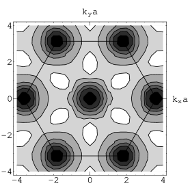
Figure 6: The lower edge of the two-spinon spectrum for the zero-flux state at $\kappa=0.3$. Axes are in dimensionless unit $k_{x,y}a$ where $a$ is lattice constant. Darker regions has lower energy. the 120 degree magnetic order arises from magnon condensation at the zone corners. See also FIG. 5.

By solving $\min\omega(\mathbf{k})=0$ together with self-consistent equations, we determined the critical quantum parameter $\kappa_{c}\approx 0.42$. We can estimate the sublattice magnetization for spin-1/2 Heisenberg model to be $58\%$ of classical spin, which probably overestimates the order since it is larger than that obtained from spin-wave theories which predicts this to be about $48\%$ Jolicoeur (1989).

IV.2 $\pi$-flux state

From FIG. 4, it is clear that there are two sites in a unit cell, distinguished by the parity of $r_{2}$. We label them by $u$ and $v$.

After Fourier transformation, the mean field Hamiltonian (7) is

$$\begin{split}H_{MF}=&\phantom{+}\sum_{\mathbf{k}}{\Psi(\mathbf{k})^{\dagger}D(\mathbf{k})\Psi(\mathbf{k})}\\ &+{N_{s}}[\mu+\mu\kappa+3J_{1}A_{1}^{2}]\end{split}$$ (27)

Here $\sum_{\mathbf{k}}$ sums over $({N_{s}}/2)$ $\mathbf{k}$-points in spinon Brillouin zone, which is one half of the hexagonal Brillouin zone of original spin model (see FIG. 5).

The vector spinon field $\Psi(\mathbf{k})$ is:

$$\Psi(\mathbf{k})=\begin{pmatrix}b_{u\mathbf{k}\uparrow}{{}^{\vphantom{\dagger}}}\cr b_{v\mathbf{k}\uparrow}{{}^{\vphantom{\dagger}}}\cr b_{u\mathbf{-k}\downarrow}^{\dagger}\cr b_{v\mathbf{-k}\downarrow}^{\dagger}\cr\end{pmatrix}$$ (28)

and the 4-by-4 matrix $D(\mathbf{k})$ has the following block form

$$\begin{pmatrix}\mu\cdot{\rm\bf 1}&-{i}P(\mathbf{k}){{}^{\vphantom{\dagger}}}\cr{i}P(\mathbf{k})^{\dagger}&\mu\cdot{\rm\bf 1}\end{pmatrix}$$ (29)

where ${\rm\bf 1}$ is the 2-by-2 identity matrix, and the 2-by-2 Hermitian matrix $P(\mathbf{k})$ can be written in terms of the Pauli matrices $\sigma^{x,y,z}$:

$$P(\mathbf{k})=J_{1}A_{1}\left[\sin(k_{1})\sigma^{z}-\sin(k_{2})\sigma^{x}-\cos(k_{3})\sigma^{y}\right]$$ (30)

This Hamiltonian can be diagonalized by a Bogoliubov transformation using a $SU(2,2)$ matrix after which we have:

$$H_{MF} = \sum_{\mathbf{k};\,a=u,v}{\omega(\mathbf{k})(\gamma_{a\mathbf{k}\uparrow}^{\dagger}\gamma_{a\mathbf{k}\uparrow}{{}^{\vphantom{\dagger}}}+\gamma_{a-\mathbf{k}\downarrow}^{\dagger}\gamma_{a-\mathbf{k}\downarrow}{{}^{\vphantom{\dagger}}}+1)}$$ (31)

$$+{N_{s}}[\mu+\mu\kappa+3J_{1}A_{1}^{2}]$$

where $\gamma$ are transformed boson operators and $a=u,v$ is a sublattice index.

The spinon dispersion is therefore four-fold degenerate with the form:

$$\omega(\mathbf{k}) = \sqrt{\mu^{2}-J_{1}^{2}A_{1}^{2}\left[\sin^{2}(k_{1})+\sin^{2}(k_{2})+\cos^{2}(k_{3})\right]}$$

Self-consistent equations comes from minimization of mean field energy (constant terms after Bogoliubov transformation).

$$6J_{1}A_{1} = -\int_{BZ}\frac{\partial\omega(\mathbf{k})}{\partial A_{1}}\mathrm{\bf d}^{2}k$$ (32)

$$1+\kappa = -\int_{BZ}\frac{\partial\omega(\mathbf{k})}{\partial\mu}\mathrm{\bf d}^{2}k$$ (33)

where the integral is over the Brillouin Zone, and $\mathrm{\bf d}^{2}k={\mathrm{d}k}_{1}{\mathrm{d}k}_{2}/(4\pi^{2})$. Recall, the amplitudes $B_{ij}$ on nearest neighbor bonds are forbidden in this state by the PSG.

On solving the self-consistent equations, the mean field energy per bond is obtained as:

$$E/\mathrm{bond}=-J_{1}A_{1}^{2}$$ (34)

and the minima of spinon dispersion are at $(k_{1},k_{2})=\pm(\pi/2,-\pi/2)$. Therefore the minima of the two-spinon spectrum are at the Brillouin zone edge-centers and center, as illustrated in FIG. 7. The distinction from the analogous diagram for the zero-flux state in FIG.  6 indicates that the $\pi$-flux state is really a distinct state from zero-flux state.

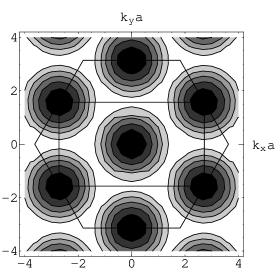
Figure 7: The lower edge of the two-spinon spectrum of the $\pi$-flux state with $\kappa=0.3$. Axes are in dimensionless unit $k_{x,y}a$ where $a$ is lattice constant. Darker regions have lower energy. Magnetic order arises from magnon condensation at the centers of the zone edges. See also FIG. 5.

The critical quantum parameter for $\pi$-flux state is found to be $\kappa_{c}\approx 0.75$. This large $\kappa_{c}$ makes the $\pi$-flux state a promising candidate of spin liquid especially given that in the zero-flux case the mean field theory seemed to overestimate magnetic order. Even in the event that magnetic order is present, it is expected to be weak, and the presence of a proximate spin liquid should be apparent at finite temperatures and energies as discussed in IsakovSenthilKim . However, for the nearest-neighbor antiferromagnet, the zero-flux state always has lower mean field energy, which is consistent with the general argument of flux-expulsion by Tchernyshyov, et. al. Tchernyshyov (2004). Later we will see that $\pi$-flux state can be stabilized as the global minimum of the mean field theory, if other terms such as next neighbor couplings or ring exchange are present in the Hamiltonian.

IV.3 Spin Configurations from Spinon Condensates

When quantum parameter $\kappa$ goes beyond its critical value the spinon dispersion becomes zero at several $\mathbf{k}$-points. Bosons condense at those $\mathbf{k}$-points, namely, the spinon field $\Psi(\mathbf{k})$ receives expectation value in ground state. We briefly analyze the structure of condensates and the corresponding spin configurations for the zero-flux state, where we follow reference Sachdev (1992), and then apply the same analysis to the $\pi$-flux state on the triangular lattice.

The zero-flux state, has spinon minima at $\mathbf{k}_{c}=(2\pi/3,2\pi/3)$. At this point, $D(\mathbf{k}_{c})$ of equation (20) has an eigenvector with zero eigenvalue

$$\Psi_{1}=\begin{pmatrix}{i},&1\end{pmatrix}^{T}$$

(^T is transposition). When $\kappa$ just exceeds $\kappa_{c}$, a condensate at $\mathbf{k}_{c}$ is obtained $\langle\Psi(\mathbf{k}_{c})\rangle=(\langle b_{\mathbf{k}_{c}\uparrow}\rangle\,\langle b_{-\mathbf{k}_{c}\downarrow}^{\dagger}\rangle)=c_{1}\Psi_{1}$. Similarly, $D(-\mathbf{k}_{c})$ has one eigenvector associated with zero eigenvalue

$$\Psi_{2}=\begin{pmatrix}-{i},&1\end{pmatrix}^{T}=\Psi_{1}^{*}$$

Condensate at $-\mathbf{k}_{c}$ is $\langle\Psi(-\mathbf{k}_{c})\rangle=c_{2}\Psi_{2}$. Here $c_{1,2}$ are two complex numbers.

The condensate on lattice site ${\mathbf{r}}$ is then given by

$$x\equiv\begin{pmatrix}\langle b_{{\mathbf{r}}\uparrow}\rangle\\ \langle b_{{\mathbf{r}}\downarrow}\rangle\end{pmatrix}=\begin{pmatrix}{i}c_{1},&-{i}c_{2}\\ c_{2}^{*},&c_{1}^{*}\end{pmatrix}\begin{pmatrix}e^{{i}\mathbf{k}_{c}\cdot{\mathbf{r}}}\\ e^{-{i}\mathbf{k}_{c}\cdot{\mathbf{r}}}\end{pmatrix}$$

and the ordered magnetic moment is $\mathbf{S}({\mathbf{r}})=(1/2)x^{\dagger}\mathbf{\sigma}x$.

This can be readily shown to give rise to the 120 degree classical Neel state, in which the classical spin is

$$\mathbf{S}({\mathbf{r}})=\mathbf{n}_{1}\cos(\mathbf{Q}\cdot{\mathbf{r}})+\mathbf{n}_{2}\sin(\mathbf{Q}\cdot{\mathbf{r}})$$ (35)

where $\mathbf{n}_{1,2}$ are orthogonal to each other and have the same length as the classical spin

$$\mathbf{n}_{1}^{2}=\mathbf{n}_{2}^{2}=\mathbf{S}^{2}$$ (36)

$\mathbf{Q}=\pm(2\pi/3,2\pi/3)$ is the wavevector of Brillouin zone corner, represented as small triangles in FIG. 5.

For $\pi$-flux state, the critical spinon wavevector occurs at $\mathbf{k}_{c}=(\pi/2,-\pi/2)$. At this point,, $D(\mathbf{k}_{c})$ of equation (29) has two eigenvectors associated with zero eigenvalue

$$\Psi_{1} = \begin{pmatrix}\frac{1-{i}}{\sqrt{3}},&-\frac{{i}}{\sqrt{3}},&0,&1\end{pmatrix}^{T}$$

$$\Psi_{2} = \begin{pmatrix}\frac{{i}}{\sqrt{3}},&-\frac{1+{i}}{\sqrt{3}},&1,&0\end{pmatrix}^{T}$$

The condensate at $\mathbf{k}_{c}$ can in general be parameterized as $\langle\Psi(\mathbf{k}_{c})\rangle=c_{1}\Psi_{1}+c_{2}\Psi_{2}$. Similarly, $D(-\mathbf{k}_{c})$ has two eigenvectors associated with zero eigenvalue

$$\Psi_{3} = \begin{pmatrix}\frac{1+{i}}{\sqrt{3}},&\frac{{i}}{\sqrt{3}},&0,&1\end{pmatrix}^{T}=\Psi_{1}^{*}$$

$$\Psi_{4} = \begin{pmatrix}-\frac{{i}}{\sqrt{3}},&-\frac{1-{i}}{\sqrt{3}},&1,&0\end{pmatrix}^{T}=\Psi_{2}^{*}$$

and the condensate at $-\mathbf{k}_{c}$ is parameterized as: $\langle\Psi(-\mathbf{k}_{c})\rangle=c_{3}\Psi_{3}+c_{4}\Psi_{4}$. Here $c_{1,2,3,4}$ are four complex numbers.

Returning to real space, the spinon condensate on sublattice $u$ is

$$\begin{split}x_{u}\equiv&\begin{pmatrix}\langle b_{u{\mathbf{r}}\uparrow}\rangle\\ \langle b_{u{\mathbf{r}}\downarrow}\rangle\end{pmatrix}\\ =&\begin{pmatrix}\frac{1-{i}}{\sqrt{3}}c_{1}+\frac{{i}}{\sqrt{3}}c_{2},&\frac{1+{i}}{\sqrt{3}}c_{3}-\frac{{i}}{\sqrt{3}}c_{4}\\ c_{4}^{*},&c_{2}^{*}\end{pmatrix}\begin{pmatrix}e^{{i}\mathbf{k}_{c}\cdot{\mathbf{r}}}\\ e^{-{i}\mathbf{k}_{c}\cdot{\mathbf{r}}}\end{pmatrix}\end{split}$$

while the spinon condensate on sublattice $v$ is

$$\begin{split}x_{v}\equiv&\begin{pmatrix}\langle b_{v{\mathbf{r}}\uparrow}\rangle\\ \langle b_{v{\mathbf{r}}\downarrow}\rangle\end{pmatrix}\\ =&\begin{pmatrix}-\frac{{i}}{\sqrt{3}}c_{1}-\frac{1+{i}}{\sqrt{3}}c_{2},&\frac{{i}}{\sqrt{3}}c_{3}-\frac{1-{i}}{\sqrt{3}}c_{4}\\ c_{3}^{*},&c_{1}^{*}\end{pmatrix}\begin{pmatrix}e^{{i}\mathbf{k}_{c}\cdot{\mathbf{r}}}\\ e^{-{i}\mathbf{k}_{c}\cdot{\mathbf{r}}}\end{pmatrix}\end{split}$$

The ordered magnetic moment on sublattice $p$ is $(1/2)\left(x_{p}\right)^{\dagger}\mathbf{\sigma}x_{p}$ for $p=u,v$ respectively and is present at wavevectors at the mid points of the Brillouin Zone edges shown via black hexagons in FIG. 5.

Under the constraint that the magnitude of condensate is uniform (which is required to have uniform magnitude for the ordered moments ), we find a continuum of four-sublattices ordered states, which is consistent with previous classical energy analysis on triangular lattice magnets with interactions that favor order at these wavevectors Korshunov (1993). The classical spin in the four-sublattices states is

$$\mathbf{S}({\mathbf{r}})=\mathbf{n}_{1}(-1)^{r_{1}}+\mathbf{n}_{2}(-1)^{r_{2}}+\mathbf{n}_{3}(-1)^{r_{1}+r_{2}}$$ (37)

where $\mathbf{n}_{1,2,3}$ are three vectors orthogonal to each other, and

$$\mathbf{n}_{1}^{2}+\mathbf{n}_{2}^{2}+\mathbf{n}_{3}^{2}=\mathbf{S}^{2}.$$ (38)

Generally speaking this configuration is non-coplanar if $|\mathbf{n}_{1,2,3}|$ are all nonzero. However, previous analysis confirmed the existence of ”order from disorder”phenomena, namely, quantum or thermal fluctuation will lift the accidental degeneracy and favor a collinear state in large S models with next nearest neighbor antiferromagnetic exchange Jolicoeur (1990); Chubukov (1992), which corresponds to the case that only one of $\mathbf{n}_{1,2,3}$ is nonzero.

It has been argued that ring exchange will favor a non-coplanar stateKorshunov (1993). The classical ground state will then be a tetrahedral configuration with equal angle between any two of the four spins. In the above expression, this state is realized when $\mathbf{n}_{1,2,3}$ have same magnitude.

However, on studying the ordered state with weak spinon condensation, the constraint that the magnitude of the spinon condensate is uniform enforces the additional condition on the $\mathbf{n}_{1,2,3}$, that one of the following three equations must be satisfied

$$|\mathbf{n}_{1}| = |\mathbf{n}_{2}|+|\mathbf{n}_{3}|$$ (39a)

$${\rm or}\,\,\,|\mathbf{n}_{2}| = |\mathbf{n}_{3}|+|\mathbf{n}_{1}|$$ (39b)

$${\rm or}\,\,\,|\mathbf{n}_{3}| = |\mathbf{n}_{1}|+|\mathbf{n}_{2}|$$ (39c)

Thus the classical degeneracy is not entirely lifted at this level. Also, neither the collinear state nor the tetrahedral state can be obtained from weak spinon condensates from this spin liquid state - although the wavevectors of all these ordered states are identical. This implies that if there is a continuous phase transition out of the $\pi$-flux spin liquid phase, the proximate spin ordered state is not the collinear or tetrahedral state, but these are realized via further phase transitions on increasing the size of the spin. We are still seeking a simple explanation for these results.

V Hamiltonians Stabilizing the $\pi$-flux State

The $\pi$-flux spin liquid state differs in several respects from the zero-flux state; also, its stability against magnetic ordering up to a relatively large quantum parameter $\kappa_{c}=0.75$ (in a nearest neighbor model) suggests its physics may be important for understanding physical spin-1/2 models. Hence it is of interest to ask what interactions might stabilize such a $\pi$-flux state.

A clue is provided by the fact that the lowest energy triplet excitations of such a state are located at the midpoints of the Brillouin zone edges. This is precisely the ordering wave-vector for classical spins on the triangular lattice in a model with next-nearest-neighbour ($J_{2}$) antiferromagnetic interactions in addition to nearest-neighbour antiferromagnetic interactions ($J_{1}$) in the range $0.125J_{1}<J_{2}<J_{1}$Jolicoeur (1990). It is conceivable that on reducing the size of the spin in this model from infinity (the classical limit) to S=1/2, the system enters a spin liquid state described by the $\pi$-flux state, although strictly the quantum parameter for this case is $\kappa=1$.

A second possibility arises from ring exchange - it is well known that there are several realization of S=1/2 quantum antiferromagnets on the triangular lattice where ring exchange plays an important role. These include monolayers of ³He adsorbed on graphite Masutomi (2004), and the organic quantum antiferromagnet $\kappa$-(ET)₂ Cu₂(CN)₃ Kanoda (2003). Also, exact diagonalization studies of the triangular lattice S=1/2 magnet with ring exchange has uncovered unusual properties Misguich (1999). In a recent variational study with fermionic mean field states by Motrunich Motrunich (2004) it was found that ring exchange of the sign that arises naturally with electrons, favors a state with zero flux. Here we will investigate the effect of ring exchange on the Schwinger boson states - in particular for which sign of the exchange one might favor the $\pi$-flux state. We find that including four spin ring exchange with the sign as obtained from the Hubbard model stabilizes the $\pi$-flux state.

Here we give some physical arguments as to why next-neighbor antiferromagnetic interactions and the ring term will stabilize $\pi$-flux state over the zero-flux state.

V.1 Effect of Next Neighbour Interactions $J_{2}$:

For zero-flux state, nearest-neighbor amplitudes $B_{1}$ and $A_{1}$, and next-nearest-neighbor amplitudes $B_{2}$ are nonzero, while the next-nearest-neighbor amplitude $A_{2}$ is zero. Note that $B_{2}$ is nonzero even if next-nearest-neighbor coupling $J_{2}$ is zero.

$$\begin{split}\frac{E^{[\mathrm{zero-flux}]}}{\mathrm{bond}\cdot J_{1}}=&\phantom{+}\left(B^{[\mathrm{zero-flux}]}_{1}\right)^{2}-\left(A^{[\mathrm{zero-flux}]}_{1}\right)^{2}\\ &+\frac{J_{2}}{J_{1}}\left(B^{[\mathrm{zero-flux}]}_{2}\right)^{2}\end{split}$$

In contrast, for the $\pi$-flux state, $A_{1}$ and $A_{2}$ are nonzero, while $B_{1}$ and $B_{2}$ are zero. Note, $A_{2}$ is nonzero even if $J_{2}$ is zero.

$$\frac{E^{[\pi\mathrm{-flux}]}}{\mathrm{bond}\cdot J_{1}}=-\left(A_{1}^{[\pi\mathrm{-flux}]}\right)^{2}-\frac{J_{2}}{J_{1}}\left(A_{2}^{[\pi\mathrm{-flux}]}\right)^{2}$$

It is readily shown with the self consistent values of the mean field amplitudes that for $J_{2}=0$, $E^{[\mathrm{zero-flux}]}<E^{[\pi\mathrm{-flux}]}$, i.e. the zero-flux state is preferred at the mean field level. However, if we increase $J_{2}$ from zero, we do not expect the ansatz to change rapidly, thus the energy for zero-flux state will have a positive slope with respect to $J_{2}$, while the $\pi$-flux state has a negative slope. We may then expect a first-order transition between the two states. This is consistent with previous analysis of $J_{1}-J_{2}$ model in the opposite limit of semiclassical spins, where a transition between the 120 degree state (the magnetically ordered analog of the zero-flux state and the colinear state, the magnetically ordered analog of the $\pi$-flux state is found on increasing $J_{2}$ Chubukov (1992); Deutscher (1993). From the classical energy analysisJolicoeur (1990), we know that in large-$S$ limit $\alpha=1/8$ is the critical point between different ordered states with ordering wavevectors at the BZ corners vs. BZ edge midpoints. Thus one might expect that a moderate next-nearest-neighbor term ($1/8<\alpha<1$) will stabilize the $\pi$-flux state over the zero-flux state in the quantum limit, since these states have short range order (two spinon minima) at precisely these wavevectors. We now provide estimates for the phase boundary (the critical ratio $\alpha=J_{2}/J_{1}$) between the zero-flux and $\pi$-flux spin liquid phases as a function of the quantum parameter $\kappa$.

Small $\kappa$ analysis: The competition between different spin liquid states can be studied analytically in the limit of small-$\kappa$Tchernyshyov (2004). In this case the magnitude of the ansatz $A_{ij}$ and $B_{ij}$ are small. Then, we can develop a series expansion of the self-consistent equations in $\kappa$, and find solutions.

First, we use this expansion to look at the $J_{1}$-$J_{2}$ model, with $\alpha\equiv J_{2}/J_{1}<1$ and sufficiently small quantum parameter $\kappa$.

The energy difference between the zero-flux and the $\pi$-flux state in this limit is:

$$\frac{E^{[\mathrm{zero-flux}]}-E^{[\pi\mathrm{-flux}]}}{\mathrm{bond}\cdot J_{1}} = -(1-\alpha)\left[\frac{\kappa}{6}\right]^{2}+\frac{2\alpha}{1-\alpha}\left[\frac{\kappa}{6}\right]^{3}$$ (40)

$$+\left(\frac{87}{4}+23\alpha+72\alpha^{2}\right)\left[\frac{\kappa}{6}\right]^{3}$$

$$+O(\kappa^{4})$$

From the above expressions for mean field energy difference, we can find the transition point between the zero-flux and $\pi$-flux states to lowest order in $\kappa$.

$$\alpha_{c}=1-\sqrt{\kappa/3}$$ (41)

In the limit of vanishing $\kappa$ the zero-flux state is preferred until the next-neighbor bond is stronger than the nearest neighbor bond. However, this critical ratio decreases rapidly with increasing $\kappa$.

In the small $\kappa$ limit one can ignore the spin carrying excitations. Then, going beyond the mean field theory the relevant degrees of freedom are the gauge excitations, which in this case correspond to those of an Ising gauge theory. The distinction between zero and $\pi$-flux states in this limit we believe has to do with the the sign of plaquette energy term that penalizes Ising vortex excitations in the case of the zero-flux state, but prefers a ground state with a uniform background ”flux”of such vortices in the case of the $\pi$-flux state.

Numerical Solution: The mean field equations can be numerically solved to obtain the competition between the zero-flux and $\pi$-flux states and states with magnetic order. This is shown in FIG. 8. The critical value $\kappa_{c}^{[\pi\mathrm{-flux}]}$ at which spinon condensation occurs for the $\pi$-flux state is shown by the dashed and solid red line. If the $\pi$-flux state is stabilized, then above this line spinon condensation leads to magnetic order at the B.Z. edge centers (M-points). There are a number of distinct ordering patters consistent with this ordering wavevector - which makes an analysis of the ordered phase a delicate one; and we do not attempt it here. Therefore, the phase diagram shown in FIG. 8 is strictly speaking only to be trusted below this $\kappa_{c}^{[\pi\mathrm{-flux}]}$ line(red line). However, certain extrapolations above this line can be made with some degree of confidence.

The first-order phase boundary between the $\pi$-flux and zero-flux spin liquid states is shown by the black line in FIG. 8. At small $\kappa$ it approaches $\alpha=1$ via the analytic form derived previously 41. It intersects the spinon condensation line for the $\pi$-flux state at $\alpha=0.46,\ \kappa=0.47$.

The zero-flux state is stabilized at smaller values of $\alpha$, and sufficiently small quantum parameter $\kappa<\kappa_{c}^{[\mathrm{zero-flux}]}$, where the critical quantum parameter for spinon condensation in this state is shown by the blue line. Spinon condensation is expected to lead to the 120 degree state on crossing this lineincommensurate . Again, this is most reliably established if the ordered states with wavevectors at the M-points (M-states) are not in the picture, which is the case below the dashed red line in FIG. 8. An interesting aspect of the phase diagram is the large values of $\kappa_{c}^{[\mathrm{zero-flux}]}\approx 1.8$ that arise, if the M-states are neglected. This is believed to be a result of frustration of the 120 degree Neel order by next neighbor interactions. While some part of this spin liquid region in the phase diagram above $\kappa_{c}^{[\pi\mathrm{-flux}]}$ might be occupied eventually by magnetically ordered M-states, the existence of zero-flux spin liquid states for fairly large values of the quantum parameter is likely to persist, making the $J_{1}$-$J_{2}$ model an interesting candidate for spin liquid physics that deserves further attention.

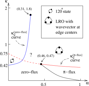
Figure 8: (color online) The mean field phase diagram of the triangular lattice antiferromagnet with nearest neighbor $J_{1}$ and next-neighbor $J_{2}$ interactions, as a function of the ratio $\alpha=J_{2}/J_{1}$ and quantum parameter $\kappa$. The diagram is a quantitatively reliable solution of mean field equations in the region near to and below the red line (dashed and solid) where spinon condensation of the $\pi$-flux state occurs. Just above the solid red line, magnetic ordering at the Brillouin zone M-point occurs, while below it the $\pi$-flux spin liquid phase is obtained. The black line is the first-order phase boundary between the zero-flux and $\pi$-flux spin liquid phases, while the blue line represents the onset of 120 degree magnetic order. The quick rise of this line to large values of $\kappa$ is due to frustration of the 120 degree Neel order by next neighbor interactions. If uninterrupted by magnetic order (of the M type) this may open a window of spin liquid for physical spin values in this model.

V.2 Effect of Ring Exchange

In addition to the exchange interaction between a pair of spins, multi-spin interactions are also present in insulators with non-negligible charge fluctuations. While for spin one-half systems, the three spin interaction can be expressed in terms of two spin exchange, a new term is generated when considering four spin interactions. The four spin ring exchange term is:

$$H_{Ring} = J_{Ring}\sum{(P_{4}+h.c.)}$$ (42)

$$P_{4} = b_{i\delta}^{\dagger}b_{i\alpha}{{}^{\vphantom{\dagger}}}b_{j\alpha}^{\dagger}b_{j\beta}{{}^{\vphantom{\dagger}}}b_{k\beta}^{\dagger}b_{k\gamma}{{}^{\vphantom{\dagger}}}b_{l\gamma}^{\dagger}b_{l\delta}{{}^{\vphantom{\dagger}}}$$ (43)

where $P_{4}$ is the four spin permutation operator, which is written out conveniently in terms of the Schwinger boson operators as above. The sites $i,j,k,l$ form a rhombus and $\alpha,\,\beta,\,\gamma,\,\delta\in\{\uparrow,\,\downarrow\}$ are spin indices. The above bosonic spinon representation of the ring-exchange may be checked by expanding it in terms of the spin operators in the spin-1/2 case and verifying it has the required form Spin . A more efficient way to prove this identity will be to establish a correspondence with the fermionic spinon representation of ring exchange which is done later in this section.

From the $t/U$ expansion of the Hubbard model MacDonald (1988), it is found that $J_{Ring}=20t^{4}/U^{3}$ and is positive. In the following, when we consider ring exchange term we neglect the next-nearest-neighbor term, and vise versa. Evaluating the ring exchange term in the mean field ground state, one find that the result contains:

$$\langle H_{Ring}\rangle_{MF}=8J_{Ring}(A_{ij}{{}^{\vphantom{\dagger}}}A_{jk}^{*}A_{kl}{{}^{\vphantom{\dagger}}}A_{li}^{*}+c.c)+\ldots$$ (44)

which is the term we used to define flux. The other terms are small, especially in the small-$\kappa$ regime. This term clearly has different signs for zero-flux and $\pi$-flux states, and favors the $\pi$-flux states when $J_{Ring}$ is positive. Thus we also expect a possible transition from zero-flux state to $\pi$-flux state when we tune ring exchange coupling.

It is well known that the ring exchange term, derived from the Hubbard model, has positive (negative) coupling constant when expressed in terms of a permutation operator, if the loop length is even (odd)Thouless (1965). This can be seen as follows. Since the ring exchange term arises from virtual electron hopping process lowering the energy, the effective term generated is $-K_{L}[c_{1\sigma_{L}}^{\dagger}c_{L\sigma_{L}}{{}^{\vphantom{\dagger}}}c_{L\sigma_{L-1}}^{\dagger}c_{L-1\sigma_{L-1}}{{}^{\vphantom{\dagger}}}\cdots c_{2\sigma_{1}}^{\dagger}c_{1\sigma_{1}}{{}^{\vphantom{\dagger}}}+\mathrm{h.c.}]$ where $c_{i\sigma}$ are electron annihilation operators with site index $i$ and spin index $\sigma$, and $K_{L}>0$. Clearly this term includes a permutation operator for length $L$ loop $(-1)^{L-1}(-K_{L})c_{1\sigma_{L}}^{\dagger}c_{1\sigma_{1}}{{}^{\vphantom{\dagger}}}c_{2\sigma_{1}}^{\dagger}c_{2\sigma{2}}{{}^{\vphantom{\dagger}}}\cdots c_{L\sigma_{L-1}}^{\dagger}c_{L\sigma_{L}}{{}^{\vphantom{\dagger}}}+\mathrm{h.c.}$. So for $L$ even we have $+K_{L}(P_{L}+\mathrm{h.c.})$.

While the above discussion has been phrased in terms of fermionic spinons, we can now translate those observations into the bosonic spinon language. It turns out that the permutation operator has the same form and sign in terms of both fermion (electron) operators and Schwinger boson operators. We give two arguments in support of this below. First, notice that spin $1/2$ operators has the same representation in Schwinger boson and ”Schwinger fermion”(electrons) scheme. Assume that spin indices $\alpha,\ \beta$ take values of +1(spin up) and -1(spin down). For $S=1/2$ system we have $c_{i\alpha}^{\dagger}c_{i\beta}{{}^{\vphantom{\dagger}}}=(2S+2\alpha S^{z})\delta_{\alpha,\beta}+\left[(1+\alpha)S^{+}+(1-\alpha)S^{-}\right]\delta_{\alpha,-\beta}=b_{i\alpha}^{\dagger}b_{i\beta}$. Therefore we can simply replace fermion operator $c$ by Schwinger boson operator $b$ in the permutation operator. The second argument is to use Jordan-Wigner transformation to change electronic operators into boson. After replacing fermionic operators with bosons the Jordan-Wigner string operators becomes a constant under the constraint of constant($2S$) particles on each site.

Now we evaluate the above ring exchange operator for longer length loops in the Schwinger boson mean field states. We focus on even length loops since we expect the dominant amplitudes to be given by the $A_{ij}$s, which can only give rise to even length loops if they are the only amplitudes that count. The dominant term is $2\cdot 2^{L/2}\cdot(A_{1,2}{{}^{\vphantom{\dagger}}}A_{2,3}^{*}\cdots A_{L-1,L}{{}^{\vphantom{\dagger}}}A_{L,1}^{*}+\mathrm{h.c.})$. This is not exactly the term defining flux in the loopTchernyshyov (2004), which has an additional minus sign for each $A^{*}$. Namely the result is $2\cdot 2^{L/2}\cdot(-1)^{L/2}(\mathrm{term\ defining\ flux+h.c.})$. It is then clear that for $L=4,8,12,\dots$ the ring exchange term favors $\pi$-flux in the loop, while for $L=6,10,14,\dots$ it favors zero flux. It is amusing to contrast this with the result for mean field theories based on a fermionic spin representation, where ring exchange favors states with zero-flux Motrunich (2004). The difference has to do with the different definitions for flux that naturally appear in these two theories.

Small $\kappa$ Analysis: As argued previously, raising the value of $J_{Ring}/J_{1}$ above a critical value, favors the $\pi$ flux state over the zero-flux state. We now study the effect of ring exchange term by evaluating it in the zero-flux and $\pi$-flux states, in the limit of small $\kappa$ where an analytic solution may be obtained. Another benefit for going to small-$\kappa$ limit is that larger-ring exchange effect (e.g. length-six ring) is controlled by small parameter $\kappa$ as $\kappa^{\mathrm{length/2}}$ according to Tchernyshov, et. al. Tchernyshyov (2004), therefore only the energetics of length-four ring, namely the rhombus, is important.

The procedure described above is of course only the lowest order term, but we expect it to give us the correct qualitative behavior. For zero-flux state, the contribution from the ring exchange term is $(\kappa^{2}/6)J_{Ring}$ per rhombus to lowest order. For $\pi$-flux state, it is $-(\kappa^{2}/18)J_{Ring}$ per rhombus to lowest order. Therefore, a positive $J_{Ring}$ clearly favors the $\pi$-flux state. Since for every site, there are three bonds and three rhombi on average, we can find the transition point in the $\kappa\rightarrow 0$ limit to be :

$$[J_{Ring}/J_{1}]_{c}=1/8.$$ (45)

Several other theories predict a transition for the triangular lattice antiferromagnet while tuning this ratio $J_{Ring}/J_{1}$, although the phases appearing may be different. Motrunich’s fermionic variational method Motrunich (2004) predicts a transition from a ”$\pi$-flux”fermionic mean field state to ”zero-flux”mean field state when $J_{Ring}/J_{1}$ increases over about $0.35$. A previous bosonic mean field phase diagram Misguich (1998) predict a transition from 120 degree Neel-ordered state to collinear-ordered state when this ratio increases over $1/3$. It is interesting that we found a similar transition between two disordered spin liquid state for sufficiently small $\kappa$, with short ranged order at precisely these two wavevectors, as this ratio is increased.

Numerical Solution: For finite $\kappa$, the numerical solution of the mean field equations have been obtained for the nearest-neighbor model below the critical value $\kappa_{c}$ for both states. We can make a lowest order perturbative treatment of next-nearest-neighbor and ring exchange terms, namely we evaluate these two terms in the mean field ground state of nearest-neighbor model and thus obtain the transition point. We found approximate critical value of $\alpha\equiv J_{2}/J_{1}$ and $J_{Ring}/J_{1}$, listed in TABLE 1.

$\kappa$	$J_{Ring}/J_{1}$
0.05	0.126
0.10	0.127
0.20	0.128
0.30	0.129

Table 1: Approximate finite $\kappa$ result for critical $J_{Ring}/J_{1}$ at which the zero-flux state gives way to the $\pi$-flux state on the triangular lattice.

VI Spin Liquid States on the Kagomé Lattice

The Kagomé lattice has three sites in one unit cell, labeled by $u,\ v,\ w$ (see FIG. 9).

Figure 9: Coordinates system of Kagome lattice. Rhombus enclosed by dash lines is the unit cell at origin. Three sites with black dots form the basis of lattice. Black rhombus is an example of length-eight loops.

We label a unit cell by ${\mathbf{r}}=(r_{1},r_{2})$ and label a site by $(r_{1},r_{2})_{p}$ where $p=u,v,w$.

VI.1 Projective Symmetry Group Analysis of the Kagomé Lattice

We would like to obtain the possible symmetric spin liquid states on the Kagomé lattice described within the Schwinger boson approach. Again, a Projective Symmetry Group analysis will be carried out just as was done on the triangular lattice. A gauge transformation ${G}$ is then described by three phase functions ${\phi_{u}}({\mathbf{r}}),{\phi_{v}}({\mathbf{r}}),{\phi_{w}}({\mathbf{r}})$.

For simplicity we will consider ansatz with $A_{ij}=\frac{1}{2}\epsilon_{\sigma\sigma^{\prime}}\langle b_{i\sigma}b_{j\sigma^{\prime}}\rangle$ only. These amplitudes are naturally present for predominantly anti-ferromagnetic interactions, and can be strictly justified in large-N limit Sachdev (1992). Then, due to the frustrated nature of the Kagomé lattice, the Invariant Gauge Group is $Z_{2}$, generated by

$${\phi_{u}}({\mathbf{r}})={\phi_{v}}({\mathbf{r}})={\phi_{w}}({\mathbf{r}})=\pi$$

thus we will study $Z_{2}$ spin liquid states within the Schwinger boson approach.

In the above coordinates system the space group is generated by two translations ${T_{1}},\ {T_{2}}$, reflection ${\sigma}$ and 60 degree rotation ${R_{\frac{\pi}{3}}}$. The first two generators preserve sublattices. The reflection exchanges $u$ and $v$ sublattices. The rotation is a cyclic permutation of three sublattices $u\rightarrow v,\ v\rightarrow w,\ w\rightarrow u$.

For each space group generator $X$ we can associate a gauge transformation described by three phase functions ${\phi_{X,u}}({\mathbf{r}}),{\phi_{X,v}}({\mathbf{r}}),{\phi_{X,w}}({\mathbf{r}})$.

The procedure of solving the for the different PSGs allowed by the algebraic constraints imposed by relations between symmetry elements is parallel to triangular case, except that one has to keep track of the index of sublattices. It turns out that the three phase functions can be chosen to be identical. The solution of algebraic PSG (details in Appendix C) is then identical to the triangular lattice case except that the phase functions have one more index.

$${\phi_{{T_{1}},p}}(r_{1},\ r_{2}) = 0$$ (46a)

$${\phi_{{T_{2}},p}}(r_{1},\ r_{2}) = p_{1}\pi r_{1}$$ (46b)

$${\phi_{{\sigma},p}}(r_{1},\ r_{2}) = p_{2}\pi/2+p_{1}\pi r_{1}r_{2}$$ (46c)

$$2{\phi_{{R_{\frac{\pi}{3}}},p}}(r_{1},\ r_{2}) = p_{3}\pi+p_{1}\pi r_{2}(r_{2}\!-\!1\!+\!2r_{1})$$ (46d)

where $p=u,v,w$. Thus, in the case of the Kagomé lattice too, there are not more than 8 symmetric $Z_{2}$ spin liquid states, corresponding to the two values that each of the $p_{1},\,p_{2},\,p_{3}$ can take on.

If we now specialize to states that have non-vanishing nearest-neighbor amplitudes $A_{ij}$, we have more realizations of the algebraic PSG. The only additional restriction(c.f. SEC. III.2) is that bond $(0,0)_{u}\rightarrow(0,0)_{w}$ can be related to bond $(0,0)_{v}\rightarrow(0,0)_{w}$ by both reflection and 60 degree rotation. This gives one constraint $p_{2}=1-p_{3}$. In all these ansatz the amplitudes $A_{ij}$ are real and of uniform magnitude.

VI.2 Spin Liquid States on the Kagomé

The four realizations are listed below. We will use the same convention of $\mathbf{k}$-space coordinates system as triangular case by taking the lattice constant as unity (the length of nearest-neighbor bond is 1/2). It is convenient to divide the four states into two pairs, two with $p_{1}=0$ and two with $p_{1}=1$. The first condition implies that the generators of translation commute, the analog of the zero-flux state, while the second condition implies a flux of $\pi$ in a unit cell. It will turn out that the two zero-flux states correspond to the two states discussed earlier by Sachdev in the context of the Kagomé lattice, while the two $pi$-flux states have not previously been discussed.

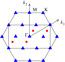
Figure 10: (Color online). $\mathbf{k}$-space of Kagomé lattice. The large hexagon is Brillouin zone of original Kagomé lattice and the two $p_{1}=0$ ansatz. The large rectangle is Brillouin zone of the two $p_{1}=1$ ansatz, which enclose a flux of $\pi$ in their unit cells. Red dots are the minima of the spinon dispersion for both $p_{1}=1$ states within the reduced Brillouin zone. Blue triangles are the locations of the minima of the lower edge of the two-spinon spectrum for both $p_{1}=1$ states.

The Zero-Flux States:

1. The first state we consider is characterised by $p_{1}=0,\ p_{2}=0,p_{3}=1$. This is the large-N ground state identified by Sachdev for the nearest neighbor antiferromagnet, which he called $Q_{1}=-Q_{2}$ stateSachdev (1992).

This state has zero-flux in both length-six hexagon and length-eight rhombus, hence we will also refer to it as [$0$Hex,$0$Rhom]. Its critical quantum parameter $\kappa_{c}\approx 0.54$. The spinon dispersion has minima at corners of Brillouin zone $\mathbf{k}=\pm(2\pi/3,2\pi/3)$, and so does the two-spinon spectrum. After spinon condensation it gives rise to the $\sqrt{3}\times\sqrt{3}$ magnetically ordered classical ground state.

2. The second state we consider is characterized by $p_{1}=0,\ p_{2}=1,p_{3}=0$. This is another state considered by Sachdev and was called the $Q_{1}=Q_{2}$ stateSachdev (1992).

This state has $\pi$ flux in length-six hexagon and zero-flux in length-eight rhombus, hence we will also refer to it as [$\pi$Hex,$0$Rhom]. Its critical quantum parameter $\kappa_{c}\approx 0.50$. The spinon dispersion has minima at centers of Brillouin zone $\mathbf{k}=(0,0)$, so does the two-spinon spectrum. After spinon condensation it gives rise to the translational invariant classical ground state.

The $\pi$-Flux States:

3. The third state we consider is characterized by $p_{1}=1,\ p_{2}=0,p_{3}=1$. The ansatz is given in FIG. 19 in the Appendix C and has not been considered before. Due to the presence of flux in the unit cell, a doubled the unit cell needs to be considered for the spinons.

This state has $\pi$ flux in both length-six hexagon and length-eight rhombus, hence we will also refer to it as [$\pi$Hex,$\pi$Rhom]. Thus, in anearest neighbor model it is expected to have the highest energy of the four states for same $\kappa$ in the small $\kappa$ regime.

Its critical quantum parameter is fairly large, $\kappa_{c}\approx 0.93$. The minima of spinon dispersion is at $\mathbf{k}=\pm(\pi/6+n\pi,\pi/6+m\pi)$, where $n,\ m$ are integers(see FIG. 10). Thus the two-spinons spectrum lower edge has minima at $\pm(\pi/3+n\pi,\pi/3+m\pi)$ and $(n\pi,m\pi)$. In addition to the Brillouin zone center, corners and edge centers, minima are also present at the halfway points to the corners.

Figure 11: Ansatz of the $p_{1}=1,\ p_{2}=1,\ p_{3}=0$ state. Presence of $\pi$ flux in the Kagome lattice unit cell leads to unit cell doubling, which is now defined by the dashed rhombus. Six sites with black dots form the basis. All nearest-neighbor $A_{ij}$ are real and of the same magnitude, and are positive in the directions shown. This spin liquid ansatz has zero flux in the length six hexagonal loops but $\pi$ flux in the length eight loops such as the rhombus, hence [$0$Hex,$\pi$Rhom]. It has a large critical quantum parameter $\kappa_{c}=2.0$.

4. The last state we consider is $p_{1}=1,\ p_{2}=1,p_{3}=0$. The ansatz is given in FIG. 11 and has not been considered before.

This state has zero flux in length-six hexagon and $\pi$ flux in length-eight rhombus,hence we will also refer to it as [$0$Hex,$\pi$Rhom] .

It is potentially the most interesting of the states considered so far since its critical quantum parameter $\kappa_{c}\approx 2.0$ is greater than unity. This means that this state is very likely to be a symmetric spin liquid state for spin-1/2 system if it can be realized. The large value of $\kappa_{c}$ is a result of the dispersion of the relevant spinon bands being nearly flat along certain directions in the Brillouin zone.

However, since this state has $\pi$ flux in the length-eight rhombus, it is, by the general argument of flux-expulsion by Tchernyshyov et. al.Tchernyshyov (2004) expected to have a higher mean field energy than Sachdev’s ground state if we consider a pure nearest-neighbor Heisenberg model. In the small $\kappa$ limit the energy difference will be the order of $\kappa^{4}$. However, it must also be kept in mind that mean field energetics is not precisely the same as the true energetics of the system.

Given the interesting nature of this state we can ask what interactions are likely to stabilize it within mean field theory, relative to the Sachdev ground state. From our previous analysis of ring exchange we know that adding ring exchange interactions of the sign obtained from the Hubbard model favors zero flux in loops of length six and $\pi$ flux in loops of length eight. This is precisely satisfied by loops in this ansatz as can be checked from the FIG. 11. Therefore the Kagomé antiferromagnet with ring exchange may be a good system to realize a spin liquid phase.

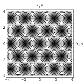
Figure 12: Two-spinons spectrum lower edge of the $p_{1}=1,\ p_{2}=0,\ p_{3}=1$ state at $\kappa=\kappa_{c}=0.9$. Axes are in dimensionless unit $k_{x,y}a$ where $a$ is lattice constant(two times nearest neighbor distance). Darker regions have lower energy.

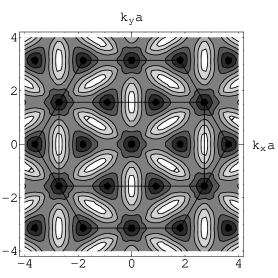
Figure 13: Two-spinons spectrum lower edge of the $p_{1}=1,\ p_{2}=1,\ p_{3}=0$ state at $\kappa=\kappa_{c}=2.0$. Axes are in dimensionless unit $k_{x,y}a$ where $a$ is lattice constant(two times nearest neighbor distance). Darker regions have lower energy. Although the two spinon minima occur at the same wavevector locations as in the previous $p_{1}=1,\ p_{2}=0,\ p_{3}=1$ state, the differences in the dispersion are apparent.

The position of minima of spinon dispersion and two-spinons spectrum lower edge are the same as in the previous state: $p_{1}=1,\ p_{2}=0,p_{3}=1$. However, the spinon dispersions of these two states are not identical. In particular the present $p_{1}=1,\ p_{2}=1,p_{3}=0$ state has three doubly-degenerate dispersion branches while previously discussed the $p_{1}=1,\ p_{2}=0,p_{3}=1$ state has six non-degenerate dispersion branches. Other differences between these two states may be observed in the contour plots of the lower edge of the two spinon dispersions in FIG. 13 and FIG. 12 respectively. A variety of magnetically ordered states can arise from spinon condensation in both these cases; the magnetic states so obtained and the associated quantum transitions would be an interesting topic for future study.

VII Conclusions

We have extended the projective symmetry group analysis, previously used to classify fermionic mean field states, to bosonic mean field states of quantum antiferromagnets on the triangular and Kagomé lattices. This allowed us to access fundamentally different spin liquid states and ensure that potentially interesting states were not overlooked. On the triangular lattice a new $Z_{2}$ symmetric spin liquid state ($\pi$-flux state) emerged from this analysis and was studied. This state is distinct from the previously studied bosonic mean field state (zero-flux or Sachdev state), which can be seen in that they have different spinon and two-spinons dispersions . The nature of the ordered state resulting from spinon condensation turns out to be more intricate in this case, as is the quantum ordering transition, and is a topic for further study. Although this state is less favorable from the point of view of mean field energy as compared to the zero-flux state in the case of nearest neighbor interactions, it is stabilized by the inclusion of moderate next nearest-neighbor or ring exchange interactions with signs as derived from the Hubbard model. The mean field analysis suggests that the triangular lattice model with next neighbor antiferromagnetic interactions might be favorable for realizing spin liquid ground states.

We have also studied $Z_{2}$ symmetric spin liquid states on the Kagomé lattice using the PSG technique. Again we find only a few candidate states, in particular two physically interesting states are found which are analogous to the $\pi$-flux state on the triangular lattice. In particular, one of these states has a remarkably large value for the critical quantum parameter $\kappa_{c}=2.0$ which implies that if realized, it would be stable against magnetic order for physical values of the spin. We find that ring exchange interactions would stabilize precisely this state, making the Kagomé model with ring exchange an attractive model to study in the search for spin liquid phases. Stability of these states to other forms of order, such as valence bond solid order, is important to understand but were not addressed in the present work. Also, the relation between fermionic mean field states, classified via the $SU(2)$ PSGs and the bosonic spinon mean field theories studied in this paper with their $U(1)$ PSGs remains unclear and is a topic for future study.

VIII Acknowledgements

We would like to thank O. Motrunich and C. Nayak for discussions. A.V. was supported by A. P. Sloan Foundation Fellowship and by DOE LDRD DEA 3664LV.

Appendix A Solution to algebraic PSGs of Triangular Lattice

In this appendix we derive the allowed PSGs for symmetry spin liquids on the triangular lattice characterized by a $Z_{2}$ gauge group. Essentially, we need to make sure that the constraints imposed by various identities between symmetry group elements are satisfied by the PSG. In particular the ansatz must satisfy the relations in equations (16a to 16h). It turns out that if a PSG satisfies all these constraints, then other relations between symmetry group elements are automatically satisfied. This is because any group element written as a string containing products of generators can be brought into a ”normal ordered”form using just these operations where normal ordering implies a form of the kind: ${\sigma}^{s}[{R_{\frac{\pi}{3}}}]^{r}T_{1}^{t_{1}}T_{2}^{t_{2}}$ where $s\in\{0,\,1\}$, $r\in\{0,\,1,\,\ldots 5\}$ and $t_{1},\,t_{2}\in{\mathcal{Z}}$. This is sufficient to show no new constraints are imposed by other relations between symmetry operations.

To simplify expressions we introduce forward difference operators $\Delta_{1}$ and $\Delta_{2}$, defined as $\Delta_{1}f(r_{1},r_{2})\equiv f(r_{1}+1,r_{2})-f(r_{1},r_{2})$ and $\Delta_{2}f(r_{1},r_{2})\equiv f(r_{1},r_{2}+1)-f(r_{1},r_{2})$.

We should first consider how PSG changes if we do a gauge transformation ${G}$ to the ansatz. After the gauge transformation, the ansatz will be invariant under ${G}\cdot{G_{X}}X\cdot{G}^{-1}={G}\cdot{G_{X}}\cdot X{G}^{-1}X^{-1}\cdot X$. Therefore, ${G_{X}}$ should be replaced by ${G}{G_{X}}\cdot X{G}^{-1}X^{-1}$. In terms of phases,

$${\phi_{X}}({\mathbf{r}})\rightarrow{\phi_{{G}}}({\mathbf{r}})+{\phi_{X}}({\mathbf{r}})-{\phi_{{G}}}[X^{-1}({\mathbf{r}})]$$ (47)

As in Wen’s derivation of fermionic PSG, we make the following assumption: using gauge freedom, we can make the ansatz explicitly invariant under translation ${T_{1}}$, or, ${\phi_{{T_{1}}}}({\mathbf{r}})=0$. For triangular lattice, this can be done by solving equations ${\phi_{{G}}}(r_{1},r_{2})+{\phi_{{T_{1}}}}(r_{1},r_{2})-{\phi_{{G}}}(r_{1}-1,r_{2})=0$. Since ${\phi_{X}}$ is a phase, unless explicitly mentioned, all equations of phases in this section are true modulo $2\pi$.

Then we add the generator ${T_{2}}$. Since ${T_{1}}^{-1}{T_{2}}{T_{1}}{T_{2}}^{-1}={\mathcal{I}}$, following the procedure in the example in main text, we have the equation,

$$\Delta_{1}{\phi_{{T_{2}}}}(r_{1},r_{2})=p_{1}\pi$$

where $p_{1}$ is a site-independent integer. Due to the $2\pi$ periodicity, $p_{1}$ has only two distinct choices: 0 and 1, and $-p_{1}\equiv p_{1}\mod 2$. Other integer parameters, $p_{n}$ and $p^{\prime}_{n}$, in this section also have this property.

Solution of ${\phi_{{T_{2}}}}$ is then

$${\phi_{{T_{2}}}}(r_{1},r_{2})={\phi_{{T_{2}}}}(0,r_{2})+p_{1}\pi r_{1}$$

Here we make another assumption: using the gauge freedom, we can further make ${\phi_{{T_{2}}}}(0,r_{2})=0$, while preserving ${\phi_{{T_{1}}}}({\mathbf{r}})=0$. Then the solution simplifies to

$${\phi_{{T_{2}}}}(r_{1},r_{2})=p_{1}\pi r_{1}$$ (48)

In the above, we made two assumptions, ${\phi_{{T_{1}}}}({\mathbf{r}})=0$ and ${\phi_{{T_{2}}}}(0,r_{2})=0$. These two equations can be satisfied if we have open boundary condition. However great care must be taken for periodic boundary condition before we proceed. In this section we always assume open boundary condition, and the two assumptions can be realized by exploiting gauge freedom.

After this gauge fixing procedure we are still left with three gauge freedoms. The first one is adding a global constant phase,

$${G_{1}}:\quad{\phi_{1}}({\mathbf{r}})=\mathrm{const.}$$ (49)

According to the equation (47) this will not change any generator of PSG. We can use this freedom to fix one of $A_{ij}$ to be real positive.

The second gauge freedom is

$${G_{2}}:\quad{\phi_{2}}(r_{1},r_{2})=\pi r_{1}$$ (50)

At first sight ${\phi_{{T_{1}}}}$ will be changed under this gauge transformation. According to (47), after applying ${G_{2}}$,

$${\phi_{{T_{1}}}}(r_{1},r_{2}) \rightarrow {\phi_{2}}(r_{1},r_{2})+{\phi_{{T_{1}}}}(r_{1},r_{2})-{\phi_{2}}(r_{1}-1,r_{2})$$

$$\rightarrow \pi$$

However, we are free to add a site-independent constant $\pi$ to any ${\phi_{X}}({\mathbf{r}})$ because of the IGG structure. So this gauge transformation does not really change ${G_{{T_{1}}}}$ and ${G_{{T_{2}}}}$.

Similar to this one, we have the third gauge freedom,

$${G_{3}}:\quad{\phi_{3}}(r_{1},r_{2})=\pi r_{2}$$ (51)

${G_{2}}$ and ${G_{3}}$ do not change ${G_{{T_{1}}}}$ and ${G_{{T_{2}}}}$, but will certainly modify other generators of PSG. Later we will use them to eliminate redundant parameters in our solution.

We can now include generators of point group into consideration. First consider the reflection: ${\sigma}$.

Algebraic constraints from ${T_{1}}^{-1}{\sigma}{T_{2}}{\sigma}^{-1}={\mathcal{I}}$ and ${T_{2}}^{-1}{\sigma}{T_{1}}{\sigma}^{-1}={\mathcal{I}}$ are

$$\Delta_{1}{\phi_{{\sigma}}}(r_{1},r_{2}) = p^{\prime}_{2}\pi+p_{1}r_{2}\pi$$

$$\Delta_{2}{\phi_{{\sigma}}}(r_{1},r_{2}) = p^{\prime}_{3}\pi+p_{1}r_{1}\pi$$

Solution to these equations is

$${\phi_{{\sigma}}}(r_{1},r_{2})={\phi_{{\sigma}}}(0,0)+p^{\prime}_{2}r_{1}\pi+p^{\prime}_{3}r_{2}\pi+p_{1}r_{1}r_{2}\pi$$

Further constraint from ${\sigma}{\sigma}={\mathcal{I}}$ is $p^{\prime}_{2}=p^{\prime}_{3}\mod 2$ and $2{\phi_{{\sigma}}}(0,0)=p_{2}\pi$.

Under the gauge transformation ${G_{2}}$, the solution becomes

$${\phi_{{\sigma}}}(r_{1},r_{2}) \rightarrow {\phi_{2}}(r_{1},r_{2})+{\phi_{{\sigma}}}(r_{1},r_{2})-{\phi_{2}}(r_{2},r_{1})$$

$$\rightarrow {\phi_{{\sigma}}}(0,0)+(p^{\prime}_{3}+1)(r_{1}+r_{2})\pi+p_{1}r_{1}r_{2}\pi$$

while ${\phi_{{T_{1}}}}$ and ${\phi_{{T_{2}}}}$ do not change. Therefore we can always assume that $p^{\prime}_{2}=p^{\prime}_{3}=0\mod 2$. Finally we get the general solution (17c) in the main text.

We are still left with two gauge freedoms at this point. Both of ${G_{1}}$ and ${G_{2}}{G_{3}}$ do not change ${G_{{T_{1}}}}$, ${G_{{T_{1}}}}$, and ${G_{{\sigma}}}$.

Add the last generator ${R_{\frac{\pi}{3}}}$ to the system. Algebraic constraints from ${T_{1}}^{-1}{R_{\frac{\pi}{3}}}{T_{2}}^{-1}{R_{\frac{\pi}{3}}}^{-1}={\mathcal{I}}$ and ${T_{2}}^{-1}{R_{\frac{\pi}{3}}}{T_{2}}{T_{1}}{R_{\frac{\pi}{3}}}^{-1}={\mathcal{I}}$ are

$$\Delta_{1}{\phi_{{R_{\frac{\pi}{3}}}}}(r_{1},r_{2}) = p^{\prime}_{4}\pi+p_{1}r_{2}\pi$$

$$\Delta_{2}{\phi_{{R_{\frac{\pi}{3}}}}}(r_{1},r_{2}) = p^{\prime}_{5}\pi+p_{1}(r_{1}-r_{2}-1)\pi$$

Solution to these equations is

$$\begin{split}{\phi_{{R_{\frac{\pi}{3}}}}}(r_{1},r_{2})=&\phantom{+}{\phi_{{R_{\frac{\pi}{3}}}}}(0,0)+p^{\prime}_{4}\pi r_{1}+p^{\prime}_{5}\pi r_{2}\\ &+p_{1}r_{1}r_{2}\pi+\frac{1}{2}p_{1}r_{2}(r_{2}-1)\pi\end{split}$$

Constraint from $({R_{\frac{\pi}{3}}})^{6}={\mathcal{I}}$ is $12{\phi_{{R_{\frac{\pi}{3}}}}}(0,0)=0$.

Further constraint from ${R_{\frac{\pi}{3}}}{\sigma}{R_{\frac{\pi}{3}}}{\sigma}={\mathcal{I}}$ is $p^{\prime}_{4}=p^{\prime}_{3}=0\mod 2$ and $4{\phi_{{R_{\frac{\pi}{3}}}}}(0,0)=0$. Therefore we can assume that ${\phi_{{R_{\frac{\pi}{3}}}}}(0,0)=p_{3}\pi/2$.

Under the gauge transformation ${G_{2}}{G_{3}}$, the solution of ${\phi_{{R_{\frac{\pi}{3}}}}}$ transforms to

$$\begin{split}{\phi_{{R_{\frac{\pi}{3}}}}}(r_{1},r_{2})\rightarrow&\phantom{+}\frac{p_{3}}{2}\pi+(p^{\prime}_{5}+1)r_{1}\pi\\ &+p_{1}r_{1}r_{2}\pi+\frac{1}{2}p_{1}r_{2}(r_{2}-1)\pi\end{split}$$

while ${\phi_{{T_{1}}}}$, ${\phi_{{T_{2}}}}$, and ${\phi_{{\sigma}}}$ do not change. Therefore, we can always assume that $p^{\prime}_{5}=0\mod 2$. Then we get the general solution (17d) in the main text.

A motivation for studying the range of states available comes from the numerical simulationsMisguich (1999) on the triangular lattice S=1/2 model with ring exchange, where a state with a four fold degenerate ground state and no magnetic order was found in exact diagonalization studies. While this degeneracy is consistent with a gapped $Z_{2}$ spin liquid, the quantum numbers of the degenerate states were not compatible with that expected for the simplest such spin liquid. The question then arises whether more complicated spin liquid states could reproduce the observations. Although we answer this question in the negative for the $\pi$-flux state, the nature of a phase that could produce the observed degeneracies remains an interesting open question.

Appendix B PSGs of Anisotropic Triangular Lattice

Anisotropic triangular lattice can be realized in experimental systems such as Cs₂CuCl₄ Coldea (2003). It is also possible that the spin liquid state breaks triangular lattice space group symmetry down to anisotropic triangular lattice space group. A careful large-N study of Hubbard-Heisenberg model on anisotropic triangular lattice has been carried out by Chung, et. al.Chung (2001). They used a unit cell with four sites. Our PSG analysis can actually justify their choice of unit cell within symmetric spin liquid states.

We use the following coordinates system.

Figure 14: Coordinates system of anisotropic triangular lattice.

This space group has also four generators. The first three are identical to the isotropic case: ${T_{1}}$, ${T_{2}}$, and ${\sigma}$. The last one is replaced by a 180 degree rotation ${R_{\pi}}$.

$${R_{\pi}}:\ (r_{1},\ r_{2})\rightarrow(-r_{1},\ -r_{2})$$ (54)

The solution is identical to the isotropic case before solving the last generator.

For the last generator ${R_{\pi}}$, from constaints ${T_{1}}^{-1}{R_{\pi}}{T_{1}}^{-1}{R_{\pi}}^{-1}={\mathcal{I}}$ and ${T_{2}}^{-1}{R_{\pi}}{T_{2}}^{-1}{R_{\pi}}^{-1}={\mathcal{I}}$, we have two equations

$$\Delta_{1}{\phi_{{R_{\pi}}}}(r_{1},r_{2})=p^{\prime}_{5}\pi$$

$$\Delta_{2}{\phi_{{R_{\pi}}}}(r_{1},r_{2})=p_{4}\pi$$

Solution to these equations is

$${\phi_{{R_{\pi}}}}(r_{1},r_{2})={\phi_{{R_{\pi}}}}(0,0)+p^{\prime}_{5}r_{1}\pi+p_{4}r_{2}\pi$$

Constraint from ${R_{\pi}}{R_{\pi}}={\mathcal{I}}$ is $4{\phi_{{R_{\pi}}}}(0,0)=0$, then we can assume that ${\phi_{{R_{\pi}}}}(0,0)=p_{3}\pi/2$.

Further constraint from ${\sigma}{R_{\pi}}{\sigma}{R_{\pi}}={\mathcal{I}}$ is $p^{\prime}_{5}=p_{4}\mod 2$.

However we cannot use gauge freedom ${G_{2}}{G_{3}}$ to eliminate $p_{4}$ this time.

The final solutions are

$${\phi_{{T_{1}}}}(r_{1},\ r_{2}) = 0$$ (55a)

$${\phi_{{T_{2}}}}(r_{1},\ r_{2}) = p_{1}\pi r_{1}$$ (55b)

$${\phi_{{\sigma}}}(r_{1},\ r_{2}) = p_{2}\pi/2+p_{1}r_{1}r_{2}\pi$$ (55c)

$${\phi_{{R_{\pi}}}}(r_{1},\ r_{2}) = p_{3}\pi/2+p_{4}\pi(r_{1}+r_{2})$$ (55d)

where $p_{1}$, $p_{2}$, $p_{3}$, $p_{4}$ are integers, either 0 or 1.

If nearest-neighbor $A$ are nonzero, we have only two possible realizations. The difference from isotropic case is, this time not all $A$ are real. Therefore we can, in principle, have time reversal breaking states.

Two realizations: ”zero-flux state”: $p_{1}=0,\ p_{2}=0,\ p_{3}=1,\ p_{4}=0$.

$${\phi_{{T_{1}}}}(r_{1},\ r_{2})={\phi_{{T_{2}}}}(r_{1},\ r_{2})={\phi_{{\sigma}}}(r_{1},\ r_{2}) = 0$$

$${\phi_{{R_{\pi}}}}(r_{1},\ r_{2}) = \pi/2$$

All $B$ are real, diagonal $A$ can be complex, $A$ on the other two kinds of bonds are real (see FIG. 15).

Figure 15: Ansatz of zero-flux state on anisotropic triangular lattice. Different arrows represent different amplitude of $A$. Single-arrow $A$ are real. $B$ are not represented in picture.

”$\pi$-flux state”: $p_{1}=1,\ p_{2}=1,\ p_{3}=0,\ p_{4}=1$.

$${\phi_{{T_{1}}}}(r_{1},\ r_{2}) = 0$$

$${\phi_{{T_{2}}}}(r_{1},\ r_{2}) = \pi r_{1}$$

$${\phi_{{\sigma}}}(r_{1},\ r_{2}) = \pi/2+r_{1}r_{2}\pi$$

$${\phi_{{R_{\pi}}}}(r_{1},\ r_{2}) = \pi(r_{1}+r_{2})$$

Diagonal $A$ can be complex, diagonal $B$ must be zero. $A$ on the other two kinds of bonds are real, $B$ on the other two kinds of bonds are pure imaginary (see FIG. 16).

Figure 16: Ansatz of $\pi$-flux state on anisotropic triangular lattice. Different arrows represent different amplitude of $A$. Single-arrow $A$ are real. $B$ are not represented in picture.

In both states, if diagonal $A$ are neither real nor pure imaginary, we will have non-trivial flux (not zero or $\pi$) through certain rhombi, then the ansatz breaks time reversal symmetry. If we further impose time reversal symmetry, diagonal $A$ must be real in zero-flux state, and pure imaginary in $\pi$-flux state. However, if all $B$ happen to be zero, diagonal $A$ can be either real or pure imaginary in any of these two states.

The ”$\pi$-flux” symmetric spin liquid state (with $\hat{T}$-symmetry) on anisotropic triangular lattice, has the same spinon dispersion minima positions with isotropic case, therefore they will give rise to the same magnetic ordering wavevectors (M-points: midpoints of B.Z. edges).

Appendix C PSGs of Kagomé Lattice

C.1 Properties of the different mean field states

The zero-flux states: Ansatz for these states are shown in FIGs 17 and 18.

Figure 17: Ansatz of the $p_{1}=0,\ p_{2}=0,\ p_{3}=1$ state which is the $Q_{1}=-Q_{2}$ state of Sachdev which on spinon condensation leads to the $\sqrt{3}\times\sqrt{3}$ state.

Figure 18: Ansatz of the $p_{1}=0,\ p_{2}=1,\ p_{3}=0$ state which is the $Q_{1}=Q_{2}$ state in Sachdev’s notation. On spinon condensation this leads to the $q=0$ magnetically ordered state.

2. $\pi$-Flux States For the $p_{1}=1,\ p_{2}=0,\ p_{3}=1$ state, the ansatz is given in FIG. 19.

Figure 19: Ansatz of the $p_{1}=1,\ p_{2}=0,\ p_{3}=1$ state. Rhombus enclosed by dash lines is the unit cell. Six sites with black dots form the basis.

The mean field Hamiltonian for these two $p_{1}=1$ ($\pi$-flux) states is similar to that of $\pi$-flux state on triangular lattice, equations (27) and (29). But the vector spinon field $\Psi$ has twelve components and the $P(\mathbf{k})$ matrix becomes a 6-by-6 hermitian matrix in the following form

$$P(\mathbf{k})=-{i}J_{1}A_{1}\begin{pmatrix}\mathcal{A}(\mathbf{k})&\mathcal{C}(\mathbf{k})\\ \mathcal{C}(\mathbf{k})&\mathcal{B}(\mathbf{k})\end{pmatrix}$$

where $\mathcal{A}(\mathbf{k}),\ \mathcal{B}(\mathbf{k}),\ \mathcal{C}(\mathbf{k})$ are 3-by-3 anti-hermitian matrices.

The $\mathcal{C}(\mathbf{k})$ matrix has the same form for both $p_{1}=1$ states.

$$\mathcal{C}(\mathbf{k})=\begin{pmatrix}0&e^{{i}k_{3}/2}&-e^{-{i}k_{2}/2}\\ -e^{-{i}k_{3}/2}&0&0\\ e^{-{i}k_{2}/2}&0&0\end{pmatrix}$$

For $p_{1}=1,\ p_{2}=1,\ p_{3}=0$ state the $\mathcal{A}(\mathbf{k})$ matrix is

$$\mathcal{A}(\mathbf{k})=\begin{pmatrix}0&e^{-{i}k_{3}/2}&-e^{{i}k_{2}/2}\\ -e^{{i}k_{3}/2}&0&2\cos(k_{1}/2)\\ e^{-{i}k_{2}/2}&-2\cos(k_{1}/2)&0\end{pmatrix}$$

The $\mathcal{B}(\mathbf{k})$ matrix is

$$\mathcal{B}(\mathbf{k})=\begin{pmatrix}0&-e^{-{i}k_{3}/2}&-e^{{i}k_{2}/2}\\ e^{{i}k_{3}/2}&0&2{i}\sin(k_{1}/2)\\ e^{-{i}k_{2}/2}&2{i}\sin(k_{1}/2)&0\end{pmatrix}$$

For $p_{1}=1,\ p_{2}=0,\ p_{3}=1$ state the $\mathcal{A}(\mathbf{k})$ matrix is

$$\mathcal{A}(\mathbf{k})=\begin{pmatrix}0&-e^{-{i}k_{3}/2}&e^{{i}k_{2}/2}\\ e^{{i}k_{3}/2}&0&2{i}\sin(k_{1}/2)\\ -e^{-{i}k_{2}/2}&2{i}\sin(k_{1}/2)&0\end{pmatrix}$$

The $\mathcal{B}(\mathbf{k})$ matrix is

$$\mathcal{B}(\mathbf{k})=\begin{pmatrix}0&e^{-{i}k_{3}/2}&e^{{i}k_{2}/2}\\ -e^{{i}k_{3}/2}&0&2\cos(k_{1}/2)\\ -e^{-{i}k_{2}/2}&-2\cos(k_{1}/2)&0\end{pmatrix}$$

C.2 Solution to the Algebraic PSG on the Kagomé

The procedure for solving the algebraic PSG is described below.

The algebraic form of the four space group generators is listed below. Note the unusual $-1$ in ${R_{\frac{\pi}{3}}}$. Generators ${T_{1}}$ and ${T_{2}}$ preserve sublattices.

$${T_{1}} :\quad (r_{1},r_{2})_{p}\rightarrow(r_{1}+1,r_{2})_{p}$$

$${T_{2}} :\quad (r_{1},r_{2})_{p}\rightarrow(r_{1},r_{2}+1)_{p}$$

${\sigma}$ exchanges $u$ and $v$,

$${\sigma} :\quad (r_{1},r_{2})_{u}\rightarrow(r_{2},r_{1})_{v}$$

$$(r_{1},r_{2})_{v}\rightarrow(r_{2},r_{1})_{u}$$

$$(r_{1},r_{2})_{w}\rightarrow(r_{2},r_{1})_{w}$$

${R_{\frac{\pi}{3}}}$ cyclicly permutates the three sublattices,

$${R_{\frac{\pi}{3}}} :\quad (r_{1},r_{2})_{u}\rightarrow(r_{1}-r_{2}-1,r_{1})_{v}$$

$$(r_{1},r_{2})_{v}\rightarrow(r_{1}-r_{2},r_{1})_{w}$$

$$(r_{1},r_{2})_{w}\rightarrow(r_{1}-r_{2},r_{1})_{u}$$

As before we can assume that ${\phi_{{T_{1}},p}}({\mathbf{r}})=0$ and ${\phi_{{T_{2}},p}}(0,r_{2})=0$, for $p=u,v,w$ respectively.

From ${T_{1}}^{-1}{T_{2}}{T_{1}}{T_{2}}^{-1}={\mathcal{I}}$, we have the equation

$$\Delta_{1}{\phi_{{T_{2}},p}}(r_{1},r_{2})=p_{1}\pi$$

for $p=u,v,w$ respectively. Note that the constant $p_{1}$ must be the same for three sublattices.

Solution is then

$${\phi_{{T_{2}},p}}(r_{1},r_{2})=p_{1}\pi r_{1}$$

At this stage we are left with more gauge freedom than the triangular case. The first one is a uniform rotation of boson phases on all sites.

$${G_{1}}:\quad{\phi_{1,p}}({\mathbf{r}})=\mathrm{const.}$$

As before this guage transformation does not change any element of PSG. We will use this freedom to fix one of $A_{ij}$(e.g. bond $(0,0)_{u}-(0,0)_{w}$) to be real positive.

The second and third gauge freedoms do not change ${G_{{T_{1}}}}$ and ${G_{{T_{2}}}}$. But they changes the other two generators. We will use them to fix the form of ${G_{{\sigma}}}$. The second one has no correspondence in triangular case,

$$\begin{split}{G_{2}}:\quad&{\phi_{2,u}}({\mathbf{r}})=+\phi_{0}\\ &{\phi_{2,v}}({\mathbf{r}})=-\phi_{0}\\ &{\phi_{2,w}}({\mathbf{r}})=0\\ \end{split}$$

where $\phi_{0}$ is an arbitrary constant. The third one is similar to the gauge operation we used in triangular case.

$${G_{3}}:\quad{\phi_{3,p}}(r_{1},r_{2})=\pi r_{1}$$

where $p=u,v,w$.

The fourth gauge freedom does not change ${G_{{T_{1}}}}$, ${G_{{T_{2}}}}$ and ${G_{{\sigma}}}$. But it changes ${G_{{R_{\frac{\pi}{3}}}}}$. We will use this freedom to fix the form of ${G_{{R_{\frac{\pi}{3}}}}}$.

$$\begin{split}{G_{4}}:\quad&{\phi_{4,u}}(r_{1},r_{2})=\pi(r_{1}+r_{2})\\ &{\phi_{4,v}}(r_{1},r_{2})=\pi(r_{1}+r_{2})\\ &{\phi_{4,w}}(r_{1},r_{2})=\pi(r_{1}+r_{2}+1)\end{split}$$

We can now introduce point group generator ${\sigma}$. Algebraic constraints from ${T_{1}}^{-1}{\sigma}{T_{2}}{\sigma}^{-1}={\mathcal{I}}$ and ${T_{2}}^{-1}{\sigma}{T_{1}}{\sigma}^{-1}={\mathcal{I}}$ are

$$\Delta_{1}{\phi_{{\sigma},p}}(r_{1},r_{2}) = p^{\prime}_{2}\pi+p_{1}r_{2}\pi$$

$$\Delta_{2}{\phi_{{\sigma},p}}(r_{1},r_{2}) = p^{\prime}_{3}\pi+p_{1}r_{1}\pi$$

where $p=u,v,w$, $p^{\prime}_{2}$ and $p^{\prime}_{3}$ are integer constant independent of unit cell index $(r_{1},r_{2})$ and sublattice index $p$. Solution to these equations is

$${\phi_{{\sigma},p}}(r_{1},r_{2})={\phi_{{\sigma},p}}(0,0)+p^{\prime}_{2}r_{1}\pi+p^{\prime}_{3}r_{2}\pi+p_{1}r_{1}r_{2}\pi$$

However, we have no a priori reason to say ${\phi_{{\sigma},p}}(0,0)$ are independent of sublattices index $p$.

Further constraint from ${\sigma}{\sigma}={\mathcal{I}}$ is $p^{\prime}_{2}=p^{\prime}_{3}\mod 2$ and

$$2{\phi_{{\sigma},w}}(0,0) = p_{2}\pi$$

$${\phi_{{\sigma},u}}(0,0)+{\phi_{{\sigma},v}}(0,0) = p_{2}\pi$$

where $p_{2}$ is an integer constant. This fixes ${\phi_{{\sigma},w}}(0,0)$ to be $p_{2}\pi/2$ but leaves one freedom for ${\phi_{{\sigma},u}}(0,0)$ and ${\phi_{{\sigma},v}}(0,0)$. As in triangular case we can use ${G_{3}}$ to make $p^{\prime}_{2}=p^{\prime}_{3}=0$. Because after applying ${G_{3}}$ the solution to ${\phi_{{\sigma}}}$ becomes, according to (47),

$${\phi_{{\sigma},p}}(r_{1},r_{2})\rightarrow{\phi_{{\sigma},p}}(0,0)+(p^{\prime}_{2}+1)(r_{1}+r_{2})\pi+p_{1}r_{1}r_{2}\pi$$

We now apply ${G_{2}}$.

$${\phi_{{\sigma},u}}(r_{1},r_{2}) \rightarrow {\phi_{{\sigma},u}}(0,0)+2\phi_{0}+p_{1}r_{1}r_{2}\pi$$

$${\phi_{{\sigma},v}}(r_{1},r_{2}) \rightarrow {\phi_{{\sigma},v}}(0,0)-2\phi_{0}+p_{1}r_{1}r_{2}\pi$$

$${\phi_{{\sigma},w}}(r_{1},r_{2}) \rightarrow {\phi_{{\sigma},w}}(0,0)+p_{1}r_{1}r_{2}\pi$$

Therefore we can always make ${\phi_{{\sigma},u}}={\phi_{{\sigma},v}}=p_{2}\pi/2$ by choosing appropiate $\phi_{0}$. Then the three phase functions ${\phi_{{\sigma},p}}$ are identical.

Add the last generator ${R_{\frac{\pi}{3}}}$ to the system. Algebraic constraints from ${T_{1}}^{-1}{R_{\frac{\pi}{3}}}{T_{2}}^{-1}{R_{\frac{\pi}{3}}}^{-1}={\mathcal{I}}$ and ${T_{2}}^{-1}{R_{\frac{\pi}{3}}}{T_{2}}{T_{1}}{R_{\frac{\pi}{3}}}^{-1}={\mathcal{I}}$ are

$$\Delta_{1}{\phi_{{R_{\frac{\pi}{3}}},p}}(r_{1},r_{2}) = p^{\prime}_{4}\pi+p_{1}r_{2}\pi$$

$$\Delta_{2}{\phi_{{R_{\frac{\pi}{3}}},p}}(r_{1},r_{2}) = p^{\prime}_{5}\pi+p_{1}(r_{1}-r_{2}-1)\pi$$

Solution to these equations is

$$\begin{split}{\phi_{{R_{\frac{\pi}{3}}},p}}(r_{1},r_{2})=&\phantom{+}{\phi_{{R_{\frac{\pi}{3}}},p}}(0,0)+p^{\prime}_{4}\pi r_{1}+p^{\prime}_{5}\pi r_{2}\\ &+p_{1}r_{1}r_{2}\pi+\frac{1}{2}p_{1}r_{2}(r_{2}-1)\pi\end{split}$$

Again we should not assume that ${\phi_{{R_{\frac{\pi}{3}}},p}}(0,0)$ are independent of sublattices index $p$.

Further constraint from ${R_{\frac{\pi}{3}}}{\sigma}{R_{\frac{\pi}{3}}}{\sigma}={\mathcal{I}}$ is $p^{\prime}_{4}=p^{\prime}_{3}=0\mod 2$ and

$$2{\phi_{{R_{\frac{\pi}{3}}},v}}(0,0) = p_{3}\pi$$

$${\phi_{{R_{\frac{\pi}{3}}},u}}(0,0)+{\phi_{{R_{\frac{\pi}{3}}},w}} = p_{3}\pi$$

Therefore we have ${\phi_{{R_{\frac{\pi}{3}}},v}}(0,0)=p_{3}\pi/2$.

A similar constraint from ${\sigma}{R_{\frac{\pi}{3}}}{\sigma}{R_{\frac{\pi}{3}}}={\mathcal{I}}$ is $p^{\prime}_{4}=p^{\prime}_{3}=0\mod 2$ and

$$2{\phi_{{R_{\frac{\pi}{3}}},u}}(0,0) = p_{4}\pi$$

$${\phi_{{R_{\frac{\pi}{3}}},v}}(0,0)+{\phi_{{R_{\frac{\pi}{3}}},w}} = p_{4}\pi$$

Combining with previous constraints on ${\phi_{{R_{\frac{\pi}{3}}},p}}$ we conclude that $p_{4}\equiv p_{3}\mod 2$ and ${\phi_{{R_{\frac{\pi}{3}}},p}}=p_{3}\pi/2$.

Under the gauge transformation ${G_{4}}$, the solution of ${\phi_{{R_{\frac{\pi}{3}}}}}$ transforms to

$$\begin{split}{\phi_{{R_{\frac{\pi}{3}}},p}}(r_{1},r_{2})\rightarrow&\phantom{+}\frac{p_{3}}{2}\pi+\pi+(p^{\prime}_{5}+1)r_{1}\pi\\ &+p_{1}r_{1}r_{2}\pi+\frac{1}{2}p_{1}r_{2}(r_{2}-1)\pi\end{split}$$

while ${\phi_{{T_{1}},p}}$, ${\phi_{{T_{2}},p}}$, and ${\phi_{{\sigma},p}}$ do not change. Therefore, we can always assume that $p^{\prime}_{5}=0\mod 2$. The resulting constant $\pi$ can be neglected because it is an IGG operation. Then we get the general solution (46d).

References

- Coldea (2003) R. Coldea, D. A. Tennant, and Z. Tylczynski, Phys. Rev. B 68, 134424 (2003)
- Kanoda (2003) Y. Shimizu, K. Miyagawa, K. Kanoda, M. Maesato and G. Saito, Phys. Rev. Lett 91, 107001 (2003)
- Masutomi (2004) R. Masutomi, Y. Karaki and H. Ishimoto, Phys. Rev. Lett 92, 025301 (2004)
- Helton (2006) J.S. Helton, Y.S. Lee, et.al, unpublished.
- Misguich (1999) G. Misguich, C. Lhuillier, B. Bernu, and C. Waldtmann, Phys. Rev. B 60, 1064 (1999)
- (6) S. Yunoki and S. Sorella, Phys. Rev. B 74, 014408 (2006), cond-mat/0602180.
- (7) M. Q. Weng, D. N. Sheng, Z. Y. Weng, Robert J. Bursill, Phys. Rev. B 74, 012407 (2006), cond-mat/0508186.
- (8) Weihong Zheng, John O. Fjaerestad, Rajiv R. P. Singh, Ross H. McKenzie, Radu Coldea, Phys. Rev. Lett. 96, 057201 (2006)
- Wen (2002) X.-G. Wen, Phys. Letters A 300, 175 (2002)
- Wen (2002) X.-G. Wen, Phys. Rev. B 65, 165113 (2002)
- Zhou (2003) Y. Zhou, and X.-G. Wen, cond-mat/0210662
- Arovas (1988) D. P. Arovas, and A. Auerbach, Phys. Rev. B 38, 316 (1988)
- Read (1991) N. Read, and S. Sachdev, Phys. Rev. Lett. 66, 1773 (1991)
- Sachdev (1991) S. Sachdev, and N. Read, International Journal of Modern Physics B 5, 219 (1991)
- Sachdev (1992) S. Sachdev, Phys. Rev. B 45, 12377 (1992)
- (16) S. V. Isakov, T. Senthil, and Y. B. Kim, Phys. Rev. B 72, 174417 (2005)
- Motrunich (2004) O. I. Motrunich, Phys. Rev. B 72, 045105 (2005), cond-mat/0412556
- Gazza (1993) C. J. Gazza, and H. A. Ceccatto, J. Phys.: Condens. Matter 5, L135 (1993)
- Lefmann (1994) K. Lefmann, and P. Hedegard, Phys. Rev. B 50, 1074 (1994)
- Misguich (1998) G. Misguich, B. Bernu, and C. Lhuillier, J. Low Temp. Phys. 110, 327 (1998)
- ChenYC (1993) Y. C. Chen, cond-mat/9312059
- ChenYC-Xiu (1993) Y. C. Chen, and K. Xiu, Phys. Lett. A 181, 373 (1993)
- Tchernyshyov (2004) O. Tchernyshyov, R. Moessner, and S. L. Sondhi, Europhysics Letters 73, 278 (2006), cond-mat/0408498
- Jolicoeur (1989) Th. Jolicoeur, J. C. Le Guillou, Phys. Rev. B 40, 2727 (1989)
- Korshunov (1993) S. E. Korshunov, Phys. Rev. B 47, 6165 (1993)
- Jolicoeur (1990) Th. Jolicoeur, E. Dagotto, E. Gagliano, and S. Bacci, Phys. Rev. B 42, 4800 (1990)
- Chubukov (1992) A. V. Chubukov, and Th. Jolicoeur, Phys. Rev. B 46, 11137 (1992)
- Deutscher (1993) R. Deutscher, and H. U. Everts, Z.Phys B 93, 77 (1993), cond-mat/9306044
- (29) For larger values of next neighbor coupling , the location of the spinon minima jump to an incommensurate value, which we do not discuss here.
- (30) The expression for the permutation operator on four spin-1/2 can be written as:
- MacDonald (1988) A. H. MacDonald, S. M. Girvin, and D. Yoshioka, Phys. Rev. B 37, 9753 (1988)
- Thouless (1965) D. J. Thouless, Proc. Phys. Soc. 86, 893 (1965)
- Chung (2001) C. H. Chung, J. B. Marston, and R. H. McKenzie, J. Phys.: Condensed Matter, 13, 5159 (2001)