Theory of magnetic phases of hexagonal rare earth manganites

Abstract

The magnetic phases of hexagonal perovskites RMnO₃ (R=Ho, Er, Tm, Yb, Sc, Y) are analysed using group theory and the Landau theory of phase transitions. The competition between various magnetic order parameters is discussed in the context of antiferromagnetic interactions. A phenomenological model based on four one-dimensional magnetic order parameters is developed and studied numerically. It is shown that coupling of the various order parameters leads to a complex magnetic field-temperature phase diagram and the results are compared to experiment.

1 Introduction

Hexagonal perovskites RMnO₃ (R= Ho, Er, Tm, Yb, Lu, Y or Sc) belong to an unusual class of materials known as “multiferroics”, which display simultaneously electric and magnetic ordering. Most of the hexagonal manganites are ferroelectric below a very high temperature (T${}_{c}\approx$ 900 K), and order magnetically at a lower temperature (T${}_{N}\approx$ 100 K). A complex phase diagram involving different magnetic order parameters has been investigated using second harmonic generation [2, 3, 1], neutron scattering [4] and heat capacity measurements [5]. Perhaps the most intriguing and technologically promising development is the recent observation of the magnetoelectric effect in the low temperature region of the phase diagram of HoMnO₃ [6, 7]. There are also indications of strong magneto-elastic coupling in HoMnO₃ [8].

The manganese and rare earth spins in RMnO₃ are nearly geometrically frustrated because of a slightly imperfect triangular lattice structure, however, complications often associated with frustration, such as spin liquid behaviour, are absent here. Each magnetic phase is associated with a well-defined non-collinear spin structure within the hexagonal plane or antiferromagnetic ordering along the $c$-axis. The various magnetic phases have very similar antiferromagnetic (AF) interaction energies, due to the almost perfect triangular lattice, which results in a close competition between them.

In each RMnO₃, the magnetic phase ‘$B_{2}$’ appears in zero magnetic field at the temperature T_N, while the phase ‘$A_{2}$’ develops in magnetic fields of the order of few Tesla. These two phases are associated with ordering of Mn³⁺ spins within the hexagonal plane and are separated by a broad region of hysteresis. Additional phases appear at low temperatures in HoMnO₃ [9]. A sharp Mn spin-reorientation transition occurs at T${}_{SR}\approx$ 33 K, which results in the appearance of a third magnetic phase ‘$B_{1}$’ [10]. Below 33 K, a new intermediate phase, which exhibits the magneto-electric effect, has been found in the region between the $B_{1}$ and $B_{2}$ phases [6, 11]. Moreover, a fourth magnetic phase ‘$A_{1}$’ has been observed below 4 K due to ordering of Ho³⁺ spins [12].

In Section II we describe the spin structures associated with each magnetic phase, and the antiferromagnetic competition between them. Section III we present a Landau model [13] which describes the four magnetic phases seen experimentally and numerical simulations of phase diagrams derived from the model. In Section IV we discuss our results.

2 Crystal and Magnetic Structure

Below T_c, hexagonal RMnO₃ has the space group symmetry P6₃cm (#185, C${}_{6v}^{3}$) [14]. The crystal structure of RMnO₃ is shown in Figure 1a). With six copies of the chemical formula per unit cell, the Mn³⁺ ions occupy the (6c) positions, and form triangular lattices on the $z$ and $z+1/2$ planes. The (6c) positions are $(x,0,z)$ and equivalent, where $x\approx a/3$ and $z=0$. $x=a/3$ yields a perfect triangular lattice. The rare earth ions occupy (2a) and (4b) positions, which are $(0,0,z)$ (and equivalent, with $z=0.22c$) and $(1/3,2/3,z)$ (and equivalent, with $z=0.27c$) respectively. A perfect triangular lattice is formed when the two $z$-parameters are equal. The triangular lattices formed by the Mn and rare earth ions are shown in Figure 2.

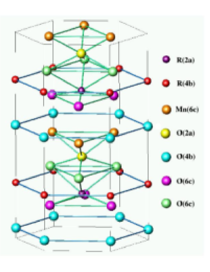
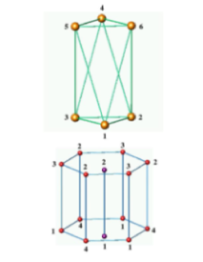
Figure 1: a) Atomic positions in a single hexagonal primitive cell of RMnO₃. b) Numbered Mn ions at the (6c) positions (top) and rare earth ions at the (4b) and (2a) positions (bottom).

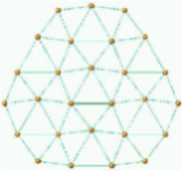
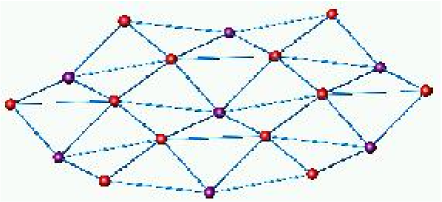
Figure 2: Triangular lattices formed by a) Mn ions (viewed parallel to the $c$-axis) and b) rare earth ions (viewed at an angle with respect to the $c$-axis).

The point group C_6v has four one-dimensional irreducible representations (IR’s), A₁, A₂, B₁ and B₂, and two two-dimensional IR’s E₁ and E₂. The same notation is used to label magnetic representations, where characters of ‘-1’ in the character table of C_6v indicate a combination of the point group element with time reversal [15]. For the 1D representations, the same names are given to the corresponding magnetic phases. In the presence of magnetic order parameters, the magnetic space groups are P6₃cm (A₁), P6₃c̱m̱ (A₂), P6̱₃cm̱ (B₁), and P6̱₃c̱m (B₂).

The spin configurations of rare-earth and Mn ions may be classified according to the magnetic representations by which they transform. All configurations which transform according to 1D representations are listed in Table 1, where the spin subscripts refer to the atom numbers shown in Figure 1b). The remaining degrees of freedom are accommodated by the 2D representations of C_6v; but so far, there is no evidence that phases corresponding to 2D OP’s appear in the phase diagram, so the 2D spin configurations are not included here.

R (2a)	A${}_{2}\;\;$	$S_{1z}+S_{2z}$
	B1	$S_{1z}-S_{2z}$
R (4b)	A1	$S_{1z}+S_{2z}-S_{3z}-S_{4z}$
	A2	$S_{1z}+S_{2z}+S_{3z}+S_{4z}$
	B1	$S_{1z}-S_{2z}-S_{3z}+S_{4z}$
	B2	$S_{1z}-S_{2z}+S_{3z}-S_{4z}$
Mn (6c)	A1	$-(S_{1x}-S_{4x})+\frac{1}{2}(S_{2x}+S_{3x}-S_{5x}-S_{6x})$
		$+\frac{\sqrt{3}}{2}(-S_{2y}+S_{3y}+S_{5y}-S_{6y})$
	A2	$-(S_{1y}-S_{4y})+\frac{\sqrt{3}}{2}(S_{2x}-S_{3x}-S_{5x}+S_{6x})$
		$+\frac{1}{2}(S_{2y}+S_{3y}-S_{5y}-S_{6y})$
	B1	$-(S_{1y}+S_{4y})+\frac{\sqrt{3}}{2}(S_{2x}-S_{3x}+S_{5x}-S_{6x})$
		$+\frac{1}{2}(S_{2y}+S_{3y}+S_{5y}+S_{6y})$
	B2	$-(S_{1x}+S_{4x})+\frac{1}{2}(S_{2x}+S_{3x}+S_{5x}+S_{6x})$
		$+\frac{\sqrt{3}}{2}(-S_{2y}+S_{3y}-S_{5y}+S_{6y})$
	A2	$S_{1z}+S_{2z}+S_{3z}+S_{4z}+S_{5z}+S_{6z}$
	B1	$S_{1z}+S_{2z}+S_{3z}-S_{4z}-S_{5z}-S_{6z}$

Table 1: 1D spin configurations classified by irreducible representation. The rare earth spin configurations are shown in Figure 4 and the first four Mn (6c) configurations are shown in Figure 3.

We now discuss general features of the H-T phase diagrams of RMnO₃ by considering the relative strength of the nearest-neighbour antiferromagnetic interaction for each spin configuration in Table 1. The antiferromagnetic interaction is defined as

$$I=\frac{1}{2}J\sum_{<ij>}\hat{S}_{i}\cdot\hat{S}_{j}$$ (1)

where the sum is over nearest neighbours and $\hat{S}_{i}$ is a spin operator. The parameter $J$ depends on the distance between nearest neighbours.

The first four configurations for Mn ions listed in Table 1 and illustrated in Figure 3, confine the spins to the hexagonal plane. The $B_{2}$ phase that appears below $T_{c}$, the $A_{2}$ phase found in magnetic fields, and the $B_{1}$ phase found at lower temperature in HoMnO₃ are due to these configurations. In order to compare the AF interaction strengths for the different configurations, first, sets of nearest neighbours should be separated into three cases, according to symmetry. The first case is the set of co-planar nearest neighbours ($\{1,2,3\}$ and $\{4,5,6\}$, numbered as in Figure 1b)). In this case, the AF interaction is the same for all four configurations, $I=-Js^{2}$. The second and third cases involve non-coplanar pairs. The second case pairs ions on opposite sides of the hexagonal primitive cell ($\{1,4\}$, $\{2,5\}$, $\{3,6\}$) and the third case is the remaining pairs. The second case favours $A_{1}$ and $A_{2}$ equally, while the third case favours $B_{1}$ and $B_{2}$ equally, with $I=\pm Js^{2}$ in both cases. The distance between partners in each pair for the second and third cases is exactly the same if the Mn position parameter $x$ is exactly $1/3$. Deviations away from $x=1/3$ will favour either the $A$ phases or the $B$ phases. However, the observed behaviour is the opposite of what could be expected. At higher temperatures (75 K) $x=0.338(1)$ [4], which brings the second case pairs closer together and favours the $A$ phases, but the $B_{2}$ phase is observed. At the lowest temperature (1.5 K) $x=0.330(1)$ the $B$ phases are favoured but the $A_{1}$ phase is observed. The subtle competition between all four phases which results in the dominance of the $B_{2}$ phase at high temperatures is most likely to be resolved by the inclusion of other interactions, such as next-nearest-neighbour, or interactions with the rare-earth ions.

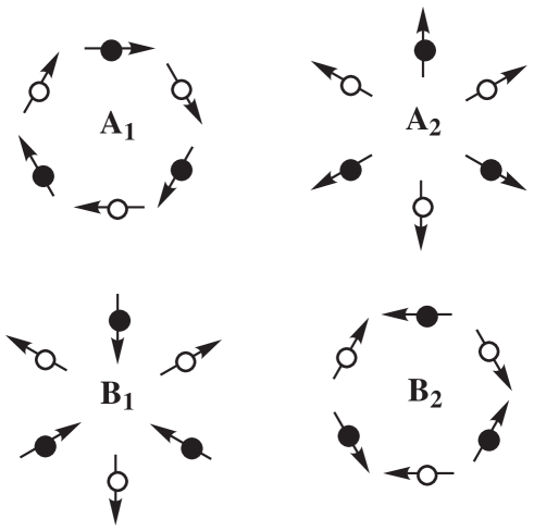
Figure 3: Manganese spin configurations in the hexagonal plane. These correspond to the first four (6c) configurations listed in Table 1 (after [1]).

In HoMnO₃, additional phases $B_{1}$ followed by $A_{1}$ appear as the temperature is further lowered. The $B_{1}$ phase is associated both with in-plane Mn moments and Ho ordering along the $c$-axis. The (2a) and (4b) holmium ions are almost co-planar. The $B_{1}$ phase is AF along the $c$-axis for (2a) and (4b) ions, but inside the hexagonal plane, the (4b) ions are aligned ferromagnetically with each other, and antiferromagnetically with the (2a) ions. This is shown in Figure 4b).

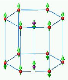
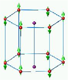
Figure 4: Rare earth spin configurations for a) $A_{1}$, b) $B_{1}$ and c) $B_{2}$ configurations for (2a) and (4b) positions listed in Table 1.

At the lowest temperatures, the $A_{1}$ configuration emerges, which has AF ordering of the (4b) spins in in the planes and along the $c$-axis, as shown in Figure 4a). Then, there can be no AF arrangement with respect to the (2a) positions (because there is no $A_{1}$ configuration for them). The phase transition from $B_{1}$ to $A_{1}$ is first-order, as is the case between all transitions involving different order parameters, therefore hysteresis is anticipated, both on phenomenological grounds, and also because of the persistence of the $B_{1}$ configuration on the (2a) positions.

The total in-plane AF interaction energy for all Ho ions is approximately the same for all three configurations shown in Figure 4. In all cases $I=-2Js^{2}$, but $J$ differs according to the distance between ions. If the (2a) and (4b) position parameters $z$ are equal then the three phases are degenerate, otherwise $A_{1}$ and $B_{2}$ have lower energy. The co-linear AF interactions favour the $B_{1}$ configuration, with $I=-3Js^{2}$ (versus $I=-2Js^{2}$ for $A_{1}$ and $I=2Js^{2}$ for $B_{2}$).

The $A_{2}$ phase will always dominate at high enough magnetic fields, since it transforms in the same way as the applied field, and couples linearly in the phenomenological sense. Microscopically, Zeeman coupling to Mn or Ho spins induces ferromagnetic order associated with the $A_{2}$ phase.

3 Landau Model and Phase Diagram

The order parameters of the phases A₁, A₂, B₁ and B₂ are denoted by $\eta_{1}$, $\eta_{2}$, $\eta_{3}$ and $\eta_{4}$, respectively. The minimal Landau model which describes the A₂ and B₂ phases, observed in all RMnO₃, is

$$F=\alpha_{2}\eta_{2}^{2}+\beta_{2}\eta_{2}^{4}+\alpha_{4}\eta_{4}^{2}+\beta_{4}\eta_{4}^{4}+\gamma_{24}\eta_{2}^{2}\eta_{4}^{2}-H_{z}(\rho_{1}\eta_{2}+\rho_{2}\eta_{2}^{3}+\rho_{3}\eta_{2}\eta_{4}^{2})$$ (2)

where where $\alpha_{i}$, $\beta_{i}$ and $\gamma_{ij}$ and $\rho_{i}$ are phenomenological coupling constants and $H_{z}$ is the magnetic field parallel to the $c$-axis. The coefficients $\alpha_{i}$ are temperature dependent, $\alpha_{i}=a_{i}(T-T_{i})$, where $T_{i}$ is the temperature limit of stability for each phase (which for convenience, we call the “transition temperature”), and $\beta_{i}>0$ is required for stability. $\alpha_{4}$ changes sign at $T_{N}\approx 100$K in all RMnO₃.

In zero applied field, the model allows for four different phases: $(0,0)$ (the parent phase), which may be connected to either $(\eta_{2},0)$ (A₂-phase), $(0,\eta_{4})$ (B₂-phase) or $(\eta_{2},\eta_{4})$ (mixed phase) by second order phase transitions. These are found by solving the set of coupled equations $\partial F/\partial\eta_{i}=0$, subject to the minimisation conditions $(\partial^{2}F/\partial\eta_{2}^{2})>0$ and $(\partial^{2}F/\partial\eta_{2}^{2})(\partial^{2}F/\partial\eta_{4}^{2})-(\partial^{2}F/\partial\eta_{2}\partial\eta_{4})^{2}>0$. The model also allows for the coexistence of two or more different phases by hysteresis.

The mixed phase $(\eta_{2},\eta_{4})$ can be a minimum of $F$ only when $4\beta_{2}\beta_{4}>\gamma_{24}^{2}$. Its existence is not the result of hysteresis. Anomalies in the $c$-axis magnetisation at the B₂ phase boundary [5] are evidence that $B_{2}$ and $A_{2}$ are coupled (i.e. $\gamma_{24}\neq 0$). In general, $\eta_{2}$ grows linearly with applied field but it may still be subject to a transition in the sense that a change in sign of $\alpha_{2}$ will increase the number of minima of the Landau functional.

Additional order parameters $\eta_{1}$ and $\eta_{3}$ are required to describe the additional phases observed in HoMnO₃. Additional terms in the free energy include those obtained by replacing in (2) $\eta_{4}^{2}$ by $\eta_{1}^{2}$ and $\eta_{3}^{2}$, as well as terms of the form $\eta_{1}\eta_{2}\eta_{3}\eta_{4}$ and $H_{z}\eta_{1}\eta_{3}\eta_{4}$.

The Landau model describing A₁, A₂, B₁ and B₂ phases is

$$F(\eta_{1},\eta_{2},\eta_{3},\eta_{4}) = F(\eta_{2},\eta_{4})+\alpha_{1}\eta_{1}^{2}+\beta_{1}\eta_{1}^{4}+\alpha_{3}\eta_{3}^{2}+\beta_{3}\eta_{3}^{4}+\gamma_{12}\eta_{1}^{2}\eta_{2}^{2}$$ (3)

$$+\gamma_{13}\eta_{1}^{2}\eta_{3}^{2}+\gamma_{14}\eta_{1}^{2}\eta_{4}^{2}+\gamma_{23}\eta_{2}^{2}\eta_{3}^{2}+\gamma_{34}\eta_{3}^{2}\eta_{4}^{2}+\gamma\eta_{1}\eta_{2}\eta_{3}\eta_{4}$$

$$-H_{z}(\rho_{4}\eta_{2}\eta_{3}^{2}+\rho_{5}\eta_{2}\eta_{1}^{2}+\rho_{6}\eta_{1}\eta_{3}\eta_{4})$$

This model may be solved exactly in zero applied field, and it is found that the allowed phases are $(0,0,0,0)$ (the parent phase), $(\eta_{1},0,0,0)$ etc. (A_i or B_i) and $(\eta_{1},\eta_{2},0,0)$ etc. (mixed phases involving two order parameters). In addition, two or more phases may co-exist due to hysteresis.

The models (2) and (3) were analysed by varying the temperature and field and searching for the minima of $F$ numerically. Typically, several minima were present, the deepest corresponding to the true ground state and the rest to metastable states observed as hysteresis. Each set of parameters $\alpha$, $\beta$, $\gamma$ and $\rho$ yields a different phase diagram; these parameters were varied to find the best match to phase diagrams obtained in experiments [1, 5, 12, 16].

Figure 5 shows numerical simulations of the phase diagrams for RMnO₃, modeled by (2). In all four diagrams, the onset of the $B_{2}$ phase for $H=0$ is determined by setting $T_{4}=80$ K. Below this temperature two minima corresponding to non-zero $\eta_{4}$ occur in (2). The $A_{2}$ phase, which dominates the right side (high field region) of all diagrams, corresponds to a Landau functional which has only one minimum that is shifted away from $\eta_{2}=0$ because of the term $H_{z}\eta_{2}$. Thus the free energy resembles the parent phase but the symmetry is $A_{2}$. In Figures 5b), c) and d) hysteresis occurs, indicated by lighter coloured areas near the black phase boundary line. Here the free energy has three minima, one corresponding to the field-shifted parent phase, and two to the $B_{2}$ phase. In Figures 5a), b) and d) we have $\gamma_{24}^{2}<4\beta_{2}\beta_{4}$, so a pair of minima for $\eta_{2}\neq 0$ never occurs. However, in Figure 5c), $\gamma_{24}^{2}>4\beta_{2}\beta_{4}$, so two shallow minima for $\eta_{2}$ co-exist with two for $\eta_{4}$ in the bottom left corner of the phase diagram. Figure 5b) shows the correct arrangement of phases on the phase diagram compared to experiments, but fails to simulate correctly the curvature of the phase boundary. Fig ure 5d), which includes the non-linear (in OP) field-dependent terms in (2), is a significant improvement.

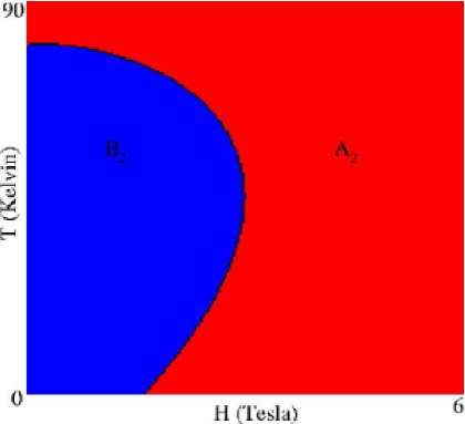
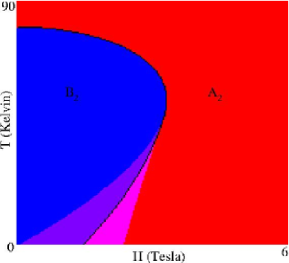
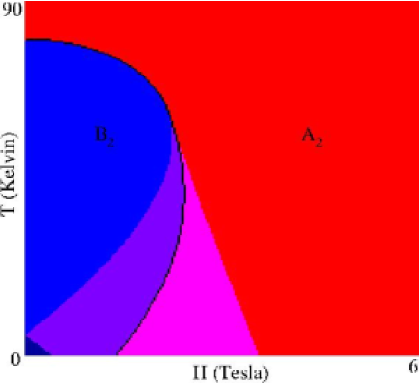
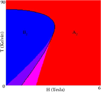
Figure 5: Numerical simulations of the phase diagram of RMnO₃. The black line is the boundary between the $A_{2}$ and $B_{2}$ phases. Hysteresis occurs in the lighter-coloured regions. In all four diagrams $T_{4}=80$ K, $T_{2}=10$ K, $\beta_{2}=10$, $\beta_{4}=100$ and $\rho_{1}=12$, while $\gamma_{24}=60$, 150, 300 and 150 in (a), (b), (c) and (d) respectively. The parameters $a_{i}$ ($\alpha_{i}=a_{i}(T-T_{i})$) were scaled to unity. Nonlinear field-dependent coefficients $\rho_{2}=\rho_{3}=5$ are introduced in diagram (d).

Figure 6 shows numerical simulations of the phase diagram of HoMnO₃, modeled by (3). The upper part of the diagrams, showing the $B_{2}$ and $A_{2}$ phases, is similar to RMnO₃, in that the $B_{2}$ phase appears below the transition temperature $T_{4}=75$ K, and the $A_{2}$ phase is induced by the magnetic field. Non-zero transition temperatures $T_{i}$ were assigned to all other phases ($T_{1}=52$ K, $T_{2}=39$ K, $T_{3}=62$ K) below which the phases are metastable and hysteresis occurs. True phase transitions occur below the transition temperatures, along the lines where the free energies, evaluated for different phases, are equal. Different shades within a single phase represent the presence of other, metastable phases. Figure 6a) bears a poor resemblance to experiments. Figure 6b), which includes non-linear field-dependent terms, is significantly better, but still fails to reproduce qualitatively all of the phase boundary around the $B_{1}$ phase as seen in experiments.

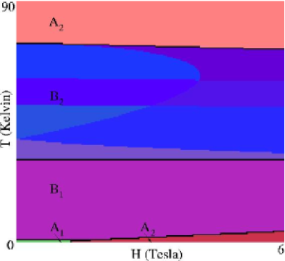
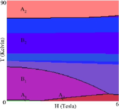
Figure 6: Numerical simulations of the phase diagram of HoMnO₃. Black lines separate the phases, while different shades within a phase represent the presence of other meta-stable states. In both diagrams $\beta_{1}=0.14$, $\beta_{2}=0.08$, $\beta_{3}=0.2$, $\beta_{4}=0.4$, while $\gamma_{12}=1$, $\gamma_{13}=1$, $\gamma_{14}=1$, $\gamma_{23}=6$, $\gamma_{24}=2.9$, $\gamma_{34}=10$, $\rho_{1}=1$ in (a) and $\gamma_{12}=90$, $\gamma_{13}=\gamma_{14}=\gamma_{23}=\gamma_{24}=\gamma_{34}=100$, $\rho_{1}=4$ in (b). Diagram (b) also includes non-linear field-dependent terms $\rho_{2}=1$, $\rho_{3}=2$, $\rho_{4}=0.05$.

4 Discussion

In Section 2 we argued that even in the absence of true geometrical frustration, there is not enough information to predict the magnetic ground state without detailed knowledge of the AF interaction strength $J$. In Landau theory, the microscopic model (1) is replaced by a phenomenological one (2,3), and the parameter $J$ is incorporated into the temperature-dependent $\alpha_{i}$. Landau theory includes all interactions allowed by symmetry, and as such is more general than the AF interaction, which is isotropic. However, the proliferation of phenomenological constants also inhibits the predictive powers of the Landau model. Nevertheless, Landau modeling is useful because it can reveal the minimal elements in a theory that are needed to describe the phase diagrams of RMnO₃. In our analysis, we found that a model based on the usual second and fourth order terms, and a linear coupling of the order parameter to the magnetic field, does not describe well the observed phase diagrams, especially the curvature of the phase boundaries. The inclusion of non-linear (in OP) field-dependent terms is a significant improvement.

The magneto-electric effect is observed in the region between the $B_{1}$ and $B_{2}$ phases. Linear coupling of the magnetic and electric fields of the form $\alpha_{ij}E_{i}B_{j}$ can only occur when both inversion and time reversal symmetry are absent - these are necessary but not sufficient conditions. A mixture of $B_{1}$ and $B_{2}$ order parameters (due to hysteresis) does not lower the symmetry enough for magneto-electric coupling. However, domain walls, which connect different domains of the same phase, have been implicated in the observation of the magneto-electric effect [6]. Thus OP gradient terms, which couple to the magnetic field, may significantly alter the free energy landscape, and could possibly replace the non-linear field-dependent terms which we introduced.

In conclusion, we have studied phase diagrams for RMnO₃, using group theory and Landau theory, by including up to fourth order phenomenological couplings between order parameters and non-linear coupling to an applied magnetic field. Antiferromagnetic competition between magnetic phases, due to a near perfect triangular lattice structure, gives rise to a complex phase diagram. Our simulations reproduce the main features seen in experimental results, including the general arrangement of phases on the diagram, hysteresis effects and the curvature of phase boundaries.

References

- [1] M. Fiebig and Th. Lottermoser, J. Appl. Phys. 93, 8194 (2003).
- [2] D. Fröhlich, St. Leute, V. V. Pavlov, R. V. Pisarev and K. Kohn, J. Appl. Phys. 85, 4762 (1999).
- [3] M. Fiebig, D. Fröhlich, K. Kohn, Th. Lottermoser, V. V. Pavlov and R. V. Pisarev, Phys. Rev. Lett. 84, 5620 (2000).
- [4] Th. Lonkai, D. Hohlwein, J. Ihringer and W. Prandl, Appl. Phys. A 74, S843 (2002).
- [5] B. Lorenz, F. Yen, M. M. Gospodinov and C. W. Chu, Phys. Rev. B 71, 014438 (2005).
- [6] Th. Lottermoser and M. Fiebig, Phys. Rev. B 70, 220407 (2004).
- [7] M. Fiebig, J. Phys. Appl. Phys: D 38, R123 (2005).
- [8] C. dela Cruz, F. Yen, B. Lorenz, Y. Q. Wang, Y. Y. Sun, M. M. Gospodinov and C. W. Chu, Phys. Rev. B 71, 060407 (2005).
- [9] M. Fiebig, C. Degenhardt and R. V. Pisarev, J. Appl. Phys. 91, 8867 (2002).
- [10] B. Lorenz, A. P. Litvinchuk, M. M. Gospodinov and C. W. Chu, Phys. Rev. Lett. 92, 87204 (2004).
- [11] T. Lottermoser, T. Lonkai, U. Amann, D. Hohwein, J. Ihringer and M. Fiebig, Nature 430, 541 (2004).
- [12] O. P. Vajik, M. Kenzelmann, J. W. Lynn, S. B. Kim and S. W. Cheong, Phys. Rev. Lett. 94, 087601 (2005).
- [13] A preliminary version of this work appeared in S. H. Curnoe and I. Munawar, Proceedings of SCES ’05, Physica B 378-380, 554 (2006).
- [14] H. L. Yakel, W. C. Koehler, E. F. Bertaut and E. F. Forrat, Acta Crystallogr. 16, 957 (1963).
- [15] We use the notation found in M. Tinkham, Group Theory and Quantum Mechanics (McGraw-Hill, 1964) and International Tables for Crystallography (Kluwer, 2002).
- [16] F. Yen et al. Phys. Rev. B 71, 180407 (2005).