A novel choice of the graphene unit vectors,
useful in zone-folding computations

Abstract

The dispersion relations of carbon nanotubes are often obtained cross-sectioning those of graphene (zone-folding technique) in a rectangular region of the reciprocal space, where it is easier to fold the resulting relations into the nanotube Brillouin zone. We propose a particular choice of the unit vectors for the graphene lattice, which consists of the symmetry vector and the translational vector of the considered carbon nanotube. Due to the properties of the corresponding unit vectors in the reciprocal space, this choice is particularly useful for understanding the relationship between the rectangular region where the folding procedure is most easily applied and the overall graphene reciprocal space. Such a choice allows one to find, from any graphene wave vector, the equivalent one inside the rectangular region in a computationally inexpensive way. As an example, we show how the use of these unit vectors makes it easy to limit the computation to the bands nearest to the energy maxima and minima when determining the nanotube dispersion relations from those of graphene with the zone-folding technique.

I Introduction

Carbon nanotubes are cylindrical structures with diameters that are usually in the few nanometer range and lengths up to tens of microns. Due to their high mechanical strength and thermal conductivity and to their unusual electronic properties, carbon nanotubes constitute a very promising material for many applications meyyappan ; ajayan , such as active devices, intra-chip interconnections, field emitters, antennas, sensors, scanning probes, reinforcement for composite materials, energy and hydrogen storage. In particular, from the electronic point of view, they can behave as metallic or semiconducting materials, depending on their geometrical properties hamada ; mintmire ; saito1 ; saito .
A single-wall carbon nanotube can be described as a graphene sheet rolled, along one of its lattice vectors (the so-called chiral vector), into a cylindrical shape. As a consequence of the closure boundary condition along the chiral vector, only a subset of graphene wave vectors, located on parallel lines, are allowed. Therefore the dispersion relations of carbon nanotubes are often found cross-sectioning those of graphene along such lines (zone-folding technique) saito ; reichbook . The cross-sections are usually taken in a particular rectangular region of the graphene reciprocal space (which can be seen as a primitive unit cell of the graphene reciprocal lattice).
Here we introduce an unusual choice of the unit vectors in the graphene direct and reciprocal space, which, as a result of a direct geometrical relation with such a rectangle, makes it clearer how the overall reciprocal space can be obtained by replicating the rectangle.
This allows a more complete understanding of the results of the zone-folding method, explaining, for example, how the periodicity of the nanotube energy bands arises from the computational procedure.
We also show how such unit vectors make it easy to find, from any point of interest of the graphene reciprocal space, the equivalent wave vector located inside the above-mentioned rectangular region. At the end of the present communication, we apply this procedure to the graphene degeneration points, in order to compute just the nanotube bands nearest to the energy maxima and minima.
In Figs. 1 and 2 we show the graphene lattice in the direct and reciprocal space, respectively, and the $(\hat{x},\hat{y})$ reference frame that we have used in the following. The graphene lattice structure in the real space can be seen as the replication of the graphene rhomboidal unit cell shown in Fig. 1 (containing two inequivalent carbon atoms $A$ and $B$) through linear combinations with integer coefficients of the lattice unit vectors $\vec{a}_{1}=(\sqrt{3}a/2)\hat{x}+(a/2)\hat{y}$ and $\vec{a}_{2}=(\sqrt{3}a/2)\hat{x}-(a/2)\hat{y}$. Correspondingly, the unit vectors of the graphene reciprocal lattice are $\vec{b}_{1}=(2\pi/(\sqrt{3}a))\hat{x}+(2\pi/a)\hat{y}$ and $\vec{b}_{2}=(2\pi/(\sqrt{3}a))\hat{x}-(2\pi/a)\hat{y}$, which are reported in Fig. 2, along with the graphene hexagonal Brillouin zone.
An $(n,m)$ carbon nanotube is obtained rolling up a graphene sheet along its chiral vector $\vec{C}_{h}=n\vec{a}_{1}+m\vec{a}_{2}$; the circumference of the nanotube is consequently equal to the length of this vector: $L=|\vec{C}_{h}|=a\sqrt{n^{2}+m^{2}+nm}$.
If we define $d_{R}$ as the greatest common divisor of $2m+n$ and $2n+m$, we have that the lattice unit vector of the nanotube (which represents a 1D lattice) is the so-called translational vector $\vec{T}=t_{1}\vec{a}_{1}+t_{2}\vec{a}_{2}$ of the unrolled graphene sheet, parallel to the nanotube axis and orthogonal to $\vec{C}_{h}$, where $t_{1}$ and $t_{2}$ are relatively prime integer numbers given by $t_{1}=(2m+n)/d_{R}$ and $t_{2}=-(2n+m)/d_{R}$. Therefore, the rectangle having as edges the chiral vector $\vec{C}_{h}$ and the translational vector $\vec{T}$ represents the unit cell of the nanotube, which repeats identically along the nanotube axis with a lattice unit vector $\vec{T}$, the length of which is equal to $T=|\vec{T}|=\sqrt{3}L/d_{R}$. The number of graphene unit cells inside the nanotube unit cell is equal to $N=2L^{2}/(a^{2}d_{R})$.
The coordinates of all the $N$ points identifying the graphene unit cells inside the rectangular region representing the nanotube unit cell in the unrolled graphene sheet are defined (apart from translations by an integer number of $\vec{C}_{h}$ and $\vec{T}$ vectors) by integer multiples of the so-called symmetry vector $\vec{R}=p\vec{a}_{1}+q\vec{a}_{2}$, where $p$ and $q$ are two relatively prime integer numbers, univocally determined by the two relations: $t_{1}q-t_{2}p=1$ and $0<M\leq N$ (where we define the quantity $M=mp-nq$). In particular, we have that $N\vec{R}=\vec{C}_{h}+M\vec{T}$ saito .
In Fig. 1 we show all of these vectors in the direct space for the nanotube $(10,0)$ (for which $\vec{C}_{h}=10\vec{a}_{1}$, $L=10a$, $d_{R}=10$, $\vec{T}=\vec{a}_{1}-2\vec{a}_{2}$, $T=\sqrt{3}a$, $N=20$, $\vec{R}=\vec{a}_{1}-\vec{a}_{2}$ and $M=10$).

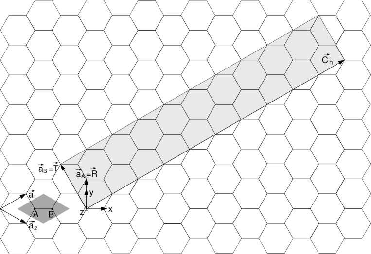
Figure 1: The described quantities in the direct space for a $(10,0)$ nanotube. The heavy-shaded rhombus is the graphene unit cell, while the light-shaded rectangle represents (once the graphene sheet has been rolled up) the nanotube unit cell.

Since in the direct space the nanotube is a one-dimensional lattice with a unit vector $\vec{T}$ and with a $T$ wide unit cell along the nanotube axis, in the reciprocal space its unit vector is equal to $\vec{K}_{2}=(2\pi/T)\hat{T}=(m\vec{b}_{1}-n\vec{b}_{2})/N$ and its Brillouin zone is represented by the values of the wave vector $k$ (along the nanotube axis) which satisfy the inequality $-\pi/T<k\leq\pi/T$.
Many physical properties of the nanotubes, such as the energy dispersion relations, can be found from the corresponding quantities of graphene using the zone-folding technique saito ; reichbook . Indeed, as a consequence of the closure of the graphene sheet to form the carbon nanotube, we have to enforce that the graphene electron wave function $e^{i\vec{k}\cdot\vec{r}}u(\vec{k})$ (where $u(\vec{k})$ is a Bloch lattice function) has identical values in any pair of points $\vec{r}$ and $\vec{r}+\vec{C}_{h}$. To satisfy the resulting relation $e^{i\vec{k}\cdot\vec{C}_{h}}=1$, the component along $\hat{C}_{h}$ of the wave vector has to be equal to an integer multiple of the vector $\vec{K}_{1}=(2\pi/L)\hat{C}_{h}=(-t_{2}\vec{b}_{1}+t_{1}\vec{b}_{2})/N$. If we cross-section the graphene dispersion relations in correspondence of the parallel lines (separated by a distance $|\vec{K}_{1}|=2\pi/L$) containing the allowed graphene wave vectors and we fold such sections into the nanotube Brillouin zone, we find the relations for the carbon nanotube. This procedure is applied to a region of the graphene reciprocal space containing all and only the inequivalent graphene wave vectors. In particular, the rectangle having as edges the vectors $N\vec{K}_{1}$ and $\vec{K}_{2}$ has these properties (as we have demonstrated in the Supplementary Information) and corresponds to the region that is usually implicitly chosen to apply the zone-folding method, because here, considering only the allowed graphene wave vectors, we obtain $N$ segments with a width equal to $2\pi/T$, that can be folded into the Brillouin zone of the nanotube by simply taking the component along $\hat{T}$ of each graphene wave vector (such a component becomes the nanotube wave vector).
In Fig. 2 we show the quantities in the reciprocal space for the nanotube $(10,0)$ (for which $\vec{K}_{1}=(2\pi/(10a))\hat{C}_{h}=(2\vec{b}_{1}+\vec{b}_{2})/20$ and $\vec{K}_{2}=(2\pi/(\sqrt{3}a))\hat{T}=-\vec{b}_{2}/2$).

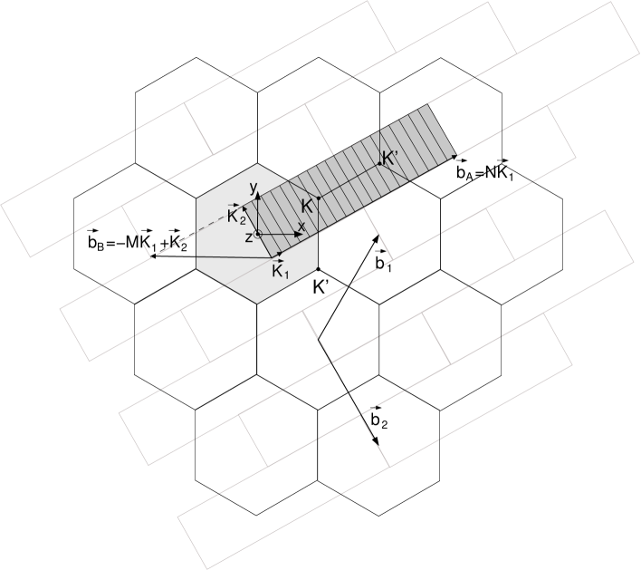
Figure 2: The described quantities in the reciprocal space for a $(10,0)$ nanotube. The light-shaded hexagon is the graphene Brillouin zone, while the heavy-shaded rectangle is the rectangular area specified by the vectors $N\vec{K}_{1}$ and $\vec{K}_{2}$.

We propose an alternative choice of the graphene unit vectors that allows to clarify the relation between the previously described rectangular region specified by the vectors $N\vec{K}_{1}$ and $\vec{K}_{2}$ and the overall graphene reciprocal space; in particular it makes it easy to find, for any given wave vector, the equivalent wave vector belonging to such a rectangular area. As we shall see, this can be very useful when we apply the zone-folding method cross-sectioning this rectangle.

II Alternative choice of the graphene unit vectors

Let us consider the graphene sheet forming, once rolled up, a carbon nanotube with chiral vector $\vec{C}_{h}$, translational vector $\vec{T}$ and symmetry vector $\vec{R}$. We propose, as an alternative choice of the graphene unit vectors in the direct space, exactly the pair of vectors $\vec{a}_{A}\equiv\vec{R}$ and $\vec{a}_{B}\equiv\vec{T}$:

$$\vec{a}_{A}\! = \!\vec{R}=p\vec{a}_{1}+q\vec{a}_{2}=\frac{a}{2}\sqrt{3}(p+q)\hat{x}+\frac{a}{2}(p-q)\hat{y}$$ (1)

$$\vec{a}_{B}\! = \!\vec{T}=t_{1}\vec{a}_{1}+t_{2}\vec{a}_{2}=\frac{a}{2}\sqrt{3}(t_{1}+t_{2})\hat{x}+\frac{a}{2}(t_{1}-t_{2})\hat{y}\quad.$$ (2)

To verify that these two vectors can actually be used as graphene unit vectors in the direct space, we have to demonstrate that their linear combinations with integer coefficients yield all and only the lattice vectors of such a space, i.e. the vectors that are also linear combinations with integer coefficients of $\vec{a}_{1}$ and $\vec{a}_{2}$.
Since both $\vec{R}$ and $\vec{T}$ are linear combinations with integer coefficients of $\vec{a}_{1}$ and $\vec{a}_{2}$, every linear combination with integer coefficients of $\vec{R}$ and $\vec{T}$ is also a linear combination with integer coefficients of $\vec{a}_{1}$ and $\vec{a}_{2}$.
On the other hand, in order to demonstrate that every linear combination with integer coefficients of $\vec{a}_{1}$ and $\vec{a}_{2}$ is also a linear combination with integer coefficients of $\vec{R}$ and $\vec{T}$, it is useful to consider the linear system consisting of the two following known relations:

$$\left\{\begin{array}[]{l}p\vec{a}_{1}+q\vec{a}_{2}=\vec{R}\\ t_{1}\vec{a}_{1}+t_{2}\vec{a}_{2}=\vec{T}\\ \end{array}\right.\quad.$$ (3)

Solving for $\vec{a}_{1}$ and $\vec{a}_{2}$, we find that

$$\left\{\begin{array}[]{l}(-t_{2}p+qt_{1})\vec{a}_{1}=-t_{2}\vec{R}+q\vec{T}\\ (t_{1}q-pt_{2})\vec{a}_{2}=t_{1}\vec{R}-p\vec{T}\\ \end{array}\right.\quad\textrm{or equivalently}\quad\left\{\begin{array}[]{l}\vec{a}_{1}=-t_{2}\vec{R}+q\vec{T}\\ \vec{a}_{2}=t_{1}\vec{R}-p\vec{T}\\ \end{array}\right.$$ (4)

(recalling that $t_{1}q-t_{2}p=1$), which means that $\vec{a}_{1}$ and $\vec{a}_{2}$ are linear combinations with integer coefficients of $\vec{R}$ and $\vec{T}$. Consequently, also every linear combination with integer coefficients of $\vec{a}_{1}$ and $\vec{a}_{2}$ is a linear combination with integer coefficients of $\vec{R}$ and $\vec{T}$.
Using the coordinates of $\vec{R}$ and $\vec{T}$ in the $(\hat{x},\hat{y})$ reference frame of Fig. 1, and introducing a unit vector $\hat{z}$ that is orthogonal to the plane $\hat{x},\hat{y}$ of the graphene sheet and forms a right-hand reference frame $(\hat{x},\hat{y},\hat{z})$ with $\hat{x}$ and $\hat{y}$, we have that

$$\vec{T}\times\hat{z}\! = \!-\frac{a}{2}(t_{2}-t_{1})\hat{x}-\frac{a}{2}\sqrt{3}(t_{2}+t_{1})\hat{y}$$ (5)

$$\hat{z}\times\vec{R}\! = \!\frac{a}{2}(q-p)\hat{x}+\frac{a}{2}\sqrt{3}(q+p)\hat{y}$$ (6)

$$\vec{R}\cdot\left(\vec{T}\times\hat{z}\right)\! = \!\frac{a^{2}\sqrt{3}}{2}(t_{1}q-t_{2}p)=\frac{a^{2}\sqrt{3}}{2}\quad,$$ (7)

where we have used again the relation $t_{1}q-t_{2}p=1$. Therefore, the corresponding unit vectors of graphene in the reciprocal space are (using the well-known relations between the unit vectors in the direct and in the reciprocal space ashcroft ):

$$\vec{b}_{A}\! = \!2\pi\frac{\vec{a}_{B}\times\hat{z}}{\vec{a}_{A}\cdot(\vec{a}_{B}\times\hat{z})}=2\pi\frac{\vec{T}\times\hat{z}}{\vec{R}\cdot(\vec{T}\times\hat{z})}=-\frac{2\pi}{a\sqrt{3}}(t_{2}-t_{1})\hat{x}-\frac{2\pi}{a}(t_{2}+t_{1})\hat{y}=$$ (8)

$$= \!-t_{2}\left(\frac{2\pi}{\sqrt{3}a}\hat{x}+\frac{2\pi}{a}\hat{y}\right)+t_{1}\left(\frac{2\pi}{\sqrt{3}a}\hat{x}-\frac{2\pi}{a}\hat{y}\right)=-t_{2}\vec{b}_{1}+t_{1}\vec{b}_{2}=$$

$$= \!-t_{2}(n\vec{K}_{1}+t_{1}\vec{K}_{2})+t_{1}(m\vec{K}_{1}+t_{2}\vec{K}_{2})=(-t_{2}n+t_{1}m)\vec{K}_{1}=$$

$$= \!N\vec{K}_{1}=N\frac{2\pi}{L}\hat{C}_{h}$$

and

$$\vec{b}_{B}\! = \!2\pi\frac{\hat{z}\times\vec{a}_{A}}{\vec{a}_{A}\cdot(\vec{a}_{B}\times\hat{z})}=2\pi\frac{\hat{z}\times\vec{R}}{\vec{R}\cdot(\vec{T}\times\hat{z})}=\frac{2\pi}{a\sqrt{3}}(q-p)\hat{x}+\frac{2\pi}{a}(q+p)\hat{y}=$$ (9)

$$= \!q\left(\frac{2\pi}{\sqrt{3}a}\hat{x}+\frac{2\pi}{a}\hat{y}\right)-p\left(\frac{2\pi}{\sqrt{3}a}\hat{x}-\frac{2\pi}{a}\hat{y}\right)=q\vec{b}_{1}-p\vec{b}_{2}=$$

$$= \!q(n\vec{K}_{1}+t_{1}\vec{K}_{2})-p(m\vec{K}_{1}+t_{2}\vec{K}_{2})=(qn-pm)\vec{K}_{1}+(qt_{1}-pt_{2})\vec{K}_{2}=$$

$$= \!-M\vec{K}_{1}+\vec{K}_{2}=-M\frac{2\pi}{L}\hat{C}_{h}+\frac{2\pi}{T}\hat{T}\quad,$$

which are linear combinations with integer coefficients of the vectors $\vec{K}_{1}$ and $\vec{K}_{2}$ and have components along $\hat{C}_{h}$ and $\hat{T}$: $b_{A_{C}}=N(2\pi/L)$ ,  $b_{A_{T}}=0$ ,  $b_{B_{C}}=-M(2\pi/L)$ ,  $b_{B_{T}}=2\pi/T$ . To find the previous results we have used, besides the fact that $t_{1}q-t_{2}p=1$ and $M=mp-nq$, the relations: $-t_{2}n+t_{1}m=N$, $\vec{b}_{1}=n\vec{K}_{1}+t_{1}\vec{K}_{2}$ and $\vec{b}_{2}=m\vec{K}_{1}+t_{2}\vec{K}_{2}$.
Indeed, using the relations listed in the Introduction, we obtain that

$$mt_{1}-nt_{2}=m\frac{2m+n}{d_{R}}+n\frac{2n+m}{d_{R}}=\frac{2}{d_{R}}(m^{2}+nm+n^{2})=\frac{2}{d_{R}}\left(\frac{L}{a}\right)^{2}=N\quad.$$ (10)

The relations between the vectors $\vec{b}_{1}$ and $\vec{b}_{2}$ and the vectors $\vec{K}_{1}$ and $\vec{K}_{1}$ can instead be found starting from the identities:

$$\left\{\begin{array}[]{l}\displaystyle\vec{K}_{1}=\frac{1}{N}(-t_{2}\vec{b}_{1}+t_{1}\vec{b}_{2})\\ \\[-10.0pt] \displaystyle\vec{K}_{2}=\frac{1}{N}(m\vec{b}_{1}-n\vec{b}_{2})\\ \end{array}\right.$$ (11)

and solving for $\vec{b}_{1}$ and $\vec{b}_{2}$ this system of two equations. We find that

$$\left\{\begin{array}[]{l}(mt_{1}-nt_{2})\vec{b}_{1}=N(n\vec{K}_{1}+t_{1}\vec{K}_{2})\\ (mt_{1}-nt_{2})\vec{b}_{2}=N(m\vec{K}_{1}+t_{2}\vec{K}_{2})\\ \end{array}\right.$$ (12)

and thus (using the fact that $mt_{1}-nt_{2}=N$) that

$$\left\{\begin{array}[]{l}\displaystyle\vec{b}_{1}=n\vec{K}_{1}+t_{1}\vec{K}_{2}=n\frac{2\pi}{L}\hat{C}_{h}+t_{1}\frac{2\pi}{T}\hat{T}\\ \\[-10.0pt] \displaystyle\vec{b}_{2}=m\vec{K}_{1}+t_{2}\vec{K}_{2}=m\frac{2\pi}{L}\hat{C}_{h}+t_{2}\frac{2\pi}{T}\hat{T}\\ \end{array}\right.\quad.$$ (13)

From this result, it is also apparent that the components of $\vec{b}_{1}$ and $\vec{b}_{2}$ along $\hat{C}_{h}$ and $\hat{T}$ are: $b_{1_{C}}=n(2\pi/L)$ ,  $b_{1_{T}}=t_{1}(2\pi/T)$ ,  $b_{2_{C}}=m(2\pi/L)$ ,  $b_{2_{T}}=t_{2}(2\pi/T)$ .

III Applications

This choice of unit vectors helps us to understand the relation between the rectangular region having as edges the vectors $N\vec{K}_{1}$ and $\vec{K}_{2}$ and the overall graphene reciprocal space. Indeed, such a rectangular region contains all and only the inequivalent graphene wave vectors and can therefore be considered as a primitive unit cell of the graphene reciprocal lattice. In particular, considering as unit vectors of the graphene reciprocal space $\vec{b}_{A}$ and $\vec{b}_{B}$ (which have a clear geometrical relation with the considered region), we have that the overall reciprocal space can be spanned translating the rectangular region by vectors that are linear combinations, with integer coefficients, of $\vec{b}_{A}$ (which is exactly equal to $N\vec{K}_{1}$, the base of the rectangle) and $\vec{b}_{B}$ (which has a component along $\hat{T}$ equal to $|\vec{K}_{2}|$, the height of the rectangle, and a component along $\hat{C}_{h}$ equal to $-M|\vec{K}_{1}|$, i.e. an integer number of times the distance $|\vec{K}_{1}|$ between the segments along which we take the $N$ cross-sections inside the rectangle in the zone-folding method). Therefore, the overall graphene reciprocal space is spanned by rows (parallel to $\hat{C}_{h}$) of equivalent rectangles, with each row shifted along $\hat{C}_{h}$ by $-M\vec{K}_{1}$ with respect to the adjacent one (as we show in gray in Fig. 2 for the particular case of a (10,0) nanotube, where $M=10$, $N=20$ and therefore $N=2M$).
This clarifies the result obtained by cross-sectioning the graphene dispersion relations along the $N$ parallel lines (separated by a distance $|\vec{K}_{1}|$) to which the $N$ parallel segments used in the zone-folding method belong. Since the parallel rows of rectangles spanning the graphene reciprocal space have a nonzero relative shift along $\hat{C}_{h}$ (and therefore the generic graphene wave vectors $\vec{k}$ and $\vec{k}+\vec{K}_{2}$ are not equivalent), the relation obtained from each single cross-section in general is not periodic with period equal to $|\vec{K}_{2}|$ (the width of the nanotube Brillouin zone). Nevertheless, since the relative shift along $\hat{C}_{h}$ between rows of rectangles is an integer multiple of the distance $|\vec{K}_{1}|$ between the $N$ parallel lines, we find, starting from a wave vector $\vec{k}$ on one of the $N$ lines and moving by $|\vec{K}_{2}|$ along $\hat{T}$ and by a proper multiple of $|\vec{K}_{1}|$ along $\vec{C}_{h}$, a wave vector equivalent to $\vec{k}$ on another of the $N$ lines of allowed wave vectors. Therefore the overall set of relations, obtained drawing all the $N$ cross-sections on the same one-dimensional domain, is indeed periodic with period $|\vec{K}_{2}|$. This is in agreement with the fact that the resulting relations are the nanotube dispersion relations, that have to be periodic with a period equal to the width of the nanotube Brillouin zone.
The proposed alternative choice of graphene unit vectors is particularly useful for the determination, for any given wave vector, of the equivalent wave vector within the previously discussed rectangular region of the graphene reciprocal space.
Indeed, given a graphene wave vector $\vec{k}$, if we use $\vec{b}_{A}$ and $\vec{b}_{B}$ as unit vectors in the reciprocal space, all the wave vectors equivalent to $\vec{k}$ can be written as $\vec{k}^{eq}=\vec{k}+\alpha\vec{b}_{A}+\beta\vec{b}_{B}$, with $\alpha$ and $\beta$ integer numbers. Thus the corresponding components $k^{eq}_{C}$ and $k^{eq}_{T}$ along $\hat{C}_{h}$ and $\hat{T}$, respectively, are:

$$\left\{\begin{array}[]{l}\displaystyle k^{eq}_{C}=k_{C}+\alpha b_{A_{C}}+\beta b_{B_{C}}=k_{C}+\alpha N\frac{2\pi}{L}-\beta M\frac{2\pi}{L}\\ \\[-10.0pt] \displaystyle k^{eq}_{T}=k_{T}+\alpha b_{A_{T}}+\beta b_{B_{T}}=k_{T}+\beta\frac{2\pi}{T}\end{array}\right.\quad.$$ (14)

Since we want to find the particular $\vec{k}^{eq}$ belonging to the rectangular region, such components have to satisfy the following relations:

$$\left\{\begin{array}[]{l}\displaystyle 0\leq k^{eq}_{C}<N\frac{2\pi}{L}\\ \\[-10.0pt] \displaystyle-\frac{\pi}{T}<k^{eq}_{T}\leq\frac{\pi}{T}\end{array}\right.\quad\textrm{or equivalently}\quad\left\{\begin{array}[]{l}\displaystyle 0\leq k^{eq}_{C}<N\frac{2\pi}{L}\\ \\[-10.0pt] \displaystyle 0<k^{eq}_{T}+\frac{\pi}{T}\leq\frac{2\pi}{T}\end{array}\right.\quad.$$ (15)

Substituting the expressions of $k^{eq}_{C}$ and $k^{eq}_{T}$ into these inequalities, we find:

$$\left\{\begin{array}[]{l}\displaystyle 0\leq\left(k_{C}-\beta M\frac{2\pi}{L}\right)+\alpha N\frac{2\pi}{L}<N\frac{2\pi}{L}\\ \\[-10.0pt] \displaystyle 0<\left(k_{T}+\frac{\pi}{T}\right)+\beta\frac{2\pi}{T}\leq\frac{2\pi}{T}\end{array}\right.$$ (16)

and thus

$$\left\{\begin{array}[]{l}\displaystyle-\alpha\left(N\frac{2\pi}{L}\right)\leq k_{C}-\beta M\frac{2\pi}{L}<(-\alpha+1)\left(N\frac{2\pi}{L}\right)\\ \\[-10.0pt] \displaystyle-\beta\left(\frac{2\pi}{T}\right)<k_{T}+\frac{\pi}{T}\leq(-\beta+1)\left(\frac{2\pi}{T}\right)\end{array}\right.$$ (17)

or equivalently

$$\left\{\begin{array}[]{l}\displaystyle-\alpha\leq\frac{k_{C}-\beta M(2\pi/L)}{N(2\pi/L)}<-\alpha+1\\ \\[-10.0pt] \displaystyle-\beta<\frac{k_{T}+(\pi/T)}{2\pi/T}\leq-\beta+1\end{array}\right.\quad.$$ (18)

The values of $\alpha$ and $\beta$, and consequently the vector $\vec{k}^{eq}$, can be easily found using the fact that the second inequality contains only $\beta$. Indeed, from the second inequality we find that (using the ceiling and floor functions):

$$\beta=\left\{\begin{array}[]{ll}\displaystyle-\left\lceil\,\frac{k_{T}+(\pi/T)}{2\pi/T}\,\right\rceil+1&\textrm{if \ $\displaystyle k_{T}+\frac{\pi}{T}\geq 0$ }\\ \\[-10.0pt] \displaystyle\left\lfloor\frac{|k_{T}+(\pi/T)|}{2\pi/T}\right\rfloor+1&\textrm{if \ $\displaystyle k_{T}+\frac{\pi}{T}<0$ }\end{array}\right.\quad.$$ (19)

Once the value of $\beta$ is found, the quantity $k_{C}-\beta M(2\pi/L)$ in the first inequality is known and thus from first inequality we obtain that:

$$\alpha=\left\{\begin{array}[]{ll}\displaystyle-\left\lfloor\frac{k_{C}-\beta M(2\pi/L)}{N(2\pi/L)}\right\rfloor&\textrm{if \ $\displaystyle k_{C}-\beta M\frac{2\pi}{L}\geq 0$ }\\ \\[-10.0pt] \displaystyle\left\lceil\,\frac{|k_{C}-\beta M(2\pi/L)|}{N(2\pi/L)}\,\right\rceil&\textrm{if \ $\displaystyle k_{C}-\beta M\frac{2\pi}{L}<0$ }\end{array}\right.\quad.$$ (20)

Clearly the second inequality of the systems (16)–(18) does not contain $\alpha$ only because, with our particular choice of unit vectors, $\vec{b}_{A}$ has a zero component along $\hat{T}$ (i.e. $b_{A_{T}}=0$).
In the following we show an application of this procedure for the optimization of the zone-folding computation of the nanotube energy bands.
As we have described, the nanotube dispersion relations can be obtained cross-sectioning the bands of graphene (computed for example with the tight-binding method), in the rectangular region of the reciprocal space specified by the vectors $N\vec{K}_{1}$ and $\vec{K}_{2}$, along the $N$ equidistant segments, parallel to $\hat{T}$, containing all the wave vectors of the region with component along $\hat{C}_{h}$ multiple of $|\vec{K}_{1}|=2\pi/L$. In this way, cross-sectioning the two energy bands (bonding and anti-bonding) of graphene, we obtain $2N$ dispersion relations that, once folded into the nanotube Brillouin zone (which coincides with the first segment, along the nanotube axis), form the nanotube energy bands.
Among these $2N$ energy bands, the most interesting ones are the lowest conduction bands and the highest valence bands, because these are the regions where the charge carriers localize. These bands are obtained cross-sectioning the graphene dispersion relations near the particular graphene wave vectors

$$\vec{K}\! = \!\frac{2\pi}{\sqrt{3}a}\hat{x}+\frac{2\pi}{3a}\hat{y}=\frac{1}{3}(2\vec{b}_{1}+\vec{b}_{2})=\frac{1}{3}(2b_{1_{C}}+b_{2_{C}})\hat{C}_{h}+\frac{1}{3}(2b_{1_{T}}+b_{2_{T}})\hat{T}\quad,$$ (21)

$$\vec{K}^{\prime}\! = \!\frac{2\pi}{\sqrt{3}a}\hat{x}-\frac{2\pi}{3a}\hat{y}=\frac{1}{3}(\vec{b}_{1}+2\vec{b}_{2})=\frac{1}{3}(b_{1_{C}}+2b_{2_{C}})\hat{C}_{h}+\frac{1}{3}(b_{1_{T}}+2b_{2_{T}})\hat{T}$$ (22)

and their equivalent wave vectors, where the graphene energy bands have their maxima and minima (and in particular are degenerate). Therefore we need to find the wave vectors equivalent to $\vec{K}$ and $\vec{K}^{\prime}$ inside the rectangular region where we take the cross-sections of the graphene dispersion relations (we shall find just one wave vector equivalent to $\vec{K}$ and just one equivalent to $\vec{K}^{\prime}$). This is done applying the previously described procedure to $\vec{K}$ and $\vec{K}^{\prime}$, whose components along $\hat{C}_{h}$ and $\hat{T}$ are given by Eqs. (21)-(22). In particular, we know saito that the components along $\hat{T}$ of the graphene wave vectors equivalent to $\vec{K}$ and $\vec{K}^{\prime}$ and belonging to the rectangle can only assume the values $0$ or $\pm 2\pi/(3T)$ and therefore are well inside the considered region, away from the boundaries. Once we have found these wave vectors, we can cross-section the graphene dispersion relations just along the segments in their proximity, if we want only the mentioned most relevant energy bands. This leads to a nonnegligible reduction of the computational effort.
For example, in Fig. 3 we show the results obtained for a $(10,0)$ carbon nanotube (for which, as we have seen, $N=20$). The graphene dispersion relations have been computed with the tight-binding method, in which we have considered only the $2p_{z}$ orbital for each atom and have included the effect on each atom of up to the third-nearest neighbors. In this computation we have used, for the tight-binding parameters, the values found in reich fitting in the optical range the results of an ab initio calculation performed with the SIESTA code: $\varepsilon_{2p}=-2.03$ eV, $\gamma_{0}=-2.79$ eV, $s_{0}=0.30$, $\gamma_{1}=-0.68$ eV, $s_{1}=0.046$, $\gamma_{2}=-0.30$ eV and $s_{2}=0.039$ (with the notation used in reich ). We have considered 10001 wave vector values on each of the $N$ parallel segments along which the graphene energy bands are cross-sectioned (in order to keep our code as general as possible, we did not exploit the particular simmetry properties of the achiral $(10,0)$ nanotube). The curves shown in the figure represent all the $2N=40$ (partially degenerate) bands (20 bonding bands and 20 anti-bonding bands) of the $(10,0)$ nanotube. In particular, with the thin black lines we represent the 8 bands (degenerate in pairs) obtained cross-sectioning the graphene dispersion relations along the segments closest to the two graphene degeneration points inside the considered rectangle, and with the thick black lines we report the portions of these bands obtained taking the cross-sections only in the circular regions (with radius equal to $(5/6)\,|\vec{K}_{1}|$) centered around the two graphene degeneration points. The data represented with the (thin and thick) black lines have been obtained with the previously described method.
In our simulations we have found that, on a Pentium 4 at 2.4 GHz, the time spent to find all the bands of the $(10,0)$ nanotube is 200 ms, five times greater than the time (40 ms) taken by the modified version of the program, which computes only the bands closest to the two graphene degeneration points: the computational time substantially scales proportionally to the number of computed bands. Computing only the parts of such bands closest to the graphene degeneration points we have a further speed-up: in this case the time spent becomes 10 ms. The proposed improvement becomes actually useful in the situations in which many calculations of this type need to be performed, leading to significant computational times.

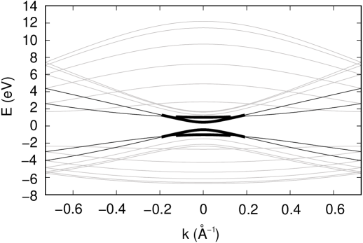
Figure 3: Results of the proposed optimization of the tight-binding method in the case of a $(10,0)$ nanotube. The thin black lines are the (doubly degenerate) bands obtained cross-sectioning the graphene dispersion relations along the segments closest to the two graphene degeneration points inside the considered rectangle and the thick black lines are the parts of these bands obtained taking the cross-sections only in the circular regions (with radius equal to $(5/6)\,|\vec{K}_{1}|$) centered around the two graphene degeneration points. The gray curves represent the nanotube dispersion relations that with our procedure we do not need to compute, if we are not interested in them.

Incidentally, we note that an alternative method to calculate only the most relevant nanotube energy bands could consist in taking the cross-sections of the graphene dispersion relations (along the parallel lines corresponding to the allowed wave vectors) in the hexagonal Brillouin zone of graphene (which evidently contains all and only the inequivalent graphene wave vectors), instead of inside the considered rectangular region. In this case the positions of the maximum and minimum points are well known ($\vec{K}$ and $\vec{K}^{\prime}$ are at the vertices of the hexagon) and thus the regions of interest are clearly located. Following this method, however, in order to fold the computed cross-sections into the nanotube Brillouin zone (the segment of the $\hat{T}$ axis characterized by $-\pi/T<k_{T}\leq\pi/T$), it is not sufficient to consider the $k_{T}$ component along $\hat{T}$ of the graphene wave vector (the absolute value of this component can be greater than $\pi/T$), but we also need to find the nanotube wave vector equivalent to $k_{T}$ inside the nanotube Brillouin zone. Moreover, since the graphene degeneration points are on the boundary of the sectioned hexagonal region, in order to obtain the nanotube bands around their minima and maxima we have to properly join the results computed cross-sectioning the graphene dispersion relations near the six vertices (each of which gives only parts of the desired bands); this strongly increases the algorithmic complexity of the involved computations.

IV Conclusion

We have proposed an alternative choice of unit vectors for the graphene sheet which, once rolled up, forms a carbon nanotube. These vectors, which depend on the considered nanotube, are closely related to the rectangular region of the graphene reciprocal space where the zone-folding method is most easily applied, and allow us to better understand the relation between this rectangular area and the overall reciprocal space. In particular, we have shown that our choice of unit vectors can be exploited to find, from any graphene wave vector, the equivalent wave vector inside the rectangular region and can therefore be useful whenever the zone-folding technique is applied to obtain the physical properties of the carbon nanotube from those of graphene. As an example, we have presented an application to the optimization of the tight-binding calculation of the carbon nanotube energy dispersion relations, with a significant reduction of computational times.

Supplementary Information

In the following, we provide a demonstration of the fact that the rectangular region of the graphene reciprocal space defined by the vectors $N\vec{K}_{1}$ and $\vec{K}_{2}$ contains all and only the inequivalent graphene wave vectors and can therefore be considered as a primitive unit cell of the graphene reciprocal lattice.
This rectangular region has an area

$$N\frac{2\pi}{L}\cdot\frac{2\pi}{T}=\frac{2L^{2}}{a^{2}d_{R}}\frac{2\pi}{L}2\pi\frac{d_{R}}{\sqrt{3}L}=\frac{8\pi^{2}}{\sqrt{3}a^{2}}\quad,$$ (23)

that is equal to $|\vec{b}_{1}\times\vec{b}_{2}|$ and thus to the area of the graphene Brillouin zone. Thus our assertion is automatically verified if we demonstrate that such a region does not contain two distinct but equivalent (i.e. differing only for a linear combination with integer coefficients of $\vec{b}_{1}$ and $\vec{b}_{2}$) graphene wave vectors $\vec{k}=k_{C}\hat{C}_{h}+k_{T}\hat{T}$ and $\vec{k}^{\prime}=\vec{k}+N_{1}\vec{b}_{1}+N_{2}\vec{b}_{2}=k^{\prime}_{C}\hat{C}_{h}+k^{\prime}_{T}\hat{T}$ (with $N_{1}$ and $N_{2}$ two integer numbers).
Indeed, if $\vec{k}$ is inside the rectangular region, we have that

$$\left\{\begin{array}[]{l}\displaystyle 0\leq k_{C}<N\frac{2\pi}{L}\\ \\[-10.0pt] \displaystyle-\frac{\pi}{T}<k_{T}\leq\frac{\pi}{T}\\ \end{array}\right.\quad\textrm{and therefore}\quad\left\{\begin{array}[]{l}\displaystyle-N\frac{2\pi}{L}<-k_{C}\leq 0\\ \\[-10.0pt] \displaystyle-\frac{\pi}{T}\leq-k_{T}<\frac{\pi}{T}\\ \end{array}\right.\quad.$$ (24)

If also $\vec{k}^{\prime}$ is inside the rectangular region, we have that

$$\left\{\begin{array}[]{l}\displaystyle 0\leq k^{\prime}_{C}<N\frac{2\pi}{L}\\ \\[-10.0pt] \displaystyle-\frac{\pi}{T}<k^{\prime}_{T}\leq\frac{\pi}{T}\\ \end{array}\right.\quad\textrm{or equivalently}\quad\left\{\begin{array}[]{l}\displaystyle 0\leq k_{C}+N_{1}b_{1_{C}}+N_{2}b_{2_{C}}<N\frac{2\pi}{L}\\ \\[-10.0pt] \displaystyle-\frac{\pi}{T}<k_{T}+N_{1}b_{1_{T}}+N_{2}b_{2_{T}}\leq\frac{\pi}{T}\\ \end{array}\right.\quad.$$ (25)

From these last relations, exploiting the inequalities for $-k_{C}$ and $-k_{T}$, we have that

$$\left\{\begin{array}[]{l}\displaystyle-N\frac{2\pi}{L}<-k_{C}\leq N_{1}b_{1_{C}}+N_{2}b_{2_{C}}<-k_{C}+N\frac{2\pi}{L}\leq N\frac{2\pi}{L}\\ \\[-10.0pt] \displaystyle-\frac{2\pi}{T}\leq-k_{T}-\frac{\pi}{T}<N_{1}b_{1_{T}}+N_{2}b_{2_{T}}\leq-k_{T}+\frac{\pi}{T}<\frac{2\pi}{T}\\ \end{array}\right.\quad.$$ (26)

This implies that that

$$\left\{\begin{array}[]{l}\displaystyle-N\frac{2\pi}{L}<N_{1}b_{1_{C}}+N_{2}b_{2_{C}}<N\frac{2\pi}{L}\\ \\[-10.0pt] \displaystyle-\frac{2\pi}{T}<N_{1}b_{1_{T}}+N_{2}b_{2_{T}}<\frac{2\pi}{T}\\ \end{array}\right.\quad\textrm{and thus}\quad\left\{\begin{array}[]{l}\displaystyle|N_{1}b_{1_{C}}+N_{2}b_{2_{C}}|<N\frac{2\pi}{L}\\ \\[-10.0pt] \displaystyle|N_{1}b_{1_{T}}+N_{2}b_{2_{T}}|<\frac{2\pi}{T}\\ \end{array}\right.\quad.$$ (27)

Substituting into (27) the values of the components of $\vec{b}_{1}$ and $\vec{b}_{2}$ along $\hat{C}_{h}$ and $\hat{T}$, we have that

$$\left\{\begin{array}[]{l}|N_{1}n+N_{2}m|<N\\ |N_{1}t_{1}+N_{2}t_{2}|<1\\ \end{array}\right.\quad.$$ (28)

Being $N_{1}t_{1}+N_{2}t_{2}$ an integer number, the second inequality is equivalent to the relation $N_{1}t_{1}+N_{2}t_{2}=0$. Since $N_{1}$ and $N_{2}$ have to be integer numbers, and $t_{1}$ and $t_{2}$ are two relative prime integer numbers, this identity is satisfied only if $N_{1}=\ell t_{2}$ and $N_{2}=-\ell t_{1}$, with $\ell$ an integer number. With these values of $N_{1}$ and $N_{2}$, we have that $N_{1}n+N_{2}m=\ell(t_{2}n-t_{1}m)=-\ell N$ (as we have seen, $mt_{1}-nt_{2}=N$). Thus the first inequality of (28) becomes $|\ell|N<N$ and is satisfied only if $\ell=0$. This means that $N_{1}=\ell t_{2}=0$ and $N_{2}=-\ell t_{1}=0$ and thus $\vec{k}^{\prime}$ is identical to $\vec{k}$, as we wanted to prove.

References

- (1) Meyyappan M. Carbon Nanotubes: Science and Applications. Boca Raton, Florida: CRC Press; 2005.
- (2) Ajayan PM, Zhou OZ. Applications of Carbon Nanotubes. In: Dresselhaus MS, Dresselhaus G, Avouris Ph, editors. Carbon Nanotubes: Synthesis, Structure, Properties, and Applications (Topics in Applied Physics, vol 80), Berlin: Springer, 2000; p. 391–425.
- (3) Hamada N, Sawada S, Oshiyama A. New One-dimensional Conductors: Graphitic Microtubules. Phys Rev Lett 1992; 68(10), 1579–1581.
- (4) Mintmire JW, Dunlap BI, White CT. Are Fullerene Tubules Metallic?. Phys Rev Lett 1992; 68(5), 631–634.
- (5) Saito R, Fujita M, Dresselhaus G, Dresselhaus MS. Electronic structure of chiral graphene tubules. Appl Phys Lett 1992; 60(18), 2204–2206.
- (6) Saito R, Dresselhaus G, Dresselhaus MS. Physical Properties of Carbon Nanotubes. London: Imperial College Press; 1998.
- (7) Reich S, Thomsen C, Maultzsch J. Carbon Nanotubes. Weinheim: Wiley-VCH; 2004.
- (8) Ashcroft NW, Mermin ND. Solid State Physics. London: Brooks/Cole Thomson Learning; 1976.
- (9) Reich S, Maultzsch J, Thomsen C, Ordejón P. Tight-binding description of graphene. Phys Rev B 2002; 66, 035412-1–5.