Self field of ac current reveals voltage–current law in type-II superconductors

Abstract

The distribution of ac magnetic fields in a thin superconducting strip is calculated when an ac current is applied to the sample. The edge barrier of the strip to flux penetration and exit is taken into account. The obtained formulas provide a basis to extract voltage-current characteristics in the bulk and at the edges of superconductors from the measured ac magnetic fields. Based on these results, we explain the spatial and temperature dependences of the profiles of the ac magnetic field measured in a Bi₂Sr₂CaCu₂O₈ strip [D.T. Fuchs et al., Nature 391, 373 (1998)].

I Introduction

Recently a novel experimental approach for mapping the distribution of the transport current across a flat superconducting sample was developed. 1 ; 2 In this technique an array of microscopic Hall sensors is attached directly to the sample and the perpendicular component of the magnetic self-field generated by an ac transport current is measured at various locations across the sample. Inverting the Biot-Savart law, the distribution of the transport current across the sample can be obtained from the measured self field. It was found that in contrast to the common assumptions the transport-current distribution is highly nonuniform and varies significantly as a function of temperature $T$, the applied magnetic field $H_{a}$, and the phase of the vortex matter, Fig. 1. Surprisingly, over a wide range of the $H$-$T$ phase diagram the current flows predominantly at the edges of the sample due to significant surface barriers both in high-$T_{c}$ and clean low-$T_{c}$ superconductors. 1 ; 2 ; 3 In this situation the velocity of the vortex lattice is determined by the rate of the vortex activation over the surface barrier rather than by the bulk vortex pinning. At lower temperatures bulk vortex dynamics takes over, resulting in redistribution of the transport current; see Fig. 1. So far, however, the experimental data thus obtained were not used for quantitative study of vortex dynamics due to the absence of a detailed theoretical description.

In this paper we develop such a description. It provides the basis for the extraction of various voltage-current characteristics in the bulk and at the edges of superconductors. In Sec. II we give general formulas for the ac magnetic fields and currents, while in Secs. III-V three simple models are considered which shed light on the data presented in Fig. 1. Combinations of these models (or of more complicated models developed on the basis of the general equations of Sec. II) enable one to analyze various experimental situations in different superconductors. The obtained results show that the self-field method can be a useful tool for determination of the voltage–current characteristics of superconductors. This development supplements the usual transport measurements and thus opens novel possibilities for a quantitative investigation of vortex dynamics.

Figure 1: Top: The temperature dependence of the in-phase part of the first harmonic of the ac self field measured by an array of 7 Hall probes at the surface of a Bi₂Sr₂CaCu₂O₈ strip carrying an ac current of 4 mA amplitude in a constant applied dc field of 1000 G. Bottom: The temperature dependence of the second harmonic of the ac magnetic field measured by one of the sensors at 10 mA ac current at 1000 G. Shown are also the characteristic temperatures $T_{d}$, $T_{sb}$, $T_{x}$. All the data from Ref. 2, . The inset shows the geometry of the experiment and the positions of the sensors.

II General formulas for AC magnetic field and current

II.1 Edge barrier

Consider an infinitely long thin superconducting strip of width $2w$ and thickness $d\ll w$, filling the space $|x|\leq w$, $|y|<\infty$, $|z|\leq d/2$. Let the strip be in a constant and uniform external magnetic field $H_{a}$ directed along the $z$ axis, and let an ac current $I_{a}=I_{a0}\sin\omega t$ of frequency $\omega$ and of magnitude $I_{a0}$ be applied to the sample. The current–voltage dependence for the superconducting strip in the bulk is implied to have the standard form $E=\rho(|j|)j$, with resistivity $\rho$ being a nonlinear function of the current density $j$: At small current densities, $|j|<j_{c}$, the resistivity $\rho$ (and thus the electric field $E$) is practically equal to zero; near the critical current density $j_{c}$ (i.e., at $|j|\approx j_{c}$) the resistivity sharply increases, and it reaches a constant value $\rho_{\rm ff}$ independent of $j$ in the flux-flow regime at $|j|\gg j_{c}$.

In the narrow regions of the strip near its right and left edges $x=\pm w$ where the barrier for flux penetration into the strip or exit from it occurs, we shall use the current–voltage laws: $E=R_{r}I_{r}$, $E=R_{l}I_{l}$ where $I_{r}$ and $I_{l}$ are the currents that flow in these edge regions while $R_{r}$ and $R_{l}$ are the appropriate resistances per unit length in $y$. In other words, we model the small edge regions of the strip as “wires” with the resistances $R_{r}$ and $R_{l}$. Since the edge barrier is generally different for flux entrance into the sample and for flux exit from it, bkv these resistances are generally different, too. When $I_{a}>0$, the vortices enter the strip at $x=-w$ and exits from it at $x=w$, i.e., one has $R_{l}=R_{en}$ and $R_{r}=R_{ex}$, while at $I_{a}<0$ we arrive at the opposite relations: $R_{l}=R_{ex}$ and $R_{r}=R_{en}$. In general, $R_{ex}$ and $R_{en}$ are nonlinear functions of the currents flowing in the appropriate edge regions. bkv

We may estimate the radius of the two edge wires from the following arguments. For a strip in a parallel magnetic field when $H_{a}$ is applied along the $x$ axis and is larger than the penetration field, the $z$-size of the region where the surface currents flow is less than the London penetration depth $\lambda$. Clem It is generally believed that under condition $\lambda\ll d$, which usually holds for single crystals of high-$T_{c}$ superconductors, this is also true in the considered case of a perpendicular magnetic field ($H_{a}\parallel z$) if $H_{a}$ is higher than the lower critical field $H_{c1}$. In other words, one might expect that the width of the edge wires is less or of the order of $\lambda$. However, simple considerations show that this is not the case since this assumption leads to a contradiction at least for not-too-large ratio $H_{a}/H_{c1}$. Indeed, consider the situation when flux line pinning is negligible. If the edge currents flew only at $w\geq|x|\geq w-\lambda$, they would generate both $H_{z}$ and $H_{x}$ at least in the region $w\geq|x|\geq w-d$. This means that the flux lines are curved at such $x$. But without pinning and currents the curved flux lines cannot be in equilibrium. Thus, we conclude that in a strip in a perpendicular magnetic field the edge currents flow in the whole region $w-|x|\leq d$ and probably have a complicated distribution over $x$ and $z$ there. With this in mind we shall assume below that the width of the edge wires is of the order of $d$. Note that for $H_{a}$ of the order of the lower critical field $H_{c1}$ this assumption agrees with the known result for the width of the geometrical barrier. Z

II.2 Simple case

We now consider the magnetic field $H_{z}(x,t)$ generated by the ac current $I_{a}=I_{a0}\sin\omega t$. In particular, we calculate the first and the second harmonics of the ac magnetic field $H_{z}$:

$$H_{z}^{(1)}(x)=\frac{2}{T}\int_{0}^{T}H_{z}(x,t)\sin{\omega t}dt,$$ (1)

$$H_{z}^{(2)}(x)=\frac{2}{T}\int_{0}^{T}H_{z}(x,t)\cos{2\omega t}dt,$$ (2)

where $T=2\pi/\omega$ is the period of the oscillating ac current. (When the inductance of the strip is negligible, it follows from symmetry considerations that the first harmonic proportional to $\cos\omega t$ and the second harmonic proportional to $\sin 2\omega t$ are equal to zero.)

The total current $I_{a}$ flowing in the strip at time $t$ splits into the bulk current $I_{b}$ and the edge current $I_{e}$,

$$I_{a}=I_{b}+I_{e},$$ (3)

where $I_{e}$ consists of the left ($I_{l}$) and right ($I_{r}$) parts,

$$I_{e}=I_{l}+I_{r}.$$ (4)

If the frequency $\omega$ is not too large, the current distribution over the cross-section of the sample is uniform, and hence the sheet current in the strip $J(x)$ (i.e., the current density integrated over the thickness $d$ of the strip) is independent of $x$,

$$J(x)={I_{b}\over 2w}\,.$$ (5)

In this case we immediately obtain

$$I_{e}=I_{a}{R_{b}\over R_{b}+R_{e}}\,,\ \ \ I_{b}=I_{a}{R_{e}\over R_{b}+R_{e}}\,,$$ (6)

where $R_{b}=\rho(J/d)/2wd$ and

$$R_{e}={R_{l}R_{r}\over R_{l}+R_{r}}={R_{en}R_{ex}\over R_{en}+R_{ex}}\,.$$ (7)

As to $I_{l}$ and $I_{r}$, one finds

$$I_{l}=I_{e}{R_{r}\over R_{l}+R_{r}}\,,\ \ \ I_{r}=I_{e}{R_{l}\over R_{l}+R_{r}}\,,$$ (8)

with

$$R_{l}=R_{en}\,,\ \ \ R_{r}=R_{ex}\ \ \ \ {\rm for}\ I_{a}>0,$$ (9)

and

$$R_{l}=R_{ex}\,,\ \ \ R_{r}=R_{en}\ \ \ \ {\rm for}\ I_{a}<0.$$ (10)

As was mentioned above, $R_{b}$, $R_{en}$ and $R_{ex}$ are generally nonlinear functions of $J=I_{b}/2w$ and of the currents $I_{en}$ and $I_{ex}$, i.e., $R_{b}=R_{b}(I_{b})$, $R_{en}=R_{en}(I_{en})$ and $R_{ex}=R_{ex}(I_{ex})$, where $I_{en}=I_{l}$, $I_{ex}=I_{r}$ for $I_{a}>0$, and $I_{en}=I_{r}$, $I_{ex}=I_{l}$ for $I_{a}<0$. Therefore, formulas (6) - (8) are in fact equations for $I_{b}$, $I_{l}$ and $I_{r}$,

$$I_{l}\!=\!I_{a}{R_{r}(I_{r})R_{b}(I_{b})\over[R_{l}(I_{l})+R_{r}(I_{r})]R_{b}(I_{b})+R_{r}(I_{r})R_{l}(I_{l})},~{}$$ (11)

$$I_{r}\!=\!I_{a}{R_{l}(I_{l})R_{b}(I_{b})\over[R_{l}(I_{l})+R_{r}(I_{r})]R_{b}(I_{b})+R_{r}(I_{r})R_{l}(I_{l})},~{}$$ (12)

$$I_{b}\!=\!I_{a}{R_{r}(I_{r})R_{l}(I_{l})\over[R_{l}(I_{l})\!+\!R_{r}(I_{r})]R_{b}(I_{b})\!+\!R_{r}(I_{r})R_{l}(I_{l})}.~{}$$ (13)

On determining $I_{l}$, $I_{r}$, and $I_{b}$ from this set of equations, one can calculate $H_{z}(x,t)$ as sum of the fields of the wires and of the spatially uniform sheet current $J$,

$$H_{z}(x,t)={1\over 2\pi}\left({I_{b}\over 2w}\ln\Big{|}{w-x\over w+x}\Big{|}+{I_{r}\over w-x}-{I_{l}\over w+x}\right).$$ (14)

This formula together with Eqs. (11)-(13) gives $H_{z}$ as a function of $x$ and $I_{a}$, $H_{z}=H_{z}(x,I_{a})$. Expressing the time $t$ in Eqs. (1), (2) via $I_{a}$, $\sin\omega t=I_{a}/I_{a0}=\tilde{I}_{a}$, we arrive at

$$H_{z}^{(1)}(x)=\frac{4}{\pi}\int_{0}^{1}H_{z}(x,\tilde{I}_{a}){\tilde{I}_{a}d\tilde{I}_{a}\over(1-\tilde{I}_{a}^{2})^{1/2}},\ \$$ (15)

$$H_{z}^{(2)}(x)\!=\!\frac{2}{\pi}\!\int_{0}^{1}\!\![H_{z}(x,\tilde{I}_{a}\!)\!+\!H_{z}(x,-\tilde{I}_{a}\!)]{(1-2\tilde{I}_{a}^{2})d\tilde{I}_{a}\over(1-\tilde{I}_{a}^{2})^{1/2}}.$$ (16)

Note that $H_{z}(x,-\tilde{I}_{a})\neq-H_{z}(x,\tilde{I}_{a})$ only if $R_{en}\neq R_{ex}$. Hence, the second harmonic $H_{z}^{(2)}(x)$ appears only when an edge barrier exists, and when this barrier leads to an asymmetry with $I_{l}\neq I_{r}$. Using formulas (3), (4), (14), expressions (15), (16) can be also rewritten in the form

$$\!\!H_{z}^{(1)}\!(x)\!\!\! = \!\!\!{1\over 4\pi w}\!\!\left(\![I_{a0}\!-\!I_{e}^{(1)}]\ln\Big{|}{w\!-\!x\over w\!+\!x}\Big{|}\!+\!I_{e}^{(1)}\!\!{2wx\over w^{2}\!-\!x^{2}}\!\!\right)\!\!,~{}~{}$$ (17)

$$\!\!H_{z}^{(2)}\!(x)\!\!\! = \!\!\!{w\over 2\pi(\!w^{2}\!-\!x^{2}\!)}\,\Delta I_{e}^{(2)},$$ (18)

where $I_{e}^{(1)}$ is the first harmonic of $I_{e}$, while $\Delta I_{e}^{(2)}$ is the second harmonic of $I_{r}-I_{l}$,

$$I_{e}^{(1)}\!=\frac{4}{\pi}\int_{0}^{1}\!\![I_{r}(\tilde{I}_{a}\!)\!+\!I_{l}(\tilde{I}_{a}\!)]{\tilde{I}_{a}d\tilde{I}_{a}\over(1-\tilde{I}_{a}^{2})^{1/2}},$$

$$\Delta I_{e}^{(2)}\!=\frac{4}{\pi}\int_{0}^{1}\!\![I_{r}(\tilde{I}_{a}\!)\!-\!I_{l}(\tilde{I}_{a}\!)]{(1-2\tilde{I}_{a}^{2})d\tilde{I}_{a}\over(1-\tilde{I}_{a}^{2})^{1/2}}.$$

II.3 General case

Formulas (5)-(13) have been obtained under the assumption that the resistances are much larger than $\mu_{0}\omega$ (quasistatic approximation),

$$R_{l},\ R_{r},\ R_{b}\ \gg\mu_{0}\omega,$$ (19)

where $R_{b}=\rho(J/d)/2wd$. Under this assumption one can neglect the inductance of the sample, which is of the order of $\mu_{0}$ (per unit length).ll Besides this, when $R_{b}\gg\mu_{0}\omega$, the two-dimensional penetration depth eh1 ; eh2 $\Lambda=\rho_{\rm ff}/\mu_{0}\omega d$ of the ac field in the Ohmic regime is considerably larger than the width $2w$ of the strip,

$${\Lambda\over 2w}={{\rm R}_{\rm ff}\over\mu_{0}\omega}\gg 1,$$ (20)

and hence, one may expect that the current distribution over the cross section of the sample is indeed uniform. Since the resistances $R_{l}$, $R_{r}$, $R_{b}$ decrease with decreasing temperature $T$, the assumption (19) is true for not too low temperatures. We now address the general case when conditions (19) are not necessarily fulfilled. c1

Let $E_{a}$ be the voltage drop (per unit length) which just generates the current $I_{a}$. We now consider not only the edge regions but formally also the whole strip as a set of parallel wires. Then, we arrive at the following set of equations for the left and right edge wires and for the wires of width $dx$ at points $x$ ($-w<x<w$):

$$E_{a}\!\!\! = \!\!\!R_{l}I_{l}\!+\!L_{w}\dot{I}_{l}\!+\!L_{lr}\dot{I}_{r}\!+\!\int_{-w}^{w}\!\!\!\!\!dx\dot{J}(x,t)L_{xl},$$ (21)

$$E_{a}\!\!\! = \!\!\!R_{r}I_{r}\!+\!L_{w}\dot{I}_{r}\!+\!L_{lr}\dot{I}_{l}\!+\!\int_{-w}^{w}\!\!\!\!\!dx\dot{J}(x,t)L_{xr},$$ (22)

$$E_{a}\!\!\! = \!\!\!\rho_{x}J(x)\!+\!L_{xl}\dot{I}_{l}\!+\!L_{xr}\dot{I}_{r}\!+\!\!\int_{-w}^{w}\!\!\!\!\!dx^{\prime}\dot{J}(x^{\prime}\!,t)L_{xx^{\prime}},$$ (23)

$$I_{a}\!\! = \!\!I_{l}+I_{r}+I_{b},$$ (24)

where $\rho_{x}\equiv\rho[J(x)/d]/d$ is the sheet resistance,

$$I_{b}=\int_{-w}^{w}\!\!\!\!\!dxJ(x,t),$$ (25)

the dot over currents means the time derivative, $L_{xx^{\prime}}=(\mu_{0}/2\pi)\ln(l/|x-x^{\prime}|)$ is the mutual inductance per unit length of two parallel wires of length $l$ located at points $x$ and $x^{\prime}$, ll $L_{xl}=(\mu_{0}/2\pi)\ln(l/|x+w|)$ and $L_{xr}=(\mu_{0}/2\pi)\ln(l/|x-w|)$ give the mutual inductances of the edge wires and that located at $x$, $L_{lr}=(\mu_{0}/2\pi)\ln(l/2w)$ is the mutual inductance of the two edge wires, and $L_{w}=(\mu_{0}/2\pi)[\ln(l/r)+1/4]$ is the self inductance of the edge wires. Here we have assumed that both edge wires have the characteristic radius $r\sim d/2$. The magnetic field $H_{z}(x,t)$ is given by the Biot-Savart law

$$H_{z}(x,t)=\!{1\over 2\pi}\!\left(\!{I_{r}\over w-x}-\!{I_{l}\over w+x}+\!\int_{-w}^{w}\!\!\!{J(x^{\prime},t)\,dx^{\prime}\over x^{\prime}-x}\right)\!.$$ (26)

Note that under conditions (19), one may keep only the first terms on the right hand sides of Eqs. (21)-(23) (omitting all time derivatives) and replace formula (25) by Eq. (5) (since the skin effect is absent). After this simplification, equations (21)- (24) and (26) are equivalent to formulas (6) - (14).

In some region above temperature $T_{d}$ shown in Fig. 1, one has $R_{b}\gg R_{e}$. Thus, a situation is possible in which $R_{b}\gg\mu_{0}\omega>R_{e}$, and the skin effect is negligible, but one cannot omit completely the terms with the inductances in Eq. (21)-(23). In this context, it is useful to consider the case when the only assumption is the uniform distribution of the sheet current over $x$, i.e., the fulfilment of Eq. (5). Under this assumption Eq. (21)- (24) reduce to a form which describes three parallel connected conductors with inductive coupling:

$$E_{a}\!\!\! = \!\!\!R_{l}I_{l}\!+\!L_{w}\dot{I}_{l}\!+\!L_{lr}\dot{I}_{r}\!+\!L_{wb}\dot{I}_{b},$$ (27)

$$E_{a}\!\!\! = \!\!\!R_{r}I_{r}\!+\!L_{w}\dot{I}_{r}\!+\!L_{lr}\dot{I}_{l}\!+\!\!L_{wb}\dot{I}_{b},$$ (28)

$$E_{a}\!\!\! = \!\!\!R_{b}I_{b}\!+\!L_{wb}\dot{I}_{l}\!+\!L_{wb}\dot{I}_{r}\!+\!\!L_{b}\dot{I}_{b},$$ (29)

$$I_{a}\!\! = \!\!I_{l}+I_{r}+I_{b},$$ (30)

where $R_{b}=\rho(j)/2wd$ with $j=I_{b}/2wd$, $L_{b}=(\mu_{0}/2\pi)[\ln(l/2w)+3/2]$ is the inductance of the strip for uniform current distribution in it, and $L_{wb}=(\mu_{0}/2\pi)[\ln(l/2w)+1]$ is the mutual inductance of the strip and one of the edge wires. In this case Eq. (26) transforms into expression (14), and formulas (17), (18) are valid.

Equations (21)-(24) generalize the known equation for a strip with time-dependent current, eh1 ; eh2 which follows from Eq. (23) if one omits the edge-wire terms with $\dot{I}_{l}$ and $\dot{I}_{r}$. Thus, the numerical procedure elaborated in Refs. eh1, , eh2, can be applied to solve Eqs. (21)- (24) in the general case. However, in this paper we shall confine our analysis to simple models which are sufficient to understand the main features of the experimental results obtained in Refs. 1, ; 2, ; 3, .

III Ohmic model

We begin our analysis with the simplified symmetric Ohmic model in which $R_{en}=R_{ex}=2R_{e}$, and these resistances are independent of the currents $I_{en}=I_{ex}$ but depend on temperature $T$. We shall use a temperature dependence that satisfies the following requirement: At $T=T_{c}$ when the edge barrier is absent, the resistances are proportional to $R_{b}$ with a geometrical factor that is the ratio of the cross-section area of the strip to the cross-section area of one of the edge wires. At lower temperatures we then take the conductance of the edge wires, $1/R_{en}$, $1/R_{ex}$, as a sum of this bulk contribution and the conductance caused by the edge barrier:

$${1\over R_{en}(T)}\!=\!{1\over R_{ex}(T)}\!=\!{1\over R_{0}(T)}\!+\!{1\over 2R_{e}^{0}}\!\left(\exp\!\!{{U_{e}(t)\over t}}-1\right)\!,$$ (31)

where $R_{0}(T)=(w/r)R_{b}(T)$, $R_{e}^{0}$ is some constant, $t\equiv T/T_{c}$, $T_{c}$ is the temperature of the superconducting transition, $U_{e}(t)$ is the dimensionless magnitude of the edge barrier (in units of $T_{c}$), and we shall imply a linear temperature dependence of this barrier, $U_{e}(T)=U_{e}(0)(1-t)$, with some constant $U_{e}(0)$. The function $R_{0}(T)$ just gives the resistance of one of the edge wires with the edge barrier neglected ($r\sim d/2$ is the characteristic radius of the edge wire), while the second term in Eq. (31) is the edge contribution described by an Arrhenius law. We have introduced the constant $-1$ in the brackets to take into account that this part of the conductance vanishes at $T_{c}$. Besides this, in this Ohmic model we use $j_{c}(T)=0$, and thus $R_{b}$ is independent of $J$ at all temperatures. For definiteness we take the temperature dependence of $R_{b}$ in the form of an Arrhenius law, too, $R_{b}(T)=\rho_{\rm ff}/2wd=R_{b}(T_{c})\exp[-U_{b}(0)(1-t)/t]$, but with the constant $U_{b}(0)$ smaller than $U_{e}(0)$. The requirement $U_{b}(0)<U_{e}(0)$ emphasizes that with decreasing temperature the main contribution to the conductance of the edge wires results from the edge barrier. In the discussion below, we shall imply parameters that correspond to the experimental values: 1 ; 2 $I_{a0}=4$ mA, $w=75\ \mu$m, $d=10\ \mu$m, $2w/d=15\ (\approx w/r)$, $l=1.5\$mm, $T_{c}=88$ K, $\omega/2\pi=73$ Hz, $R_{b}(T_{c})\approx 6.7\ \Omega/$cm, yielding the large value $\Lambda/w=2.32\cdot 10^{6}$ for the two dimensional penetration depth at $T=T_{c}$. For definiteness, in the construction of figures we shall also take $R_{e}^{0}=R_{0}(T_{c})$. As to $U_{e}(0)$ and $U_{b}(0)$, we chose them so that one can reproduce the characteristic temperatures $T_{d}$ and $T_{sb}$ marked in Fig. 1.

Within this simplified model, one has $H_{z}^{(1)}(x)=H_{z}(x,t)/\sin\omega t$ and $H_{z}^{(2)}(x)=0$, where under conditions (19) (at sufficiently high temperatures) $H_{z}(x,t)$ is given by Eq. (14), while $I_{e}(=2I_{l}=2I_{r})$ and $I_{b}$ are described by Eqs. (6). Thus, we obtain

$$H_{z}^{(1)}\!(x)\!\!=\!\!{I_{a0}\over 4\pi w}\!\!\left(\!{R_{e}\over R_{e}\!+\!R_{b}}\ln\!\Big{|}{w\!-\!x\over w\!+\!x}\Big{|}\!+\!{R_{b}\over R_{e}\!+\!R_{b}}{2wx\over w^{2}\!-\!x^{2}}\!\right)\!\!.~{}$$ (32)

With decreasing temperature when the inequality $R_{e}<\mu_{0}\omega$ becomes valid, it is necessary to take into account the inductances of the strip and of the edge wires. In this case Eqs. (27)-(30) reduce to a set of linear equations (the time derivatives are replaced by the factor $i\omega$), and after simple calculations we find

$$2I_{l}=2I_{r}=I_{e}=I_{a}{\tilde{z}_{b}\over\tilde{z}_{b}+\tilde{z}_{e}}\,,\ \ \ I_{b}=I_{a}{\tilde{z}_{e}\over\tilde{z}_{b}+\tilde{z}_{e}}\,,$$ (33)

where $\tilde{z}_{b}$ and $\tilde{z}_{e}$ are the “effective impedances” of the strip and of the two edge wires,

$$\tilde{z}_{b}\!\!\! = \!\!R_{b}+i\omega(L_{b}-L_{wb})=R_{b}+i\omega{\mu_{0}\over 4\pi}\,,$$ (34)

$$\tilde{z}_{e}\!\!\! = \!\!R_{e}\!+\!i\omega\!\left({L_{w}\over 2}+\!{L_{lr}\over 2}-\!L_{wb}\right)$$ (35)

$$\ \ \ =R_{e}+i\omega{\mu_{0}\over 4\pi}\left(\ln\!{2w\over r}\,-{7\over 4}\right).$$

Note that even though the various inductances calculated per unit length of the strip depend logarithmically on its length $l$, the resulting effective impedances $\tilde{z}_{b}$, $\tilde{z}_{e}$ (per unit length) are independent of $l$. Inserting expressions (33) in formula (14), one obtains $H_{z}^{(1)}(x)$. In other words, down to the temperature $T_{d}$ defined in the Ohmic model by $R_{b}(T_{d})\sim\mu_{0}\omega$, the first harmonic is described by formula (32) in which $R_{b}$ and $R_{e}$ are simply replaced by $\tilde{z}_{b}$ and $\tilde{z}_{e}$. The real part of this expression gives the harmonic which is in-phase with $I_{a}$, i.e., proportional to $\sin\omega t$ like $I_{a}(t)$, while the imaginary part corresponds to the out-of-phase signal proportional to $\cos\omega t$.

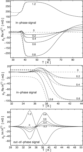
Figure 2: The temperature dependence of the first harmonic of the ac self field which is in-phase with the applied current, Re$H_{z}^{(1)}$, (top) and out-of-phase with it, Im$H_{z}^{(1)}$, (bottom) at positions $-x/w=1.2$, 0.8, 0.6, 0.4, 0.2, 0 on the surface of a long thin strip of width $2w$. The applied ac current is $I_{a}=I_{a0}\sin\omega t$. Results within the symmetric Ohmic model with $R_{en}=R_{ex}$ for $U_{e}(0)=21$, $U_{b}(0)=12$, $R_{b}(T_{c})=6.7\ \Omega/$cm, $w/r=15$, $R_{e}^{0}=15R_{b}(T_{c})$, $\omega/2\pi=73$ Hz, $T_{c}=88$ K, $w=75\ \mu$m, $I_{a0}=4$ mA. The dashed lines are the analytical results, Eq. (38), while the solid lines are numerical results from Eqs. (21)-(26) allowing for the skin effect. The solid and dashed lines coincide at $T>42$ K, see the enlarged plot (middle). Only numerical results are shown for Im$H_{z}^{(1)}$ (bottom) since the analytical results, Eq. (38), neglect the skin effect and thus are applicable only at $T>42$ K. Note the different scales of the $T$ axis for the different plots.

In Fig. 2 we show the temperature dependence of Re$H_{z}^{(1)}$ and Im$H_{z}^{(1)}$ for discrete values of $x$ similar to the locations of Hall sensors in the experiment. 1 ; 2 We first discuss the temperature dependence of the in-phase signal Re$H_{z}^{(1)}$. At temperatures near $T_{c}$, the bulk current $I_{b}$ exceeds $I_{e}$ since $R_{b}(T_{c})<R_{e}(T_{c})$, and one has an $H_{z}(x)$ that is characteristic of the normal state of the superconductor [the first term in Eq. (32) dominates], see Fig. 3. But the ratio of the currents $I_{e}$ and $I_{b}$ changes with temperature. The role of the edge current increases with decreasing $T$ since $U_{b}(0)<U_{e}(0)$, and at a temperature $T=T_{sb}\approx 69$ K defined by $R_{e}(T_{sb})=R_{b}(T_{sb})$ one has $I_{b}=I_{e}$, and the contributions of $I_{b}$ and $I_{e}$ to $H_{z}$ practically compensate each other for $x$ inside the strip. With further decrease of $T$, the $x$-dependence of $H_{z}$ is mainly determined by the edge current [i.e., by the second term in Eq. (32)]. When the inductances begin to play a role at temperature $T_{x}\approx 46$ K defined by $R_{e}(T_{x})\sim\mu_{0}\omega$ [or more exactly, by Re$\tilde{z}_{e}(T_{x})\sim{\rm Im}\tilde{z}_{e}(T_{x})$], the impedance $\tilde{z}_{e}$ saturates while $\tilde{z}_{b}$ still decreases with decreasing $T$. As the temperature $T_{d}\approx 38$ K corresponding to $R_{b}(T_{d})\sim\mu_{0}\omega$ is approached, the contribution of $I_{b}$ to $H_{z}$ begins to increase again, and the ratio of the currents, $I_{b}/I_{e}$ tends to the constant $\ln(2w/r)-7/4$, which is determined by the ratio of the imaginary parts of $\tilde{z}_{e}$ and $\tilde{z}_{b}$. Of course, in reality at such temperatures the skin effect plays an important role, and Re$H_{z}^{(1)}$ tends to zero rather than to a profile determined by the above-mentioned ratio of the currents, see Fig. 2. As to the out-of-phase part of the first harmonic Im$H_{z}^{(1)}$, it appears only near the temperature $T_{x}$ at which the inductances begin to play a role, and it differs from zero when the real and imaginary parts of the effective impedances are comparable. At still lower temperatures when $R_{e}$ and $R_{b}$ become negligible as compared to the imaginary parts of $\tilde{z}_{e}$ and $\tilde{z}_{b}$, the out-of-phase signal vanishes again.

Figure 3: The in-phase components of the magnetic field and of the sheet-current profiles, $H_{z}^{(1)}(x)$ (solid lines) and $J(x)$ (dashed lines), for the symmetric Ohmic model ($\eta=0$) at temperatures $T=85$, $70$, $50$, $38$, and $30$ K, accounting for the skin effect which occurs at $T<42$ K, cf. Fig. 2. The parameters of the model are as in Fig. 2. The circles mark the positions of the Hall probes used in Fig. 2. Both $H_{z}^{(1)}$ and $J$ are in units of $I_{a0}/w$. The total current in the depicted half strip is thus 1/2, equal to the area under the dashed lines plus the (not shown) edge current at $x=w$.

We now present the results for the asymmetric case when $R_{ex}\neq R_{en}$. In this situation model (31) is generalized as follows:

$${1\over R_{ex}(T)}={1\over R_{0}(T)}+{1\over R_{ex}^{0}}\left(\exp\!{U_{e}(t)\over t}-1\right),$$

$${1\over R_{en}(T)}={1\over R_{0}(T)}+{1\over R_{en}^{0}}\left(\exp\!{U_{e}(t)\over t}-1\right),$$ (36)

where $R_{ex}^{0}(T)$, $R_{en}^{0}(T)$ are some constants, and $R_{0}(T)$ is the same as in Eq. (31). It is convenient to introduce the parameter

$$\eta\equiv{R_{ex}^{0}-R_{en}^{0}\over R_{ex}^{0}+R_{en}^{0}}$$ (37)

which characterizes the asymmetry of the edge barrier. Then, one has

$$R_{en}^{0}=2R_{e}^{0}/(1+\eta),\ \ \ R_{ex}^{0}=2R_{e}^{0}/(1-\eta),$$

where $R_{e}^{0}=R_{en}^{0}R_{ex}^{0}/(R_{en}^{0}+R_{ex}^{0})$. We emphasize that the constant $\eta$ defines the ratio $(R_{ex}-R_{en})/(R_{ex}+R_{en})$ at sufficiently low temperatures when the conductance $1/R_{0}$ is negligible in Eqs. (36), while at $T\to T_{c}$ the resistances $R_{en}$ and $R_{ex}$ tend to $R_{0}$, the resistance of the edge wires without barrier. In other words, formulas (36) describe both the asymmetry of the edge wires at low temperatures, and the disappearance of the asymmetry when the edge barrier vanishes. Note also that $R_{e}=R_{ex}R_{en}/(R_{ex}+R_{en})$ is not equal to $R_{e}^{0}$ but approaches it with decreasing temperature.

In this asymmetric case the first harmonic becomes:

$$H_{z}^{(1)}\!(x)\!=\!{I_{a0}\over 4\pi w}\!\left(\!{\tilde{z}_{e\eta}\over\tilde{z}_{e\eta}\!+\!\tilde{z}_{b}}\ln\Big{|}{w\!-\!x\over w\!+\!x}\Big{|}\!+\!{\tilde{z}_{b}\over\tilde{z}_{e\eta}\!+\!\tilde{z}_{b}}{2wx\over w^{2}\!-\!x^{2}}\!\right)\!\!,~{}$$ (38)

where

$$\tilde{z}_{e\eta} = \tilde{z}_{e}+{(R_{ex}-R_{en})^{2}\over 4(R_{ex}+R_{en})}{ip\,\over 1+ip}\,,$$ (39)

$\tilde{z}_{e}$, $\tilde{z}_{b}$ are given by formulas (34), (35), and

$$p\equiv{2\omega(L_{w}-L_{lr})\over R_{ex}+R_{en}}={\mu_{0}\omega\over\pi(R_{ex}+R_{en})}\left(\ln\!{2w\over r}+{1\over 4}\right).$$ (40)

This $p$ characterizes the relative contribution of the inductance of the edge wires to their effective impedance $\tilde{z}_{e}$. Analysis of formulas (38)-(40) shows that the parameter $\eta$ practically has no effect on $H_{z}^{(1)}$ within the considered Ohmic model, and hence the first harmonic in the asymmetric case, in fact, coincides with the harmonic in the symmetric case of $\eta=0$. However, for the case $\eta\neq 0$ the second harmonic $H_{z}^{(2)}$ appears. This $H_{z}^{(2)}(x)$, Eq. (18), is

$$H_{z}^{(2)}\!(x)\!\!=\!\!{2I_{a0}\over 3\pi^{2}}{w\over w^{2}\!-\!x^{2}}{(R_{ex}\!-\!R_{en})\over(R_{ex}\!+\!R_{en})}{\tilde{z}_{b}\over\tilde{z}_{b}+\tilde{z}_{e\eta}}{1\over 1+ip}.$$ (41)

The real part of this expression gives the harmonic proportional to $\cos 2\omega t$, and its imaginary part to $\sin 2\omega t$. In Fig. 4 we show the temperature dependence of $|H_{z}^{(2)}|$ at $x=0.7w$. At temperatures near $T_{x}$ introduced by Re$\tilde{z}_{e}(T_{x})\sim{\rm Im}\tilde{z}_{e}(T_{x})$, one has $p(T_{x})\sim 1$, the amplitude of the second harmonic begins to decrease with decreasing $T$ and becomes small even at temperatures above $T_{d}$ if $R_{b}(T_{x})\gg\mu_{0}\omega$. Of course, at temperatures when $R_{b}(T)\sim\mu_{0}\omega$, the second harmonic $H_{z}^{(2)}$ vanishes in any case due to the skin effect.

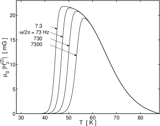
Figure 4: The temperature dependence of the magnitude of the second harmonic of the ac self field, $|H_{z}^{(2)}|$, at position $|x/w|=0.7$ on the surface of a long thin strip of width $2w$ with applied ac current $I_{a}=I_{a0}\sin\omega t$. Results within the Ohmic model, Eq. (41), for the same parameters as in Fig. 2 but with asymmetry $\eta=0.1$ and amplitude $I_{a0}=10$ mA (line at $\omega/2\pi=73$ Hz). The other lines are for different frequencies.

We emphasize that the formulas of this section are valid not only for the model dependences (31) or (36) used here but also for any functions $R_{b}(T)$, $R_{en}(T)$, $R_{ex}(T)$. Thus, one can obtain some information on these functions fitting the theoretical dependences of $H_{z}^{(1)}(T)$ and $H_{z}^{(2)}(T)$ to appropriate experimental data. Independent information on the functions $R_{b}(T)$, $R_{e}(T)$ for each specific sample can be also obtained from usual transport measurements. 4 Beside this, some data on this subject can be extracted from frequency dependences of $H_{z}^{(1)}(T)$ and $H_{z}^{(2)}(T)$ since these harmonics are functions of the combinations $(R_{b}/\mu_{0}\omega)$, $(R_{en}/\mu_{0}\omega)$, $(R_{ex}/\mu_{0}\omega)$. In the framework of our model (36), if one changes the frequency $\omega$ from $\omega_{1}$ to $\omega_{2}$, the temperature dependence of the first harmonic changes only near $T_{d}$, while the temperature dependence of the second harmonic changes in the vicinity of $T_{x}$ (the appropriate parts of these dependences shift to higher temperatures with increasing $\omega$), see, e.g., Fig. 4. The shifts of the temperatures $T_{d}$ and $T_{x}$ are

$$T_{d}(\omega_{2})-T_{d}(\omega_{1})\approx{T_{d}^{2}\over U_{b}(0)T_{c}}\ln\left({\omega_{2}\over\omega_{1}}\right),$$

$$T_{x}(\omega_{2})-T_{x}(\omega_{1})\approx{T_{x}^{2}\over U_{e}(0)T_{c}}\ln\left({\omega_{2}\over\omega_{1}}\right),$$ (42)

and they give information on $U_{b}(0)$ and $U_{e}(0)$.

We now briefly discuss the applicability of the considered temperature dependences of $R_{e}$ and $R_{b}$ to BSCCO samples. The experimental data on resistance of BSCCO strips obtained from usual transport measurements are well approximated by an Arrhenius law. P ; P1 ; B ; 4 In principle, parameters $U_{e}(0)$ and $R_{e}^{0}$ can be found from these data, while $U_{b}(0)$ can be estimated in similar experiments with wide samples.4 In particular, in Ref. 4, it was found that $U_{e}(0)\approx 12$ for the same crystal as in Fig. 2, and it was estimated that $U_{b}(0)\leq 8$. Both these values are noticeably less than those used in the construction of Figs. 2 and 4. The latter values were chosen such that one can reproduce the experimental $T_{d}$ and $T_{sb}$. In Figs. 2 and 4 we have also used the specific value of $R_{e}^{0}$, $R_{e}^{0}=R_{0}(T_{c})$. Other choices of the parameter $R_{e}^{0}$ enable one, in principle, to use a smaller value of $U_{e}(0)-U_{b}(0)$, but do not provide the coincidence of both $U_{e}(0)$ and $U_{b}(0)$ with their experimental values [in the Ohmic model the value of $U_{b}(0)\approx 12$ is fixed by the condition $R_{b}(T_{d})\approx\mu_{0}\omega$]. c Such disagreement seems to signal that the Ohmic model does not work in the whole interval from $T_{d}$ to $T_{c}$ for the BSCCO crystals.

Finally, we note two characteristic features of the Ohmic model studied here. First, if the magnetic field is measured in units of $I_{a0}/w$, the first and the second harmonics are independent of the amplitude $I_{a0}$ of the applied current. In particular, the characteristic temperatures $T_{d}$, $T_{bs}$, $T_{x}$ do not shift with a change of $I_{a0}$. This scaling property may be used in experiments to find the temperature regions where the Ohmic model is applicable. Second, the resistance of the strip, $R=R_{b}R_{e}/(R_{b}+R_{e})$ is also independent of $I_{a0}$ and can be used for the same aim as well.

IV Model of nonlinear $R_{e}(I_{e})$

The data of Ref. 3, obtained for different currents $I_{a0}$ show that at least for some superconductors $R_{e}$ cannot be considered as a quantity that is independent of $I_{e}$ for all temperatures. To get an insight into this problem, we shall now analyze a simple model of nonlinear dependence $R_{e}(I_{e})$ and show that this nonlinearity can provide an alternative description of the experimental temperature dependences of $H_{z}^{(1)}$ and $H_{z}^{(2)}$ near $T_{sb}$. In principle, this and a similar nonlinear model for $R_{b}(I_{b})$ near $T_{d}$ enable one to describe the experimental data on $H_{z}^{(1)}$ and $H_{z}^{(2)}$ with realistic values of $U_{e}(0)$ and $U_{b}(0)$.

We shall consider the following simple model dependences $R_{en}(I_{en})$ and $R_{ex}(I_{ex})$ for the flux entrance into the strip and the flux exit from it: When $I_{en}$ (or $I_{ex}$) exceeds the critical current $I_{en}^{c}$ ($I_{ex}^{c}$) for flux entrance (exit), the resistivity of the edge wire is the same as in the bulk of the strip, and hence the resistance of the edge wire $R_{en}(I_{en})$ [$R_{ex}(I_{ex})$] coincides with $R_{0}=(w/r)R_{b}$. At $I_{en}=I_{en}^{c}$ ($I_{ex}=I_{ex}^{c}$) the resistance sharply drops down to a value $R_{en}$ ($R_{ex}$) which is independent of the current $I_{en}$ ($I_{ex}$) for $I_{en}<I_{en}^{c}$ ($I_{en}<I_{en}^{c}$), i.e., one has

$$R_{en}(I_{en})=R_{0}\ \ {\rm for}\ \ I_{en}>I_{en}^{c},$$

$$R_{en}(I_{en})=R_{en}\ \ {\rm for}\ \ I_{en}<I_{en}^{c},$$ (43)

and

$$R_{ex}(I_{ex})=R_{0}\ \ {\rm for}\ \ I_{ex}>I_{ex}^{c},$$

$$R_{ex}(I_{ex})=R_{ex}\ \ {\rm for}\ \ I_{ex}<I_{ex}^{c}.$$ (44)

In other words, we replace the complicated nonlinear dependence of the edge barrier on the current flowing in the edge region bkv by a sharp jump of the appropriate resistance. Although with the equations of Sec. II, the currents and magnetic field can be found for any realistic dependences $R_{en}(I_{en})$ and $R_{ex}(I_{ex})$, within this simple model the calculations can be carried out analytically. This enables one to get insight into situations with various relations between the edge critical currents $I_{en}^{c}$, $I_{en}^{c}$ and the resistances $R_{en}$, $R_{ex}$.

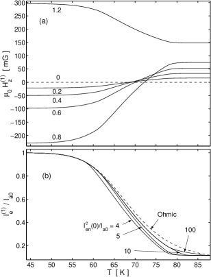
Figure 5: Top: Temperature dependence of the first harmonic $H_{z}^{(1)}$ of the ac self field at positions $x/w=-1.2$, $-0.8$, $-0.6$, $-0.4$, $-0.2$, $0$ on the surface of a long thin strip of width $2w$ with applied ac current $I_{a}=I_{a0}\sin\omega t$. Results within the nonlinear $R_{e}$-model for the same parameters as in Fig. 2 (symmetric case, $\eta=0$) but with $U_{e}(0)=12$, $U_{b}(0)=2$, $I_{en}^{c}(0)/I_{a0}=I_{ex}^{c}(0)/I_{a0}=4$. Assumed was $I_{en}^{c}(T)/I_{en}^{c}(0)=I_{ex}^{c}(T)/I_{ex}^{c}(0)=(1-t)^{2}$ where $t\equiv T/T_{c}$. Bottom: Temperature dependence of the first harmonic $I_{e}^{(1)}$ of the edge current. The parameters are the same as in the top panel but $I_{en}^{c}(0)/I_{a0}=4$ (symmetric case), $5$, $10$, $100$. If $\eta$ differs from zero, the curves remain practically unchanged for $\eta<0.3$. For comparison, the dashed line shows $I_{e}^{(1)}(T)$ for the symmetric Ohmic model with parameters of Fig. 2.

Let us specify the details of this model. With decreasing temperature the currents $I_{en}^{c}$ and $I_{ex}^{c}$ increase, and for definiteness we take $I_{en}^{c}=I_{en}^{c}(0)(1-t)^{2}$, $I_{ex}^{c}=I_{ex}^{c}(0)(1-t)^{2}$ where $t\equiv T/T_{c}$ (such temperature dependence of $I_{en}^{c}+I_{ex}^{c}$ was obtained in Ref. bkv, ). We also imply that near the temperature $T_{sb}$ these critical currents of the edge wires become larger than the amplitude of the applied current $I_{a0}$, and thus the drop of edge-wire resistances occurs at sufficiently high temperatures where conditions (19) are true, and so the inductances and the skin effect are ignored below. As to $R_{en}$, $R_{ex}$ and $R_{b}$, we choose the same expressions for them as in the Ohmic model, but now we use $U_{e}(0)\approx 12$ and $U_{b}(0)\approx 2$ (in units of $T_{c}$), which are essentially less than those used in Sec. III.

To find the first and second harmonics of $H_{z}$, one should solve Eqs. (11)-(13) and find the currents $I_{l}$, $I_{r}$, and $I_{b}$ as functions of $I_{a}$. From these currents, one calculates $H_{z}^{(1)}$, $H_{z}^{(2)}$ using formulas (17)-(18). Within the above simple model, these calculations can be done analytically. For example, in the symmetric case when $\eta=0$ and $I_{en}^{c}=I_{ex}^{c}\equiv I_{e}^{c}/2$, one has formulas (6) for $I_{b}$ and $I_{e}=2I_{l}=2I_{r}$ at $I_{a}\leq I_{1}\equiv I_{e}^{c}\cdot(R_{b}+R_{e})/R_{b}$ where $R_{b}$ and $R_{e}=R_{en}R_{ex}/(R_{en}+R_{ex})$ are independent of $I_{b}$ and $I_{e}$. In the interval $I_{1}\leq I_{a}\leq I_{2}\equiv I_{e}^{c}\cdot(1+w/2r)$ we find $I_{e}=I_{e}^{c}$, $I_{b}=I_{a}-I_{e}^{c}$, while at $I_{2}\leq I_{a}$ equations (11)-(13) yield

$$I_{e} = I_{a}{R_{b}\over R_{b}+0.5R_{0}}=I_{a}\cdot\left(1+{w\over 2r}\right)^{-1},$$

$$I_{b} = I_{a}{0.5R_{0}\over R_{b}+0.5R_{0}}=I_{a}{w\over 2r}\left(1+{w\over 2r}\right)^{-1}.$$ (45)

Using these formulas, we find the following expression for the first harmonic of $I_{e}$:

$$I_{e}^{(1)}\!\!\!\! = \!\!\!\frac{2I_{a0}}{\pi}{R_{b}\over R_{b}+R_{e}}\!\left(\!\phi_{1}\!-\!{\sin 2\phi_{1}\over 2}\!\right)\!+\!\frac{4I_{e}^{c}}{\pi}(\cos\phi_{1}$$ (46)

$$- \!\!\cos\phi_{2})\!+\!\frac{2I_{a0}}{\pi}\!\left(\frac{\pi}{2}\!-\!\phi_{2}\!+\!{\sin 2\phi_{2}\over 2}\!\right)\!\!\left(1+{w\over 2r}\right)^{\!-1}\!\!\!\!\!\!,~{}~{}~{}~{}$$

where $\phi_{1}\equiv\min({\rm arcsin}[I_{1}/I_{a0}],\pi/2)$ and $\phi_{2}\equiv\min({\rm arcsin}[I_{2}/I_{a0}],\pi/2)$. Inserting Eq. (46) into formula (17), we obtain $H_{z}^{(1)}(x)$. The second harmonic of $H_{z}$ in the symmetric case is equal to zero. In Appendix A we present the first and the second harmonics of $H_{z}$ in the asymmetric case when $\eta\neq 0$, $I_{en}^{c}\neq I_{ex}^{c}$. Note that within this nonlinear $R_{e}$ model the characteristic temperature $T_{sb}$ is still defined by the condition $I_{e}^{(1)}=I_{a0}/2$ as in the Ohmic model.

In Fig. 5 we show the first harmonics $H_{z}^{(1)}$ of $H_{z}(t)$ calculated within this nonlinear $R_{e}$ model. The temperature dependence of the first harmonic is qualitatively similar to that of Fig. 2, and with increasing asymmetry of the edge barrier it does not change essentially. On the other hand, the second harmonic $H_{z}^{(2)}$ is highly sensitive to the asymmetry, see Fig. 6. Figure 6 shows both the change of $H_{z}^{(2)}$ with $I_{en}^{c}(0)/I_{ex}^{c}(0)$ at fixed $\eta$ and its change with $\eta$ at fixed $I_{en}^{c}(0)/I_{ex}^{c}(0)$. Interestingly, the temperature dependence of $H_{z}^{(2)}$ is nonmonotonic and looks qualitatively similar to that of Fig. 4. But now the temperature where $H_{z}^{(2)}(T)$ sharply decreases is due to the temperature $T_{1}$ of Appendix A at which some characteristic current of the edge barrier becomes larger than $I_{a0}$. This temperature $T_{1}$ is independent of $\omega$ within our nonlinear $R_{e}$ model. At temperatures $T\leq T_{1}$ during the whole period of the ac field, the currents flowing in the edge wires are less than the appropriate critical currents $I_{en}^{c}$, $I_{ex}^{c}$, the strip is in the Ohmic regime, and $H_{z}^{(1)}(T)$ and $H_{z}^{(2)}(T)$ obtained from the formulas of Appendix A coincide with expressions (38) and (41) if one neglects the inductive terms proportional to $\mu_{0}\omega$ in these expressions. This coincidence permits one to combine this nonlinear model with the Ohmic model of Sec. III and thus to obtain continuous curves in the entire temperature region. Interestingly, when $T$ is larger than the temperature $T_{4}$ of Appendix A, the maximum currents in the edge wires exceed $I_{en}^{c}$ and $I_{ex}^{c}$, and the strip is in the flux-flow regime during some part of the ac period. In Fig. 6 this temperature $T_{4}$ corresponds to the point where $H_{z}^{(2)}(T)$ crosses zero (i.e., $T_{4}\approx 78$ K in Fig. 6b).

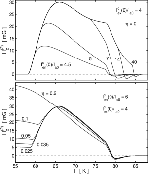
Figure 6: The temperature dependence of the second harmonic of the ac field defined by Eq. (2) at $|x/w|=0.7$ within the nonlinear $R_{e}$ model, Eqs. (18), (60). The parameters are the same as in Fig. 2 but with $U_{e}(0)=12$, $U_{b}(0)=2$, and besides this $I_{ex}^{c}(0)/I_{a0}=4$. The top part shows the second harmonic at fixed $\eta=0$ for different $I_{en}^{c}(0)/I_{a0}=4.5$, $5$, $7$, $14$, $40$, while the bottom part gives this harmonic at fixed $I_{en}^{c}(0)/I_{a0}=6$ but for different asymmetry $\eta=0.025$, $0.035$, $0.05$, $0.1$, $0.2$. Note that $H_{z}^{(2)}(T)$ for $\eta\neq 0$ does not reach zero after its drop in the vicinity of $60$ K.

V Model of nonlinear $R_{b}(I_{b})$

As was mentioned above, in the Ohmic model below a temperature $T_{d}$ defined by the condition $R_{b}(T_{d})\sim\mu_{0}\omega$, the skin effect occurs, which means the perpendicular ac magnetic field $H_{z}$ is expelled from the strip. However, there is another reason for this field to be expelled from the superconductor. Indeed, if the ac current flowing in the bulk is smaller than the critical current $I_{c}=2wdj_{c}$ of the strip, the ac field cannot penetrate completely into the sample. Thus, a finite $I_{c}$ and its increase with decreasing temperature can, in principle, explain the existence of the temperature $T_{d}$ in Fig. 1, below which $H_{z}$ is zero in the strip and at its surface. To describe this, we now consider a nonlinear $R_{b}$ model in which the critical current density $j_{c}$ is not equal to zero, and the resistivity $\rho$ depends on the current density $j$. We shall analyze the following model current–voltage dependence:

$$E=\rho(j)j=\rho_{\rm ff}{jj_{c}\epsilon(j)\over j+j_{c}\epsilon(j)},$$ (47)

where

$$\epsilon(j)=2e^{-U_{0}/T}\sinh\left({j\over j_{c}}{U_{0}\over T}\right),$$ (48)

and $j_{c}$ and the effective depth of flux-pinning well $U_{0}$ are some decreasing functions of $T$. Let us consider the case $U_{0}/T\gg 1$. Then, at $j>j_{c}$ one has $\epsilon(j)\gg j/j_{c}$, and thus $\rho(j)=\rho_{\rm ff}$, while at $j<j_{c}$ the quantity $\epsilon(j)$ is small, $\epsilon(j)\ll j/j_{c}$, and we arrive at $\rho(j)j=\rho_{\rm ff}j_{c}\epsilon(j)\ll\rho_{\rm ff}j$.c2 Thus, equations (47), (48) lead to a sharp jump of resistivity at $j=j_{c}$ that is characteristic for the critical state model. In analytical calculations we shall simplify the model dependence further, putting

$$\rho(j) = \rho_{\rm ff}\ \ \ \ \ {\rm for}\ j>j_{c},$$

$$\rho(j) = 0\ \ \ \ \ \ \ {\rm for}\ j<j_{c}.$$ (49)

As to the flux-flow resistivity $\rho_{\rm ff}$, for definiteness we shall imply the same temperature dependence as in Secs. III and IV, $\rho_{\rm ff}(T)=\rho_{\rm ff}(T_{c})\exp[-U_{b}(0)(1-t)/t]$, where $U_{b}(0)$ is a dimensionless constant and $t\equiv T/T_{c}$. Since in this section we are mainly interested in understanding the effect of nonlinear $R_{b}(I_{b})$ on the first harmonic of the ac field near $T_{d}$, we assume that near $T_{d}$ one has $R_{\rm ff}=\rho_{\rm ff}/2wd\gg\mu_{0}\omega$, $R_{e}$, and the resistances $R_{en}=R_{ex}=2R_{e}$ are independent of $I_{en}=I_{ex}$ (i.e., we treat only the symmetric situation and imply that the skin effect occurs sufficiently below $T_{d}$). The temperature dependence of the critical current $I_{c}=2wdj_{c}$ is assumed to be a monotonically decreasing function. From our analysis it will be clear that this dependence plays the most important role in the vicinity of the temperature $T_{j}$ at which $I_{c}(T)$ reaches $I_{a0}$, and so we may use the following representation of $I_{c}(T)$:

$$I_{c}(T)=I_{a0}\left[T_{c}-T\over T_{c}-T_{j}\right]^{n},$$ (50)

where $n$ is some exponent. Note that in this representation a change of $I_{a0}$ requires a change of $T_{j}$ such that $I_{c}(T)$ remains unchanged.

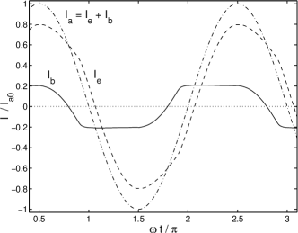
Figure 7: The temporal dependences of the applied current $I_{a}=I_{a0}\sin\omega t$, the bulk current $I_{b}$, and the edge current $I_{e}$ obtained numerically from Eqs. (21)-(25) with the realistic current-voltage dependence (47), (48) at $T=36.5$ K and $U_{0}/T=30$. The other parameters are the same as in Fig. 2 but $U_{b}(0)=6$, $U_{e}(0)=15$, and $I_{a0}=3.57I_{c}$. At this temperature formula (56) gives $I_{2}/I_{c}\approx 3700$. With increasing $I_{a0}$ the width of time intervals where $I_{b}$ changes from $I_{c}$ to $-I_{c}$ or vice versa decreases.

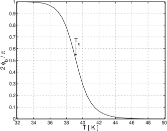
Figure 8: The temperature dependence of the phase shift $\varphi_{b}$ of the bulk current $I_{b}(t)$ as compared to the applied current $I_{a}(t)=I_{a0}\sin\omega t$, Eq. (53). The parameters are the same as in Fig. 2 but $U_{b}(0)=6$, $U_{e}(0)=15$. The temperature $T_{x}\approx 39$ K is defined by Re$\tilde{z}_{e}(T_{x})={\rm Im}\tilde{z}_{e}(T_{x})$, i.e., by $\varphi_{b}\approx\pi/4$.

Let us first show that at $I_{a0}\gg I_{c}=2wdj_{c}$ our nonlinear $R_{b}$ model reduces to the Ohmic model considered in Sec. III. This situation always occurs at sufficiently high temperatures when $I_{c}$ is small. The nonlinearity of $R_{b}(I_{b})$ gives only small corrections to the Ohmic results, and these corrections can be calculated analytically. Indeed, at times $t$ when $I_{b}(t)>I_{c}$, the Ohmic model is applicable, and we have

$$I_{b}=I_{b0}\sin(\omega t+\varphi_{b}),\ \ \ I_{e}=I_{e0}\sin(\omega t+\varphi_{e})$$ (51)

where $I_{b0}$ and $I_{e0}$ are the amplitudes of the currents $I_{b}$ and $I_{e}$,

$$I_{b0} = I_{a0}{|\tilde{z}_{e}|\over|R_{\rm ff}+\tilde{z}_{e}|}\approx I_{a0}{|\tilde{z}_{e}|\over R_{\rm ff}},$$

$$I_{e0} = I_{a0}{R_{\rm ff}\over|R_{\rm ff}+\tilde{z}_{e}|}\approx I_{a0},$$ (52)

the effective impedance of the wires $\tilde{z}_{e}$ is given by Eq. (35), and $\varphi_{b}$, $\varphi_{e}$ define the phase shifts of $I_{b}$ and $I_{e}$ with respect to $I_{a}=I_{a0}\sin\omega t$,

$$\tan\varphi_{b}\approx{{\rm Im}\tilde{z}_{e}\over{\rm Re}\tilde{z}_{e}},\ \ \ \tan\varphi_{e}\approx-{{\rm Im}\tilde{z}_{e}\over R_{\rm ff}}\ll 1.$$ (53)

Formulas (51) - (53) are valid for those times $t$ when $|I_{b}(t)|$ defined by these formulas exceeds $I_{c}$. When the absolute value of $I_{b}(t)$ reaches $I_{c}$, the bulk current $I_{b}$ remains equal to $\pm I_{c}$, while $I_{e}=I_{a}-I_{b}$, see Fig. 7. c3 It is important that $I_{b}$ is uniformly distributed over the width of the strip, $J(x)=\pm I_{c}/2w=\pm j_{c}d$, so long as $|I_{b}|=I_{c}$. This is due to the sharpness of the current-voltage law (V), which prevents the skin effect. A nonuniform distribution of the sheet current $J$ over $x$ occurs only in a relatively narrow time interval (as compared to the period $T=2\pi/\omega$) when $I_{b}$ changes from $I_{c}$ to $-I_{c}$ or vice versa. The relative width of this interval is determined by the small ratio $I_{c}/I_{a0}\ll 1$, and in the first approximation we can neglect this time interval in calculating the first harmonic of $I_{b}(t)$,

$$I_{b}^{(1)}\equiv\frac{2}{T}\int_{0}^{T}I_{b}(t)\sin{\omega t}dt,$$ (54)

which is in-phase with the applied current. Then, we find

$$I_{b}^{(1)}\!\!\!\approx\!\!{2I_{b0}\over\pi}\cos\varphi_{b}\!\cdot\!\!\Big{[}{\pi\over 2}\!-\!\varphi_{2}\!+\!{\sin 2\varphi_{2}\over 2}\!+\!{2I_{2}\over I_{a0}}(1\!-\cos\varphi_{2})\Big{]}\!,~{}$$ (55)

where $\varphi_{2}\equiv\min({\rm arcsin}[I_{2}/I_{a0}],\pi/2)$, $I_{2}$ is the total current at which the amplitude of the bulk current, $I_{b0}$, becomes equal to $I_{c}$,

$$I_{2}\equiv I_{c}{|R_{\rm ff}+\tilde{z}_{e}|\over|\tilde{z}_{e}|}\approx I_{c}{R_{\rm ff}\over|\tilde{z}_{e}|},$$ (56)

and $I_{b0}$, $\varphi_{b}$ are determined by formulas (V), (53). If $I_{a0}\gg I_{2}$, one has $\varphi_{2}\ll 1$, and formula (55) indeed reduces to the result for the Ohmic model, $I_{b}^{(1)}\approx I_{b0}\cos\varphi_{b}$. On the other hand, at $I_{2}>I_{a0}\gg I_{c}$ we have $\varphi_{2}=\pi/2$, and this formula gives

$$I_{b}^{(1)}\approx{4\over\pi}I_{c}\cos\varphi_{b}.$$ (57)

Thus, in this case the temperature dependence of $I_{b}^{(1)}$ is straightforwardly expressed via the temperature dependence of the critical current and of the phase shift $\varphi_{b}$. The dependence $\varphi_{b}(T)$ is shown in Fig. 8. Taking into account that $I_{e}^{(1)}=I_{a0}-I_{b}^{(1)}$ and using formula (17), which is always valid in the absence of the skin effect, we obtain the first harmonic of the magnetic field under condition $I_{a0}\gg I_{c}$, i.e., when the calculated $H_{z}^{(1)}(T)$ does not deviate considerably from the appropriate result of the Ohmic model, see Fig. 9. Here $H_{z}^{(1)}$ is the first harmonic defined by Eq. (1), i.e., its in-phase part.

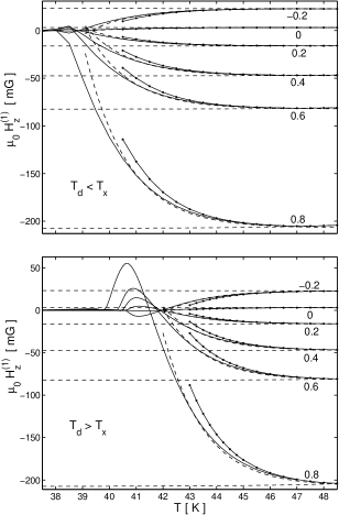
Figure 9: The temperature dependences of the first harmonic $H_{z}^{(1)}$ defined by Eq. (1) within the nonlinear $R_{b}$ model. The parameters are the same as in Fig. 2 but $U_{b}(0)=6$, $U_{e}(0)=15$. The critical current $I_{c}$ is modelled by the power law $I_{c}/I_{a0}=[(T_{c}-T)/(T_{c}-T_{j})]^{30}$ with $T_{j}=37$ K (top) and $T_{j}=40$ K (bottom); $T_{c}=88$ K. This shift of $T_{j}$ from 37 K to 40 K corresponds to the increase of $I_{c}(T)$ by approximately 6.16 times [or equivalently, to the decrease of $I_{a0}$ by 6.16 times at fixed $I_{c}(T)$] and leads to the change of $T_{d}$ from $T_{d}\approx 38.5$ K to $T_{d}\approx 42$ K. The solid lines show the numerical result obtained from Eqs. (21)-(25), (47), (48) with $U_{0}/T=30$, while the solid lines with dots are the analytical result, Eq. (55). The horizontal dashed lines mark $H_{z}^{(1)}$ in the Ohmic model when $I_{c}(T)=0$. The other dashed lines show the analytical approximation obtained from Eqs. (17), (58). The temperature $T_{x}\approx 39$ K, see Fig. 8.

In the nonlinear $R_{b}(I_{b})$ model considered here the temperature $T_{d}$ is of the order of $T_{j}$, and it does not coincide with the temperature at which $R_{b}(T)\sim\mu_{0}\omega$, i.e., with the appropriate temperature for the Ohmic model, $T_{d}^{\rm Ohmic}$ (for the parameters of Fig. 9, $R_{b}\sim\mu_{0}\omega$ at $T_{d}^{\rm Ohmic}\approx 24$ K). The interesting feature of Fig. 9 is that the dependences $H_{z}^{(1)}(T)$ obtained numerically from Eqs. (21) - (25), (47), (48) have different behavior near $T_{d}$ for $T_{j}=37$ K and $T_{j}=40$ K. When $T_{j}=40$ K, one has $\varphi_{b}\approx 0$ everywhere above $T_{d}\approx T_{j}$, see Fig. 8. In other words, the inductance of the edge wires can be disregarded completely. In this case $H_{z}^{(1)}(T)$ has a nonmonotonic behavior near $T_{d}$. When $T_{j}=37$ K, one has $T_{d}\approx 38.5$ K, and this $T_{d}$ lies in the temperature region where the inductance of the edge wires is essential. In this case the curves $H_{z}^{(1)}(T)$ of Fig. 9, in fact, monotonically tend to zero in the vicinity of $T_{d}$. As the boundary of the temperature region where the inductance of the edge wires begins to play a role, one can take the point at which Re$\tilde{z}_{e}={\rm Im}\tilde{z}_{e}$ (i.e., at which $\varphi_{b}\approx\pi/4$). This point is just the temperature $T_{x}$ introduced for the Ohmic model.

In fact, expressions (55), (57) are applicable only for $T>T_{x}$ when $\varphi_{b}\approx 0$, and the dependence $I_{b}^{(1)}(T)$ is determined by $I_{c}(T)$. In the opposite case, at $T<T_{x}$ the phase shift $\varphi_{b}$ rapidly tends to $\pi/2$, and expressions (55), (57) become small. This means that the approximation used in deriving these expressions fails in this region of temperatures. In other words, one cannot neglect the time intervals when $I_{b}$ changes from $I_{c}$ to $-I_{c}$ or vice versa. However, numerical analysis shows that near $T_{d}$, even though $T_{d}<T_{x}$, the dependence $H_{z}^{(1)}(T)$ obtained from Eqs. (21) - (25), (47), (48) can be well approximated by formula (17) if one takes

$$I_{b}^{(1)}(T)\approx I_{c}(T),$$ (58)

see Fig. 9. This statement remains true if instead of Eq. (50) one takes some other form for the temperature dependence of $I_{c}$. It is only important that the function $I_{c}(T)$ be sufficiently sharp near the point $T_{j}$. This finding means that investigation of $H_{z}^{(1)}(T)$ near $T_{d}$ can give information on the temperature dependence of the critical current $I_{c}$ in this temperature region, see Appendix B.

VI Conclusions

To describe the magnetic fields generated by the ac current in the strip, we formally consider the strip as a set of the two edge wires and of wires that form the bulk of the strip. The resistances of all these wires can be nonlinear functions of the currents flowing in them, and the resistances of the edge wires $R_{l}$, $R_{r}$ differ from the resistances of the bulk ones. The resistances of the edge wires characterize the edge barrier, and they are generally different ($R_{l}\neq R_{r}$). To describe the electrodynamics of this strip, we also take into account the inductances of the wires. Equations (21) - (26) provide the description of the magnetic fields and currents in the strip in this general case. We then consider in details three special models which can be useful for understanding the experimental data in various superconductors. The obtained results can be summarized as follows:

Linear (Ohmic) model. In this case the resistances of all the wires are assumed to be independent of the currents flowing in them, and hence the electric fields in the strip are linear functions of these currents. To describe the known experimental data, it is necessary to assume that at $T_{c}$ the resistance of both edge wires $R_{e}$ is larger than the bulk resistance $R_{b}$, but with decreasing temperature $T$, $R_{e}$ decreases sharper than $R_{b}$. The temperatures $T_{sb}$ and $T_{d}$ defined in Fig. 1 can then be found from the conditions: $R_{b}(T_{sb})=R_{e}(T_{sb})$, and $R_{b}(T_{d})\approx\mu_{0}\omega$. The latter condition means that in the Ohmic model at $T_{d}$ the ac magnetic field is expelled from the strip due to the skin effect, and in the vicinity of this $T_{d}$ the inductance of the bulk wires becomes essential. Since $R_{e}(T)$ decreases sharper than $R_{b}(T)$ with decreasing $T$, the inductance of the edge wires begins to play a role at a temperature $T_{x}$ that is higher than $T_{d}$. This $T_{x}$ is defined by Re$\tilde{z}_{e}(T_{x})\approx{\rm Im}\tilde{z}_{e}(T_{x})$ where $\tilde{z}_{e}$ is given by Eq. (35).

We now recite the main features of the Ohmic model. The first harmonic of the ac magnetic field is practically independent of the asymmetry of the edge barrier, $\eta$, which is defined by the asymmetry of the resistances $R_{l}$ and $R_{r}$, Eq. (37), while the second harmonic depends essentially on this asymmetry and exists only at $\eta\neq 0$. The amplitude $H_{z}^{(1)}$ of the first harmonic measured in phase with the applied ac current depends on the frequency $\omega$ only near $T_{d}$, while the magnitude of the second harmonic of the ac field changes with $\omega$ only near $T_{x}$. At $T_{x}$ the magnitude of the second harmonic sharply decreases, and a first harmonic that is out-of-phase with the ac current appears. A characteristic feature of the Ohmic model is also that the ac magnetic field measured in units of $I_{a0}/w$, and hence the temperatures $T_{sb}$, $T_{x}$, $T_{d}$, are independent of the amplitude $I_{a0}$ of the applied current.

Model with nonlinear $R_{e}$. In this model $R_{e}$ (edge) is assumed to be a nonlinear function of the current $I_{e}$ flowing in the edge wires. Namely, we assume the following: If $I_{e}$ exceeds a critical current characterizing the edge barrier, the edge wires do not differ from those in the bulk. But this critical current is implied to increase with decreasing $T$, and when it exceeds $I_{e}$, the resistance $R_{e}$ sharply drops. Thus, in contrast to the Ohmic case, in this model a sharper decrease of $R_{e}(T)$ than of $R_{b}(T)$ is explained by the nonlinear dependence of $R_{e}$ on $I_{e}$. The temperature $T_{sb}$ is now near the temperature at which the above-mentioned critical current reaches $I_{e}$. The temperature dependence of the first harmonic $H_{z}^{(1)}$ is qualitatively similar to that of the Ohmic model, and it does not change essentially with the asymmetry of the edge barrier. On the other hand, the second harmonic of the ac magnetic field is highly sensitive to the asymmetry as in the Ohmic case, but now the temperature where this harmonic sharply drops is due to the temperature $T_{1}$ at which some characteristic current of the edge barrier reaches $I_{a0}$. In this nonlinear model $T_{1}$ is independent of the frequency $\omega$, and it plays the role of the temperature $T_{x}$ marked in Fig. 1.

Model with nonlinear $R_{b}$. In this model $R_{b}$ (bulk) is assumed to be a nonlinear function of the currents flowing in the bulk of the strip, namely: When the critical current for bulk pinning, $I_{c}(T)$, which increases with decreasing $T$, exceeds the bulk current $I_{b}$, the resistance $R_{b}$ sharply drops. Within this model the temperature $T_{d}$ is not due to the skin effect as it occurs for the Ohmic case, but now $T_{d}$ is close to the temperature $T_{j}$ at which the critical current in the strip $I_{c}(T)$ reaches the amplitude $I_{a0}$, $I_{c}(T_{j})=I_{a0}$. Thus, the characteristic feature of this model is that $T_{d}$ depends on the applied amplitude $I_{a0}$ of the applied current rather than on its frequency $\omega$. The temperature dependence of the first harmonic $H_{z}^{(1)}$ near $T_{d}$ is mainly determined by the dependence $I_{c}(T)$; this enables one to extract information on the critical current in this temperature region from the measured $H_{z}^{(1)}(T)$, see Fig. 9 and Appendix B. Interestingly, the shape of $H_{z}^{(1)}(T)$ in the vicinity of $T_{d}$ is different for the cases $T_{d}>T_{x}$ and $T_{d}<T_{x}$ where $T_{x}$ is defined by Re$\tilde{z}_{e}(T_{x})\approx{\rm Im}\tilde{z}_{e}(T_{x})$, i.e., it marks the point where the inductance of the edge wires becomes important.

Different superconductors generally have different dependences $R_{b}(T)$, $R_{e}(T)$, $I_{c}(T)$, and thus are characterized by different values of the parameters that are essential in the formulas of this paper. These parameters also depend on the dimensions of the sample and frequency $\omega$. Therefore, various situations may be expected to occur in experiments; compare, e.g., the data of Refs. 1, and 3, . Possibly, some of them will not be well described by the simple models considered above. However, the above results allow one to understand the data for a specific experiment first qualitatively and then to describe them quantitatively by an improved model.

Appendix A Asymmetric nonlinear $R_{e}$ model

Here we present formulas for the first $H_{z}^{(1)}$ and the second $H_{z}^{(2)}$ harmonics of the ac magnetic field in the framework of the nonlinear model of Sec. IV in the asymmetric case when $I_{en}^{c}/I_{ex}^{c}\geq R_{ex}/R_{en}\geq 1$. Let us introduce the following notations: $q\equiv w/r$,

$$I_{a1}\!\equiv\!I_{ex}^{c}\!\cdot\left(\!1+\!{R_{ex}\over R_{en}}+\!{R_{ex}\over R_{b}}\right)\!,\ \ \ I_{a4}\!\equiv\!I_{en}^{c}\!\cdot(2+q),$$

and

$$I_{a2}\!\equiv\!I_{ex}^{c}\!+I_{en}^{c}\cdot\left(\!1+\!{R_{en}\over R_{b}}\right)\!,\ \ \ I_{a3}\!\equiv\!I_{en}^{c}+I_{ex}^{c}\!\cdot(\!1+q),$$

if $R_{0}/R_{en}>I_{en}^{c}/I_{ex}^{c}$, while if $R_{0}/R_{en}<I_{en}^{c}/I_{ex}^{c}$, we define $I_{a2}$ and $I_{a3}$ as follows:

$$I_{a2}\!\equiv\!I_{ex}^{c}\!\!\cdot\left(\!1\!+\!q\!+\!q{R_{b}\over R_{en}}\!\right)\!,\ \ I_{a3}\!\equiv\!I_{en}^{c}\!\!\cdot\left(\!1\!+\!{R_{en}\over R_{b}}\!+\!q{R_{en}\over R_{b}}\!\right)\!.$$

We also introduce $\phi_{i}\equiv\min({\rm arcsin}[I_{ai}/I_{a0}],\pi/2)$ with $i=1-4$.

The first harmonic $H_{z}^{(1)}(x)$ is determined by $I_{e}^{(1)}$, see Eq. (17). This $I_{e}^{(1)}$ is described by the following long but straightforward expression:

$$I_{e}^{(1)}\!\!\!\! = \!\!\!\frac{2I_{a0}}{\pi}\,{R_{b}\over R_{b}+R_{e}}\!\left(\!\phi_{1}\!-\!{\sin 2\phi_{1}\over 2}\!\right)\!+\frac{4I_{ex}^{c}}{\pi}(\cos\phi_{1}$$ (59)

$$- \!\!\sigma_{1}\cos\phi_{3}\!-\sigma_{2}\cos\phi_{2})\!+\!\frac{4I_{en}^{c}}{\pi}(\sigma_{1}\cos\phi_{2}+\!\sigma_{2}\cos\phi_{3}$$

$$- \cos\phi_{4})\!+\frac{2I_{a0}}{\pi}\,{R_{b}\over R_{b}+R_{en}}\Big{(}\phi_{2}-\phi_{1}-{\sin 2\phi_{2}\over 2}$$

$$+ {\sin 2\phi_{1}\over 2}\Big{)}-\frac{4I_{ex}^{c}}{\pi}\,{R_{b}\over R_{b}+R_{en}}(\cos\phi_{1}-\cos\phi_{2})$$

$$+ \!\frac{2I_{a0}}{\pi(1+q)}\!\left(\phi_{4}\!-\!\phi_{3}\!+\!{\sin 2\phi_{3}\over 2}\!-{\sin 2\phi_{4}\over 2}\right)\!\!$$

$$- \frac{4I_{en}^{c}}{\pi(1+q)}(\cos\phi_{3}-\!\cos\phi_{4})+\frac{4I_{a0}}{\pi(2+q)}\Big{(}{\pi\over 2}-\!\phi_{4}\!$$

$$+ \!{\sin 2\phi_{4}\over 2}\!\Big{)}\!+\sigma_{2}\frac{2I_{a0}}{\pi}\,{qR_{b}+R_{en}\over q(R_{b}+R_{en})+R_{en}}\Big{(}\phi_{3}\!-\!\phi_{2}$$

$$+ \!{\sin 2\phi_{2}\over 2}-{\sin 2\phi_{3}\over 2}\Big{)}\,,$$

where $\sigma_{1}=1$ if $R_{0}/R_{en}>I_{en}^{c}/I_{ex}^{c}$ and $\sigma_{1}=0$ otherwise, while $\sigma_{2}=1-\sigma_{1}$. In the symmetric case when $I_{en}^{c}/I_{ex}^{c}=R_{ex}/R_{en}=1$, one has $R_{en}=R_{ex}=2R_{e}$, $I_{en}^{c}=I_{ex}^{c}=I_{e}^{c}/2$, $\sigma_{2}=0$, $I_{a1}=I_{a2}=I_{1}$, $I_{a3}=I_{a4}=I_{2}$ where the currents $I_{1}$, $I_{2}$ are defined in Sec. IV. In this case formula (59) reduces to Eq. (46).

According to formula (18), the second harmonic is determined by $\Delta I_{e}^{(2)}$. This $\Delta I_{e}^{(2)}$ is given by:

$$\Delta I_{e}^{(2)}\!\!\!\! = \!\!\!I_{a0}{(R_{ex}-R_{en})\over(R_{ex}+R_{en})}\,{R_{b}\over R_{b}+R_{e}}\!\left(\!{1\over 3}-\!{\cos\phi_{1}\over 2}+{\cos 3\phi_{1}\over 6}\!\right)\!$$ (60)

$$+ I_{a0}{R_{b}\over R_{b}+R_{en}}\Big{(}{\cos\phi_{1}\over 2}-{\cos 3\phi_{1}\over 6}-{\cos\phi_{2}\over 2}$$

$$+ {\cos 3\phi_{2}\over 6}\Big{)}+I_{ex}^{c}{2R_{b}+R_{en}\over R_{b}+R_{en}}\Big{(}{\sin 2\phi_{2}\over 2}-{\sin 2\phi_{1}\over 2}\Big{)}$$

$$+ \!I_{en}^{c}\,{(2+q)\over 2(1+q)}(\sin 2\phi_{3}-\!\sin 2\phi_{4})+\!{I_{a0}\over(1+q)}\Big{(}{\cos\phi_{4}\over 2}$$

$$- \!\!\!{\cos 3\phi_{4}\over 6}-\!{\cos\phi_{3}\over 2}+\!{\cos 3\phi_{3}\over 6}\!\Big{)}\!+\!\sigma_{1}\!{(\!I_{en}^{c}\!\!-\!I_{ex}^{c})\over 2}(\sin 2\phi_{2}$$

$$- \!\sin 2\phi_{3})+\sigma_{2}I_{a0}{qR_{b}-R_{en}\over q(R_{b}+R_{en})+R_{en}}\Big{(}{\cos\phi_{2}\over 2}$$

$$- {\cos 3\phi_{2}\over 6}-{\cos\phi_{3}\over 2}+{\cos 3\phi_{3}\over 6}\Big{)}.$$

In the symmetric case the quantity $\Delta I_{e}^{(2)}$ vanishes, as it should be.

We now present formulas for the resistance $R$ of the strip in this model. Such formulas may be useful to compare data obtained from the ac experiments and from the conventional transport measurements. Let us define four temperatures $T_{i}$ as temperatures at which $\tilde{I}_{ai}(T_{i})=1$, where $\tilde{I}_{ai}(T)\equiv I_{ai}(T)/I_{a0}$, $i=1-4$, and $I_{a0}$ is the applied transport current. Then, one has

$$R\! = \!{R_{b}R_{e}\over R_{b}+R_{e}}\ \ \ \ \ \ \ \ \ \ \ \ \ \ \ \ \ {\rm for}\ T\leq T_{1},$$

$$R\! = \!{R_{b}R_{en}\over R_{b}+R_{en}}(1-\tilde{I}_{ex}^{c})\ \ \ \ {\rm for}\ T_{1}\leq T\leq T_{2},$$

$$R\! = \!\sigma_{1}R_{b}(1\!-\!\tilde{I}_{ex}^{c}\!-\!\tilde{I}_{en}^{c})+{\sigma_{2}qR_{b}R_{en}\over q(R_{b}\!+\!R_{en})\!+\!R_{en}}$$ (61)

$$\ \ \ \ \ \ \ \ \ \ \ \ \ \ \ \ \ \ \ \ \ \ \ \ \ \ \ \ \ {\rm for}\ T_{2}\leq T\leq T_{3},$$

$$R\! = \!R_{b}{q\over(1+q)}(1-\tilde{I}_{en}^{c})\ \ \ \ \ {\rm for}\ T_{3}\leq T\leq T_{4},$$

$$R\! = \!R_{b}{q\over(2+q)}\ \ \ \ \ \ \ \ \ \ \ \ \ \ \ \ \ {\rm for}\ T_{4}\leq T,$$

where $\tilde{I}_{en}^{c}\equiv I_{en}^{c}/I_{a0}$ and $\tilde{I}_{ex}^{c}\equiv I_{ex}^{c}/I_{a0}$. Note that $R$ is independent of the applied current $I_{a0}$ at $T<T_{1}$ and at $T>T_{4}$. Besides this, if $R_{0}/R_{en}=I_{en}^{c}/I_{ex}^{c}$ at some temperature $T_{*}$, and if the interval $T_{2}-T_{3}$ lies above $T_{*}$, a current-independent resistance occurs in this interval as well.

Appendix B Extraction of $I_{c}(T)$ from experimental data

If the nonlinear $R_{b}$ model is applicable to describe some experimental data on $H_{z}^{(1)}(T)$ near the temperature $T_{d}$, the critical current $I_{c}(T_{d})$ can be approximately estimated from the relations $I_{c}(T_{j})=I_{a0}$ and $T_{d}\approx T_{j}$. Changing $I_{a0}$, one finds $I_{c}(T)$ in some temperature interval which is determined by the range of $I_{a0}$. On the other hand, the temperature dependence $I_{c}(T)$ can be also estimated from the shape of the curves $H_{z}^{(1)}(T)$ measured at fixed $I_{a0}$. Using the approximation (58) and formula (17), we obtain

$$I_{c}(T)={2wH_{z}^{(1)}(T)-I_{a0}\cdot g\over f-g},$$ (62)

where $H_{z}^{(1)}(T)$ is the first harmonic measured at an inner point $x$ (i.e., at $|x|<w$), $g=(xw/\pi)/(w^{2}-x^{2})$, $f=2wH_{z}^{(1)}(T_{c})/I_{a0}$, and $H_{z}^{(1)}(T_{c})$ is the first harmonic $H_{z}^{(1)}$ measured at the same point $x$ at a temperature near $T_{c}$. Here, to express $f$ in terms of $H_{z}^{(1)}(T_{c})$, we have used formula (17) again and have taken into account that at $T=T_{c}$ the edge barrier is absent, and $I_{b}^{(1)}=I_{a0}$. When the sample is an “ideal” strip (i.e., uniform with constant thickness, width, and homogeneous critical current density), one has $f=(1/2\pi)\ln(|w-x|/|w+x|)$. Note that these two ways of estimating $I_{c}$ more reliably give the temperature dependence of $I_{c}$ rather than the absolute value of the critical current. Indeed, at $T=T_{d}$ when one has $H_{z}^{(1)}(T)=0$, the first method gives $I_{c}=I_{a0}$, while the second method leads to $I_{c}=I_{a0}\cdot g/(g-f)\approx I_{a0}/2$. This discrepancy is caused by the inaccuracy of the relation $T_{d}\approx T_{j}$ and of the approximation (58).

References

- (1) D. T. Fuchs, E.Zeldov, M. Rappaport, T. Tamegai, S. Ooi, and H. Shtrikman, Nature 391, 373 (1998).
- (2) D. T. Fuchs, E. Zeldov, T. Tamegai, S. Ooi, M. Rappaport, and H. Shtrikman, Phys. Rev. Lett. 80, 4971 (1998).
- (3) Y. Paltiel, D. T. Fuchs, E. Zeldov, Y. N. Myasoedov, H. Shtrikman, M. L. Rappaport, and E. Y. Andrei, Phys. Rev. B 58, R14763 (1998).
- (4) L. Burlachkov, A. E. Koshelev, and V. M. Vinokur, Phys. Rev. B 54, 6750 (1996).
- (5) J. R. Clem, in Proceedings of Low Temperature Physics-LT 13, edited by K. D. Timmerhaus, W. J. O’Sullivan, and E. F. Hammel (Plenum, New York, 1974), Vol. 3, p. 102.
- (6) E. Zeldov, A. I. Larkin, V. B. Geshkenbein, M. Konczykowski, D. Majer, B. Khaykovich, V. M. Vinokur, H. Shtrikman, Phys. Rev. Lett. 73, 1428 (1994).
- (7) L.D. Landau and E.M. Lifshits, Electrodynamics of Continuous Media, Course in Theoretical Physics Vol. 8 (Pergamon, London, 1959).
- (8) E. H. Brandt, Phys. Rev. B64, 024505 (2001).
- (9) E. H. Brandt, Phys. Rev. B73, 092511 (2006).
- (10) However, we shall still assume that there is no skin effect across the thickness of the strip . This is not a restrictive assumption since the ac magnetic field is completely expelled from the sample before such effect occurs at lower temperatures.
- (11) D. T. Fuchs, R. A. Doyle, E. Zeldov, S. F. W. R. Rycroft, T. Tamegai, S. Ooi, M. L. Rappaport, and Y. Myasoedov, Phys. Rev. Lett. 81, 3944 (1998).
- (12) T. T. M. Palstra, B. Batlogg, L. F. Schneemeyer, J. V. Waszczak, Phys. Rev. Lett. 61, 1662 (1988).
- (13) T. T. M. Palstra, B. Batlogg, R. B. van Dover, L. F. Schneemeyer, J. V. Waszczak, Phys. Rev. B41, 6621 (1990).
- (14) R. Busch, G. Ries, H. Werthner, G. Kreiselmeyer, G. Saemann-Ischenko, Phys. Rev. Lett. 69, 522 (1992).
- (15) Beside this, if one reaches by changing , the shapes of the curves Re differ noticeably from those of Fig. 1.
- (16) In the limit expressions (47), (48) reproduce the well-known thermally assisted flux flow (TAFF) regime.
- (17) Note that Fig. 7 has been plotted for the realistic current-voltage law, Eqs. (47) and (48), rather than for the idealized model (V).