Flat spin wave dispersion in a triangular antiferromagnet

Abstract

The excitation spectrum of a $S=1/2$ 2D triangular quantum antiferromagnet is studied using $1/S$ expansion. Due to the non-collinearity of the classical ground state significant and non-trivial corrections to the spin wave spectrum appear already in the first order in $1/S$ in contrast to the square lattice antiferromagnet. The resulting magnon dispersion is almost flat in a substantial portion of the Brillouin zone. Our results are in quantitative agreement with recent series expansion studies by Zheng, Fjærestad, Singh, McKenzie, and Coldea [Phys. Rev. Lett. 96, 057201 (2006) and cond-mat/0608008].

Triangular antiferromagnets occupy a special niche in the studies of quantum magnetism. Ising antiferromagnet on triangular lattice has a finite zero-temperature entropy, which reflects an extensive degeneracy of the ground state manifold wannier . Classical Heisenberg model on a triangular lattice represents the textbook example of the full $SU(2)$ symmetry breaking and noncollinear spiral spin ordering in the ground state - the $120^{\circ}$ spin structure. For a quantum $S=1/2$ antiferromagnet on a triangular lattice, Anderson proposed back in 1973 the disordered resonating valence bond (RVB) ground state rvb . This suggestion stimulated extensive research for over 25 years. An RVB ground state on a triangular lattice has been found recently qdm-rvb , albeit for a quantum dimer model. It was also established, by large-N and gauge theory approaches, that a disordered ground state of a triangular antiferromagnet must possess unconfined massive spinon excitations read-sachdev .

On the experimental side, several novel materials with triangular structure have attracted substantial interest over the last few years. $Na_{x}CoO_{2}$, in which $Co$ atoms form a layered hexagonal structure nacoo , was suggested to be in close proximity to a spin liquid lee . Another potential candidate for a spin liquid is $\kappa-(ET)_{2}Cu_{2}(CN)_{3}$ at small pressures kanoda . Finally, there is an intensive theoretical debate veillette1 ; veillette2 ; dalidovich ; alicea on the structure of the ground state of a spatially anisotropic triangular $S=1/2$ antiferromagnet $Cs_{2}CuCl_{4}$ coldea2001 .

The ideas about the disordered ground state of unconfined spinons, however, could not be immediately applied to the most studied Heisenberg model of quantum $S=1/2$ spins on a triangular lattice, as both perturbative $1/S$ and numerical calculations point that the classical, $120^{\circ}$ spin structure survives quantum fluctuations. Quantum fluctuations do reduce the average value of a sublattice magnetization to $50\%$ of its classical value css . This renormalization is generally comparable to that for a $S=1/2$ antiferromagnet on the square lattice igarashi . For the latter, calculations to order $1/S^{2}$ for the spectrum do show that the overall scale of the spin-wave dispersion is renormalized by quantum fluctuations, but the dispersion retains almost the same functional form as in the quasiclassical limit, and obviously is better described by magnons rather than by deconfined spinons.

For a triangular antiferromagnet, Chubukov et al css computed $1/S$ corrections to the two spin-wave velocities, and found that these corrections are quite small, even for $S=1/2$. No $1/S$ calculations of the full spin-wave dispersion have been reported in the literature but, based on the results for the velocities, it was widely believed that the functional form of the dispersion for $S=1/2$ antiferromagnet should also be close to that in the quasiclassical, large $S$ limit, i.e., that the spin-wave description can be extended to $S=1/2$. Recent series expansion study rajiv_1 , however, uncovered remarkable changes in the functional form of the dispersion in the isotropic quantum $S=1/2$ antiferromagnet on triangular lattice compared to $S=\infty$ limit. In particular, the dispersion for the $S=1/2$ case possesses local minima (“rotons”) at the mid-points of faces of the hexagonal Brillouin zone (BZ). The classical dispersion does not have such local minima.

The authors of Ref. rajiv_1 conjectured that the qualitative changes between the actual dispersion for $S=1/2$ and the classical dispersion may imply that at energies comparable to the exchange integral $J$, the system is better described in terms of pairs of deconfined spinons rather than magnons (the latter in such description are bound states of spinons). In other words, they argued that the spinon description, valid for the disordered state, may adequately describe high-energy excitations of the ordered state.

In this communication, we propose another explanation for the series expansion results, alternative to the one proposed in Ref. rajiv_1 . We argue that regular 1/S corrections, extended to $S=1/2$, strongly modify the form of the magnon dispersion in a triangular antiferromagnet, and the renormalized dispersion has “roton” minima at the faces of the BZ, in agreement with rajiv_1 . But we also found a more drastic effect – the renormalized dispersion turns out to be almost flat in a wide range of momenta. The flat renormalized dispersion has not been reported in rajiv_1 where the numerical data have been presented only along special high-symmetry directions in the BZ. The subsequent, more detailed series expansion studies rajiv_2 , carried out in parallel with our research, did find the regions of flat dispersion. The analytical and series expansion results are in good qualitative and quantitative agreement, which indicates that the flat regions are likely present in the actual dispersion, and that a first order in $1/S$ provides fairly accurate description of a triangular antiferromagnet even at high energies, comparable to the exchange $J$.

The point of departure for the $1/S$ calculation is the Heisenberg antiferromagnet on a triangular lattice

$${\cal H}=J\sum_{<i,j>}{\bf S}_{i}{\bf S}_{j}.$$ (1)

Using Holstein-Primakoff transformation to bosons, assuming the $120^{\circ}$ spin structure in the ground state, and diagonalizing the quadratic form in bosons one can re-write Eq. (1) as css

$${\cal H}=3JS\left[\sum_{k}E_{k}c^{\dagger}_{k}c_{k}+\frac{1}{\sqrt{S}}{\cal H}_{3}+\frac{1}{S}{\cal H}_{4}+...\right],$$ (2)

where dots stand for higher order terms in $1/S$, and

$$E_{k}=\sqrt{A^{2}_{k}-B^{2}_{k}}=\sqrt{(1-\nu_{k})(1+2\nu_{k})},$$ (3)

where

$$A_{k} = 1+\frac{\nu_{k}}{2},~{}B_{k}=-\frac{3}{2}\nu_{k},$$

$$\nu_{k} = \frac{1}{3}\left(\cos{k_{x}}+2\cos{\frac{k_{x}}{2}}\cos{\frac{\sqrt{3}k_{y}}{2}}\right).$$ (4)

The BZ is presented in Fig. 1. The magnon energy $E_{k}$ vanishes at the center of the zone, $k=0$, where $\nu_{k}=1$, and at the corners of the BZ (e.g. at points Q and C), where $\nu_{k}=-1/2$.

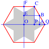
Figure 1: (Color online) BZ of a triangular antiferromagnet. Thin lines indicate the directions along which the “cuts” of dispersion are taken. Coordinates of the points are: P$(2\pi/3,0)$, A$(\pi,0)$, Q$(4\pi/3,0)$, B$(\pi,\pi/\sqrt{3})$, C$(2\pi/3,2\pi/\sqrt{3})$, F$(0,2\pi/\sqrt{3})$, and E$(0,\pi/\sqrt{3})$. ${\text{Im}}\Sigma^{(S)}_{k}\neq 0$ inside the shaded star-shaped area.

In a square-lattice antiferromagnet, ${\cal H}_{3}$ term is absent, and $1/S$ corrections to the dispersion come from the decoupling of the four-boson term. These corrections do not affect the functional form of the dispersion igarashi . The corrections to the dispersion then appear at $1/S^{2}$ order, from ${\cal H}_{6}$ term in the magnon Hamiltonian and from the second-order perturbation in ${\cal H}_{4}$, both are very small numerically. In triangular antiferromagnets, ${\cal H}_{3}$ term is present due to the non-collinearity of the classical spin configuration ($120^{\circ}$ structure) and, taken at the second order, gives rise to non-trivial corrections to the dispersion already at the order $1/S$. The expressions for ${\cal H}_{3}$ and ${\cal H}_{4}$ have been obtained in css and we refer to that work for the derivation. Decoupling the four-magnon term in a standard way and adding the result to the quadratic form we obtain, to order $1/S$,

$${\cal H}=3JS\left[\sum_{k}{\bar{E}}_{k}c^{\dagger}_{k}c_{k}+\frac{1}{\sqrt{S}}{\cal H}_{3}\right],$$ (5)

where ${\bar{E}}_{k}$ represents dispersion renormalized by quartic terms (coming from ${\cal H}_{4}$ css )

$${\bar{E}}_{k}^{2}=E_{k}^{2}(1+c_{1}/S)+(1-\nu_{k})c_{2}/S,$$ (6)

where $c_{1}=1-I_{0}-I_{1}/4+5I_{2}/4,~{}c_{2}=3(I_{2}-I_{1})/4$ and $I_{n}=\frac{1}{N}\sum_{k}\nu_{k}^{n}/E_{k}$. The cubic part reads

$${\cal H}_{3}=i\left(\frac{3}{32N}\right)^{1/2}\sum_{1,2}\Big{(}c^{\dagger}_{1}c^{\dagger}_{2}c_{k}\Phi_{1}(1,2,k)\delta_{1+2-k}$$

$$+\frac{1}{3}c^{\dagger}_{1}c^{\dagger}_{2}c^{\dagger}_{k}\Phi_{2}(1,2,k)\delta_{1+2+k}+{\text{h.c.}}\Big{)}.$$ (7)

Here $1=k_{1}$, $2=k_{2}$, and summation is over the BZ. The vertices $\Phi_{1,2}(1,2,k)={\tilde{\Phi}}_{1,2}(1,2,k)/\sqrt{E_{1}E_{2}E_{k}}$, where

$${\tilde{\Phi}}_{1,2}(1,2,3)={\bar{\nu}}_{1}f^{(1)}_{-}\left(f^{(2)}_{+}f^{(3)}_{+}\pm f^{(2)}_{-}f^{(3)}_{-}\right)+{\bar{\nu}}_{2}f^{(2)}_{-}\times$$

$$\left(f^{(1)}_{+}f^{(3)}_{+}\pm f^{(1)}_{-}f^{(3)}_{-}\right)+{\bar{\nu}}_{3}f^{(3)}_{-}\left(f^{(1)}_{+}f^{(2)}_{+}-f^{(1)}_{-}f^{(2)}_{-}\right)$$ (8)

are expressed in terms of $f^{(i)}_{\pm}=\sqrt{A_{k_{i}}\pm B_{k_{i}}}$ and

$${\bar{\nu}}_{k}=\frac{2}{3}\sin\frac{k_{x}}{2}\left(\cos\frac{k_{x}}{2}-\cos\frac{\sqrt{3}k_{y}}{2}\right).$$ (9)

The ${\cal H}_{3}$ term gives rise to a $k$-dependent magnon self-energy to order $1/S$

$$\Sigma_{k}^{(S)} = -\frac{3}{16SN}\Big{(}\sum_{1+2=k}\frac{|\Phi_{1}(1,2,k)|^{2}}{E_{1}+E_{2}-E_{k}+i0}$$ (10)

$$+\sum_{1+2=-k}\frac{|\Phi_{2}(1,2,k)|^{2}}{E_{1}+E_{2}+E_{k}+i0}\Big{)}.$$

Note that at this order $\Phi_{1,2}$ and $E_{k}$ are expressed via bare ($S=\infty$) quantities. Collecting the corrections from three-magnon and four-magnon processes and restoring the pre-factor $3JS$ (see Eq. 5), we obtain for the full renormalized dispersion

$$E_{\text{ren}}(k)=3JS\sqrt{{\bar{E}}_{k}^{2}+2E_{k}\Sigma_{k}^{(S)}}.$$ (11)

Expanding (11) to first order in $1/S$ we finally obtain

$$E_{\text{ren}}(k)=3JS\left[E_{k}(1+\frac{c_{1}}{2S})+\frac{(1-\nu_{k})c_{2}}{2SE_{k}}+\Sigma_{k}^{(S)}\right].$$ (12)

It was shown in css that the renormalized dispersion preserves zeros at $k=0$ and at the corners of the BZ, i.e., locations of Goldstone modes are not affected by $1/S$ corrections. Below we compute the full spin-wave dispersion (12) and apply the results to $S=1/2$.

We used the Mathematica© software to calculate the self-energy $\Sigma_{k}$, (10). Two-dimensional momentum integrals were regularized by replacing energy denominators with $E+i\delta$, where $\delta=10^{-4}$, and taking the real part of the resulting expression. The imaginary part was calculated using the “bell approximation” for the delta function: $\delta(x)=\sqrt{t/\pi}e^{-tx^{2}}$. We found that $t=10^{3}$ gives stable and consistent results.

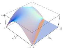
(a)

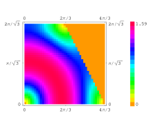
(b)

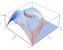
(c)

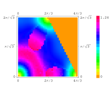
(d)

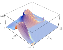
(e)

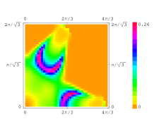
(f)

Figure 2: (Color online) Classical and renormalized spin wave dispersions. Left panels – three-dimensional plots, right panels – color density plots. The dispersions are shown in the OQCF quadrant of the BZ and are set to zero outside this region to ease the viewing. The classical dispersion, figures (a,b), is $1.5E_{k}$. The real part of renormalized dispersion $E_{\text{ren}}(k)$ (Eq. 12) is shown in figures (c) and (d). The flat dispersion is in the blue (dark) region in (d). The imaginary part of the renormalized dispersion is shown in figures (e, f). Observe that it is numerically small throughout the BZ, and is zero outside the “star” region, see also Fig 1.

Our results are shown as three-dimensional plots in Fig 2. For comparison we also plotted the classical dispersion $3JSE_{k}=1.5JE_{k}$. For clarity, we only plot the dispersion over a quarter of the BZ, and set it to zero outside this quarter. Observe that the renormalized dispersion vanishes at $k=0$ and at the corners of the BZ hexagon. Spin wave velocity at $k=0$ decreases in comparison to the classical result, while the one at the corners of the BZ increases (see Fig 4(a) below) css .

We clearly see from Fig 2 that the actual dispersion is rather different from $1.5E_{k}$. The key difference is that the renormalized dispersion $E_{\text{ren}}(k)$ has a plateau at around $0.8J$ over a wide range of momenta. This is most clearly seen in Fig  2(c) and 2(d). The dispersion also possesses a roton-like minimum near the faces of the BZ, as is best seen along the cut FC, Fig 3(a).

In Fig 2(e) and 2(f) we show the imaginary part of $E_{\text{ren}}(k)$ from three-magnon processes. In distinction to a square-lattice antiferromagnet, the imaginary part of the dispersion in our case appears already at the order $1/S$. As follows from (10), it is present when one-particle excitation (magnon) with momentum $\vec{k}$ can decay into the two-particle continuum, i.e., when $E_{\vec{q}}+E_{\vec{k}-\vec{q}}=E_{\vec{k}}$ for some $\vec{q}\in$ BZ. This condition defines star-shaped region, shown in light gray shading in Fig 1 (see also Fig 2(f)): inside it ${\text{Im}}\Sigma^{(S)}_{k}$ is nonzero. While ${\text{Im}}\Sigma^{(S)}_{k}\neq 0$ (and, hence, ${\text{Im}}E_{\text{ren}}(k)\neq 0$) in most of the BZ, we found that ${\text{Im}}E_{\text{ren}}(k)$ does not exceed $0.26J$, and is much smaller than ${\text{Re}}E_{\text{ren}}(k)$. Nonetheless, a finite imaginary part is important as it responsible for dampening excitations at wavevectors where variations of ${\text{Re}}E_{\text{ren}}(k)$ in Fig 2(c) and 2(d) are maximal.

Observe that the maxima of ${\text{Im}}E_{\text{ren}}(k)$ in Fig 2(e) occur exactly where the variation of ${\text{Re}}E_{\text{ren}}(k)$ is the strongest, see also Figs 3-5 below. In other words, the sharp features in the $1/S$ dispersion are not artefacts of numerical calculations, but are real features of the excitation spectrum at this order. Observe also that ${\text{Im}}E_{\text{ren}}(k)$ vanishes at momenta where ${\text{Re}}E_{\text{ren}}(k)$ stays almost constant. This implies that nearly immobile magnons have infinite lifetime, i.e., are true excited states of the system.

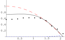
(a)

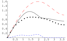
(b)

Figure 3: (Color online) Classical and renormalized dispersions (ordinate) along (a) FC and (b) OF directions (abscissa). Red dashed line - classical dispersion. Black solid line – the real part of the renormalized dispersion $E_{\text{ren}}(k)$, Eq. (12). Blue dotted line - the imaginary part of $E_{\text{ren}}(k)$. The black dots are series expansion data from rajiv_2 . No fitting parameter is involved in the comparison with the data.

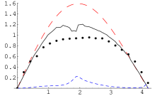
(a)

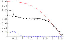
(b)

Figure 4: (Color online) Same as in Fig. 3 but along (a) OQ and (b) PC directions.

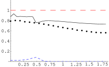
(a)

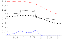
(b)

Figure 5: (Color online) Same as in Fig. 3 but along (a) AB and (b) EB directions.

To better display the new features and for comparison with series expansion studies, we show in Figs 3-5 the dispersion $E_{\text{ren}}(k)$ along six different cuts through the BZ (black lines). The directions of particular cuts are shown in Fig 1. In each of the plots, we also show the classical dispersion (dashed red lines). The flat regions are clearly seen in the cuts along FC, OF, PC, and EB directions, and the roton minimum is seen in the cut along FC direction. Note that in accordance with Fig 1, the local minimum near point F (Fig 3(a)) corresponds to a truly stable excitation, ${\text{Im}}E_{\text{ren}}(k)=0$ there. The maximum of the renormalized dispersion is at $1.2J$ which is substantially smaller than $1.6J$ for the classical dispersion.

We now compare in some detail our results to series expansion studies of Zheng et al rajiv_1 ; rajiv_2 . First, series expansion studies have found that the dispersion has a bandwidth of about $J$ (see series data in Fig 4(b)), which is substantially smaller than $1.6J$ for a classical dispersion. This is in agreement with our results (see Figs. 3-5). Note that this difference is much larger than one might expect by comparing the spin-wave velocities which are renormalized only by about 10% css . Second, series expansion studies found “roton” minima near points F and B in the BZ, Fig 1. Our cuts along FC and OF also show a minumum near point F (see Fig 3). Third, recent series expansion studies rajiv_2 found the regions of flat dispersion at $0.8J$ along FC, PC, and EB directions. Our results for $E_{\text{ren}}(k)$ also show the regions of flat dispersion at around $0.8-0.9J$. The flat regions are clearly seen on the density plot in Fig 2(d), as well as in Figs 3(a),  4(b), and in Fig 5(b) (near points E and B).

The near-flat regions of the magnon dispersion have a large density of states and can be probed by Raman scattering. The two-magnon Raman intensity in a square-lattice antiferromagnet is peaked slightly below twice the frequency at which the magnon density of states diverges. In our case, the density of states is peaked at around $0.8J$, and we expect that the two-magnon Raman intensity will be peaked somewhat below $1.6J$.

To conclude, in this paper we used $1/S$ expansion, extended it to $S=1/2$, and obtained the renormalized magnon dispersion for a Heisenberg antiferromagnet on triangular lattice. We found that the renormalized dispersion is qualitatively different from the classical one – it is almost flat over a wide range of momenta in the BZ, and has roton-like minuma near the mid-points of faces of the BZ. These results are in full agreement with recent series expansion studies.

We are thankful to R.R.P. Singh for valuable discussion and to R.R.P. Singh and W. Zheng for sending us series expansion results prior to publication. OAS acknowledges the donors of the American Chemical Society Petroleum Research Fund for support (PRF43219-AC10). AVC and AGA are supported by NSF via grants No. DMR-0240238 and DMR-0348358, respectively. The authors thank the Theory Institute at Brookhaven National Laboratory where this work has initiated.

Note added: after submission of our manuscript we learned of a closely related study of magnon decays in triangular antiferromagnets sasha-misha .

References

- (1) G.H. Wannier, Phys. Rev. 79, 357-364 (1950).
- (2) P.W. Anderson, Mater. Res. Bull. 8, 153 (1973); P. Fazekas and P.W. Anderson, Philos. Mag. 30, 423 (1974).
- (3) R. Moessner and S.L. Sondhi, Phys. Rev. Lett. 86, 1881 (2001).
- (4) N. Read and S. Sachdev, Phys. Rev. Lett. 66, 1773 (1991); A.V. Chubukov, S. Sachdev, and T. Senthil, Nucl. Phys. B 426, 601 (1994).
- (5) K. Takada, H. Sakurai, E. Takayama-Muromachi, F. Izumi, R.A. Dilanian, and T. Sasaki, Nature 422, 53 (2003).
- (6) S. Zhou, M. Gao, H. Ding, P.A. Lee, and Z. Wang, Phys. Rev. Lett. 94, 206401 (2005).
- (7) Y. Shimizu, K. Miyagawa, K. Kanoda, M. Maesato, and G. Saito, Phys. Rev. Lett. 91, 107001 (2003).
- (8) R. Coldea, D.A. Tennant, A.M. Tsvelik, and Z. Tylczynski, Phys. Rev. Lett. 86, 1335 (2001).
- (9) M.Y. Veillette, J.T. Chalker, and R. Coldea, Phys. Rev. B71, 214426 (2005).
- (10) M.Y. Veillette, A.J.A. James, and F.H.L. Essler, Phys. Rev. B72, 134429(2005).
- (11) D. Dalidovich, R. Sknepnek, A.J. Berlinsky, J. Zhang, and C. Kallin, Phys. Rev. B73, 184403 (2006).
- (12) J. Alicea, O.I. Motrunich, and M.P.A. Fisher, Phys. Rev. Lett. 95, 247203 (2005).
- (13) W. Zheng, J.O. Fjærestad, R.P.P. Singh, R.H. McKenzie, and R. Coldea, Phys. Rev. Lett. 96, 057201 (2006).
- (14) W. Zheng, J.O. Fjærestad, R.P.P. Singh, R.H. McKenzie, and R. Coldea, cond-mat/0608008.
- (15) A.V. Chubukov, S. Sachdev, and T. Senthil, J.Phys.: Condensed Matter 6, 8891 (1994).
- (16) J. Igarashi, Phys. Rev. B46, 10763 (1992); J. Igarashi and T. Nagao, Phys. Rev. B72, 014403 (2005).
- (17) A.L. Chernyshev and M.E. Zhitomirsky, Phys. Rev. Lett. 97, 207202 (2006).