Local Spectral Weight of a Luttinger Liquid: Effects from Edges and Impurities

Abstract

We calculate the finite-temperature local spectral weight (LSW) of a Luttinger liquid with an ”open” (hard wall) boundary. Close to the boundary the LSW exhibits characteristic oscillations indicative of spin-charge separation. The line shape of the LSW is also found to have a Fano-like asymmetry, a feature originating from the interplay between electron-electron interaction and scattering off the boundary. Our results can be used to predict how edges and impurities influence scanning tunneling microscopy (STM) of one-dimensional electron systems at low temperatures and voltage bias. Applications to STM on single-walled carbon nanotubes are discussed.

I Introduction

Metallic electrons confined to one dimension exhibit a plethora of intriguing effects, driven by interactions and the coupling to impurities and defects Giamarchi . At low energies a clean system is described by the concept of a spinful Luttinger liquid (LL) Voit , with properties very different from those of a Fermi liquid: the quasiparticle pole vanishes identically and only collective modes remain, separately carrying spin and charge. The response of an LL to the addition of a local potential scatterer also differs dramatically from that of a Fermi liquid: The repulsive electron-electron interaction produces long-range density oscillations that get tangled up with the impurity potential in such a way as to suppress the single-electron spectral weight close to the impurity, as well as the conductance through it KaneFisher ; FurusakiNagaosa1 : In the zero-temperature limit and with a spin-rotational invariant interaction the impurity effectively cuts the system in two parts, with ”open” boundaries (hard walls) replacing the impurity. The case of a magnetic impurity $-$ which interacts dynamically with the conduction electrons $-$ is similar: In the zero-temperature limit the physics is that of two LLs separated by open boundaries, with the finite-$T$ response governed by a scaling operator that tunnels electrons through the boundaries FurusakiNagaosa2 . The pictures that emerge in both cases are universal in the sense that all response functions depend only on the electron-electron interaction, with critical exponents which for a spin-rotational interaction is coded by the single LL charge parameter $K_{c}$. Details of the coupling of the electrons to the impurity, or the structure of the impurity potential, are irrelevant.

The fact that an impurity in an LL drives the system to an open boundary fixed point EggertAffleck has spurred considerable theoretical work on properties of LLs with an open boundary condition (OBC) FabrizioGogolin ; EJM ; MEJ ; VoitWangGrioni ; WangVoitPu ; AnfusoEggert ; Schonhammer1 ; Meden1 . Added interest comes from the fact that many measurements on one-dimensional electron structures $-$ such as the single-wall carbon nanotubes (SWCNTs) Bockrath , or quantum wires, realized in gated semiconductor heterostructures Yacoby or grown on metallic substrates Segovia $-$ are expected to be significantly influenced by electron scattering from the edges, where the confining potential to a first approximation can be treated as an OBC.

Most work to date has focused on the local spectral weight (LSW) of an LL with an OBC, yielding predictions for single-electron tunneling and photoemission measurements close to an edge Eggert or close to an impurity at sufficiently low temperatures Kivelson . Measuring the energy $\omega$ (with $\hbar\!=\!1$) with respect to the Fermi level, the low-temperature LSW $A(\omega)$ close to an open boundary scales as KaneFisher ; FabrizioGogolin ; EJM

$$A(\omega)\sim\omega^{(K_{c}^{-1}-1)/2}$$ (1)

where $K_{c}<1$ for a repulsive electron-electron interaction CorrectionFootnote . This is to be compared with that of a clean system probed away from its edges, where $A(\omega)\sim\omega^{(K_{c}+K_{c}^{-1})/4-1/2}$ Voit . Experiments on SWCNTs seem to agree with the theoretical prediction that the tunneling rate of electrons should follow a characteristic power law with temperature Bockrath , with a significant reduction of tunneling into the end of a tube as compared to tunneling into its interior (”bulk” regime) Yao . Oscillation patterns that suggest spin-charge separation have also been seen in the tunneling conductance between two quantum wires produced by cleaved edge overgrowth Auslaender , in qualitative agreement with theoretical results. In another line of research, photoemission spectroscopy measurements on quasi-one-dimensional organic conductors have been interpreted within a picture where the one-dimensional chains in the samples are cut by impurities into disconnected pieces, each modeled as an LL with OBCs. Again using results for the LSW, it has been argued EJM ; MEJ ; VoitWangGrioni ; Segovia ; Zwick that this approach gives better agreement with experiments than conventional theory where photoemission spectra are compared to predictions from ordinary “bulk” LL theory Gunnarsson . However, this alternative interpretation remains controversial and the issue has been difficult to settle, much due to the fact that photoemission measurements on these materials are subject to a variety of subtle effects.

The most direct way to probe an LSW is via scanning tunneling microscopy (STM) Eggert . These experiments are delicate, as the STM tip must be positioned at a very small distance from the sample for electrons to tunnel SPM . While this is feasible for SWCNTs, the high-precision STM experiments that have been carried out have probed tubes deposited on metallic substrates. This leads to a suppression of the electron-electron interaction from screening charges, and early results were successfully interpreted within a free electron model Venema ; Lemay . In another effort STM measurements were performed on SWCNTs freely suspended over a trench LeRoy , thus bypassing the problem with screening charges. However, the resolution achieved in this experiment was not sufficient to test for the expected LL scaling at small energies. In more recent experiments SWCNTs deposited on atomically clean Au(111) surfaces were studied by high-resolution STM spectroscopy Lee1 , revealing that the electronic standing waves close to the end of a tube have en enhanced charge velocity which may imply spin-charge separation, and a fortiori LL behavior Lee .

Turning to theory, the spectral properties of LLs with OBCs are by now fairly well understood, although some open problems remain. Maybe most pressing is the question about the very applicability of LL theory: What is the energy scale $\Delta$ below which the power law in Eq. (1) becomes visible? Obviously, an answer to this question is essential for making sensible predictions for experiments. From numerical and other studies of the one-dimensional Hubbard model Penc it is known that the decrease of the LSW $-$ as predicted by LL theory $-$ is often preceded by a sharp increase, and that this effect is particularly pronounced near an edge Schonhammer1 ; Meden1 or close to an impurity Meden2 . The effect is expected to be generic for any one-dimensional metallic system where the amplitude for back-scattering is larger than for forward scattering. For some systems with a (weakly screened) long-range interaction, such as the carbon nanotubes, back-scattering gets suppressed above a threshold temperature, and one expects the asymptotic LL scaling in Eq. (1) to be visible at accessible energy scales, as is also suggested by experiments Bockrath . More work is needed, though, to obtain a reliable estimate of the crossover scale $\Delta$, given data from the underlying microscopic physics.

We shall not address this issue here, but rather revisit the problem of determining the full coordinate- and temperature dependence of the LSW of one-dimensional interacting electrons with an OBC, assuming that the energy scale is sufficiently low for LL theory to be applicable. Knowing the detailed structure of the LSW is important for making predictions of future high-precision STM measurements of LL systems, of which the SWCNTs are presently the prime candidates EggerGogolinEPJ . In earlier works the zero-temperature properties of the LSW Eggert , as well as the finite temperature properties of the uniform part of the LSW (neglecting Friedel oscillations) MEJ , have been reported. Here we treat the full problem at a finite temperature and exhibit the LSW for different choices of interaction strength and band filling. We shall find that close to an open boundary the line shape of the LSW has a marked asymmetry as a function of energy with respect to the Fermi level, a property that arises from the phases that appear in the single-electron Green’s function, and which has not been examined before. The form of the asymmetry in the neighborhood of the Fermi level resembles a Fano line shape, a feature expected universally whenever a resonant state (like that induced by a magnetic impurity in an electron system) interferes with a non-resonant one Fano . As we shall see, the origin of the asymmetric line shape in the present case is very different, and is formed by an interplay between electron-electron interaction and scattering off the open boundary. The asymmetry is fairly robust against thermal effects, suggesting that Fano-like line shapes produced by the reflection of interacting electrons off boundaries can be observed at temperatures higher than those originating from their interference with a resonating level. Having access to the full LSW we will also be able to give a systematic description of how charge- and spin separation shows up as an oscillation pattern when being close to an edge (or, an impurity, at low temperatures). This information, which we extract for different temperatures, can be directly translated into a prediction of the measured differential conductance when probing an LL system by STM. Also, given the full LSW we derive its crossover from boundary to thermal scaling near the Fermi level. The thermal effects soften the power law singularities of the LSW, since the non-chiral terms in the electron Greens’s function produce a leading scaling term that is linear in energy at higher temperatures. This softening should not be confused with the averaging effects that always occur when the experimental tunneling currents are calculated by integrating over the Fermi-Dirac distribution.

Our paper is organized as follows: In Sec. II we review some basics about temperature-dependent local spectral weights and STM currents. In Sec. III we derive an exact representation of the local spectral weight for a Luttinger liquid with an open boundary, paying due attention to the phase dependence that has not been examined in earlier studies. In this section we also show how to adapt the theory for applications to scanning tunneling microscopy of SWCNTs. Sec. IV contains our results, and in Sec. V we summarize the most important points. A reader mostly interested in the physics of the problem is advised to go directly to Sec. IV. Unless otherwise stated we use units where $\hbar=k_{B}=c=1$.

II Preliminaries

In order to calculate tunneling currents e.g. from an STM tip we will consider the transition rate of adding electrons to an LL system at a position $x$ and with energy $\omega$,

$$\Gamma^{+}(\omega,x;\beta)=2\pi g^{2}Z^{-1}\sum_{m,n}\exp(-\beta E_{m})\,|\langle n|\Psi^{\dagger}_{\sigma}(x)|m\rangle|^{2}\,\delta(\omega-E_{n}+E_{m}).$$ (2)

This expression follows from Fermi’s golden rule assuming a tunneling Hamiltonian of the form $-g\Psi^{\dagger}_{\sigma}\psi_{\sigma,\rm tip}+h.c.$, and treating the tip as a reservoir with unit probability that an electron is available for tunneling. Here $Z$ is the partition function of the $N$-particle system, $\Psi^{\dagger}_{\sigma}(x)$ creates an electron in the sample with spin $\sigma$ at $x$, and $\psi^{\phantom{\dagger}}_{\sigma,\rm tip}$ removes an electron of the same spin from the tip. Equation (2) represents the probability that the $N$-particle states $\!\mid\!m\rangle$ of energy $E_{m}$ are connected to the $(N+1)$-particle states $\!\mid\!n\rangle$ of energy $E_{n}=E_{m}+\omega$ by the addition of an extra electron of energy $\omega$ and coordinate $x$. The transition rate $\Gamma^{-}$ of removing an electron is given by Eq. (2) by simply replacing the index $m$ by $n$ in the Boltzmann weight, assuming that a ”hole” is available in the tip with unit probability.

In order to calculate the transition rates it is useful to define the single-electron local spectral weight (LSW) $A(\omega,x;\beta)$ which is directly related to the transition rates by

$$A(\omega,x;\beta) = Z^{-1}(1+\exp(-\beta\omega))\sum_{m,n}\exp(-\beta E_{m})\,|\langle n|\Psi^{\dagger}_{\sigma}(x)|m\rangle|^{2}\,\delta(\omega-E_{n}+E_{m})$$

$$= (1+\exp(-\beta\omega))\Gamma^{+}(\omega,x;\beta)/2\pi g^{2}$$

$$= (1+\exp(\beta\omega))\Gamma^{-}(\omega,x;\beta)/2\pi g^{2}.$$

It is well-known that the LSW defined in this way can be extracted from the spectral representation of the single-electron retarded Green’s function

$$G^{R}(t,x,\beta)=-i\Theta(t)\langle\{\Psi_{\sigma}(t,x),\Psi^{{\dagger}}_{\sigma}(0,x)\}\rangle_{\beta},$$ (4)

by using that Rickayzen

$$A(\omega,x;\beta)=-\frac{1}{\pi}\mbox{Im}\int_{0}^{\infty}G^{R}(t,x;\beta)\mbox{e}^{i\omega t}dt.$$ (5)

At zero temperature this quantity is known to be the single-electron local density of states $N(\omega,x)$ in agreement with the definition in Eq. (II).

We shall extract the LSW in the standard way by first calculating the single-electron retarded Green’s function. The calculation of $A(\omega,x;\beta)$ for the present problem requires some care in order to analyze the analytic structure and phase dependence in detail. In fact, the result which we derive in the next section, using bosonization, reveals a surprising asymmetric energy dependence of the LSW close to the Fermi level for a semi-infinite LL with an open boundary condition (OBC).

Before taking on this task, let us recall how scanning tunneling microscopy (STM) is used to experimentally probe the LSW close to edges and impurities. In the simplest approach, when the STM tip is assumed to couple only to the conduction electrons (thus neglecting tunneling into localized impurity levels) the tunneling current is given by the integrated difference between the transition rates $\Gamma^{+}$ and $\Gamma^{-}$, weighted by the corresponding probabilities that an electron [hole] is available in the tip for tunneling to [from] the sample. With an applied voltage $V$ one thus has:

$$I(V,x;\beta) = e\int_{-\infty}^{\infty}N_{STM}(\omega-eV)\left[f(\omega-eV)\Gamma^{+}(\omega,x;\beta)-(1-f(\omega-eV))\Gamma^{-}(\omega,x;\beta)\right]d\omega$$ (6)

$$\approx 2\pi eg^{2}\rho_{0}\int_{-\infty}^{\infty}[f(\omega-eV)-f(\omega)]A(\omega,x;\beta)d\omega,$$

where $f(\omega)$ is the Fermi-Dirac distribution and we have approximated the density of states $N_{STM}(\omega)$ in the tip by a constant $\rho_{0}$ in the last step. It is clear that we recover the conventional formula for tunneling at zero temperature Tersoff

$$I(V,x)={2e\pi g^{2}}\int_{0}^{eV}N(\omega,x)N_{STM}(\omega-eV)d\omega,$$ (7)

where $N(\omega,x)$ is the local single-electron density of states for a conduction electron in the sample, and $N_{STM}(\omega)$ is the density of states of the STM tip measured relative to the Fermi energy. By differentiating, the local differential tunneling conductance can then be directly related to the local density of states in Eq. (7)

$$\frac{dI(V,x)}{dV}\propto 2e^{2}\pi g^{2}\rho_{0}N(V,x).$$ (8)

This expression remains valid at a finite temperature $T$, provided that the thermal length $\lambda_{T}\sim v_{s}/T$ is larger than any other characteristic length $L$ of the experimental setup (such as the distance between the STM tip and the edge of the sample). The speed $v_{s}$ that determines $\lambda_{T}$ is that of the spin collective modes (which in a one-dimensional interacting electron system are slower than the collective charge modes). When $L>\lambda_{T}$ a temperature-dependent description becomes necessary, and the expression for $I(V,x)$ has to be modified according to Eq. (6). The local differential conductance at finite temperature can therefore be written as

$$\frac{dI(V,x;\beta)}{dV}=2eg^{2}\pi\rho_{0}\int_{-\infty}^{\infty}\frac{d}{dV}f(\omega-eV)A(\omega,x;\beta)d\omega.$$ (9)

It follows that the line shape properties of the local tunneling conductance are directly determined by the LSW.

With these preliminaries we now turn to the calculation of the finite-temperature LSW for an LL with an open boundary.

III Deriving the local spectral weight

We consider an interacting electron liquid on a semi-infinite line, $x\geq 0$, subject to an OBC at the end $x=0$. Following standard Luttinger-liquid approach Giamarchi , we linearize the spectrum and decompose the electron field $\Psi_{\sigma}$ into left- $(L)$ and right- $(R)$ moving chiral fermions at the two Fermi points $\pm k_{F}$,

$$\Psi_{\sigma}(x)=e^{-ik_{F}x}\psi^{\mathop{\phantom{\dagger}}}_{L\sigma}(x)+e^{ik_{F}x}\psi^{\mathop{\phantom{\dagger}}}_{R\sigma}(x).$$ (10)

The zero-temperature single-electron Green’s function at a point $x$ can then be expressed in terms of the propagators of the time-evolved chiral fermions

$$G(t>0,x)=\langle\Psi_{\sigma}(t,x)\Psi_{\sigma}^{{\dagger}}(0,x)\rangle=\langle\psi^{\mathop{\phantom{\dagger}}}_{L\sigma}(t,x)\psi^{\dagger}_{L\sigma}(0,x)\rangle+\langle\psi^{\mathop{\phantom{\dagger}}}_{R\sigma}(t,x)\psi^{\dagger}_{R\sigma}(0,x)\rangle\\ +e^{i2k_{F}x}\langle\psi^{\mathop{\phantom{\dagger}}}_{R\sigma}(t,x)\psi^{\dagger}_{L\sigma}(0,x)\rangle+e^{-i2k_{F}x}\langle\psi^{\mathop{\phantom{\dagger}}}_{L\sigma}(t,x)\psi^{\dagger}_{R\sigma}(0,x)\rangle.$$ (11)

We see that there are two types of contributions to $G(t\!>0,x)$: oscillatory and non-oscillatory. While the latter are always present, the former are nonzero only if the left- and right moving fermions get entangled at a boundary. Imposing an open (Dirichlet) boundary condition at the ”phantom site” which is situated one lattice spacing $a$ from the end of the LL at $x=-a$,

$$\Psi_{\sigma}(-a)=e^{ik_{F}a}\psi^{\mathop{\phantom{\dagger}}}_{L\sigma}(-a)+e^{-ik_{F}a}\psi^{\mathop{\phantom{\dagger}}}_{R\sigma}(-a)=0,$$ (12)

and assuming that the chiral fermions are slowly varying on the scale of $a$, it follows that

$$\psi^{\mathop{\phantom{\dagger}}}_{R\sigma}(0)=e^{i\gamma}\psi^{\mathop{\phantom{\dagger}}}_{L\sigma}(0),$$ (13)

where

$$\gamma=\pi+2k_{F}a=\pi(1+n_{e}),$$ (14)

with $n_{e}$ the filling factor ($n_{e}\!=\!1$ for a half-filled band). Although not essential here, the ”softening” of the boundary $-$ implied by imposing the Dirichlet condition at $x\!=\!-a$  $-$ is sometimes useful for modeling the dependence of the scattering phase shift $\gamma$ on the shape of the edge- or impurity-potential. The value of $\gamma$ may therefore depend on the details of the boundary geometry, but it is important to notice that it is in general not a multiple of $\pi$ even at half-filling. Using Eq. (13) to analytically continue to negative coordinates EggertAffleck , the right-movers may be represented by left-movers as

$$\psi^{\mathop{\phantom{\dagger}}}_{R\sigma}(x)=e^{i\gamma}\psi^{\mathop{\phantom{\dagger}}}_{L\sigma}(-x),\ \ x>0.$$ (15)

We can then express the Green’s function in Eq. (11) in terms of left-moving fermions only, now taking values on the full line $-\infty<x<\infty$

$$G(t>0,x)=\langle\psi^{\mathop{\phantom{\dagger}}}_{L\sigma}(t,x)\psi^{\dagger}_{L\sigma}(0,x)\rangle+\langle\psi^{\mathop{\phantom{\dagger}}}_{L\sigma}(t,-x)\psi^{\dagger}_{L\sigma}(0,-x)\rangle\\ +e^{i(2k_{F}x+\gamma)}\langle\psi^{\mathop{\phantom{\dagger}}}_{L\sigma}(t,-x)\psi^{\dagger}_{L\sigma}(0,x)\rangle+e^{-i(2k_{F}x+\gamma)}\langle\psi^{\mathop{\phantom{\dagger}}}_{L\sigma}(t,x)\psi^{\dagger}_{L\sigma}(0,-x)\rangle.$$ (16)

Introducing

$$G_{LL}(t,x,x^{\prime})=\langle\psi^{\mathop{\phantom{\dagger}}}_{L\sigma}(t,x)\psi^{\dagger}_{L\sigma}(0,x^{\prime})\rangle=\langle\psi^{\dagger}_{L\sigma}(t,x)\psi^{\mathop{\phantom{\dagger}}}_{L\sigma}(0,x^{\prime})\rangle,$$ (17)

with the second equality following from the charge conjugation symmetry of the linearized theory, Eq. (16) may be written as

$$G(t>0,x)=G_{LL}(t,x,x)+G_{LL}(t,-x,-x)+e^{i(2k_{F}x+\gamma)}G_{LL}(t,-x,x)+e^{-i(2k_{F}x+\gamma)}G_{LL}(t,x,-x).$$ (18)

With the definition in Eq. (4) the retarded Green’s function can finally be cast on the compact form

$$G^{R}(t,x)=-i\Theta(t)(4ReG_{LL}(t,x,x)+2e^{i(2k_{F}x+\gamma)}ReG_{LL}(t,-x,x)\\ +2e^{-i(2k_{F}x+\gamma)}ReG_{LL}(t,x,-x)),$$ (19)

using Eqs. (17) and (18). To obtain the LSW in Eq. (5) we thus need to calculate the chiral Green’s function in (17), identify its real part, and then Fourier transform the resulting expression for $G^{R}(t,x)$ from (19). The first part can be done analytically by using bosonization, and we turn to this task in the next section.

III.1 Chiral Green’s function from bosonization

Using standard bosonization GNT we write the left- and right-moving fermion fields as coherent superpositions of free bosonic charge and spin fields, $\phi_{rc}=(\phi_{r\uparrow}+\phi_{r\downarrow})/\sqrt{2}$ and $\phi_{rs}=(\phi_{r\uparrow}-\phi_{r\downarrow})/\sqrt{2}$, with $r=L,R$

$$\psi^{\mathop{\phantom{\dagger}}}_{L\sigma}(t,x) \!=\! \frac{\eta_{L\sigma}}{\sqrt{2\pi\alpha}}\exp\left(-i\sqrt{2\pi}(\cosh\theta\,\phi_{Lc}(x,t)+\sinh\theta\,\phi_{Rc}(x,t)+\sigma\phi_{Ls}(x,t))\right)$$

$$\psi^{\mathop{\phantom{\dagger}}}_{R\sigma}(t,x) \!=\! \frac{\eta_{R\sigma}}{\sqrt{2\pi\alpha}}\exp\left(i\sqrt{2\pi}(\cosh\theta\,\phi_{Rc}(x,t)+\sinh\theta\,\phi_{Lc}(x,t)+\sigma\phi_{Rs}(x,t))\right).$$ (20)

Here $\alpha$ is a small-distance cutoff of the order of the lattice spacing of the underlying microscopic model, and $\eta_{r\sigma}$ are Klein factors obeying a diagonal Clifford algebra that ensure that fermion fields of different chirality $r$ and/or spin $\sigma$ anticommute. The parameter $\theta$ is related to the LL charge parameter $K_{c}$ by $K_{c}=\mbox{e}^{2\theta}$, and is parameterized by the amplitudes for the low-energy scattering processes. For a system with long-range interaction these amplitudes become momentum dependent, but since we shall only be interested in the asymptotic low-energy behavior of the Green’s functions we can restrict them to zero momentum and treat $K_{c}$ as a constant (taking a value $<\!1$ for repulsive interaction). Note that this shortcut assumes a finite-range interaction, whereas an unscreened Coulomb interaction which diverges at vanishing momentum leads to very different physics Schulz . Away from a half filling umklapp scattering vanishes, and standard RG arguments show that backscattering processes become irrelevant (again assuming a repulsive electron-electron interaction). As is well-known, for this case the remaining dispersive and forward scattering vertices can be written as quadratic forms in bosonic operators, leading to two free boson theories, one for charge, and one for spin

$${\cal H}=\sum_{j=c,s}\frac{v_{j}}{2}\left((\partial_{x}\phi_{Lj})^{2}+(\partial_{x}\phi_{Rj})^{2}\right).$$ (21)

This defines the LL Hamiltonian density, here expressed in the chiral fields, with $v_{c\,(s)}$ the speed of the charge (spin) bosonic modes.

The logic of the construction just sketched is strictly valid only for a translational invariant system where all interaction processes can be classified into dispersive, forward, backward, or umklapp scattering Giamarchi . For a system with an open boundary, translational invariance is broken and a two-particle interaction leads to additional scattering processes. As shown by Meden et al. Meden1 , however, the theory in Eq. (21) still captures the universal low-energy physics. Perturbative arguments suggest that the energy range where it applies increases with the range of the interaction of the original microscopic theory.

To make progress we analytically continue the charge $\phi_{Lc}$ and spin $\phi_{Ls}$ boson fields in (III.1) to $x<0$ such that the boundary condition in Eq. (13) is satisfied

$$\phi_{Lc}(t,-x) = -\phi_{Rc}(t,x)+\frac{\gamma}{\sqrt{2\pi K_{c}}}$$

$$\phi_{Ls}(t,-x) = -\phi_{Rs}(t,x),\ \ \ x>0.$$ (22)

Using (III.1) we can write

$$\psi^{\mathop{\phantom{\dagger}}}_{L\sigma}(t,x)=\frac{e^{i\gamma(1-K_{c})/2K_{c}}\eta_{L\sigma}}{\sqrt{2\pi\alpha}}\times\exp\left(-i\sqrt{2\pi}(\cosh\theta\,\phi_{Lc}(t,x)-\sinh\theta\,\phi_{Lc}(t,-x)+\sigma\phi_{Ls}(t,x))\right).$$ (23)

Given (23) the chiral Green’s functions in (19) are now easily calculated, using that $\phi_{Lc/s}$ are chiral bosons governed by the free theory in (21) GNT

$$G_{LL}(t,x,x) \!=\! \left[\frac{1}{\alpha+iv_{s}t}\right]^{1/2}\!\left[\frac{1}{\alpha+iv_{c}t}\right]^{k_{1}+k_{2}}\!\left[\frac{4x^{2}}{(\alpha+iv_{c}t)^{2}+4x^{2}}\right]^{k_{3}},$$ (24)

$$G_{LL}(t,x,-x) \!=\! \left[\frac{1}{\alpha\!+\!i(v_{s}t+2x)}\right]^{1/2}\!\left[\frac{1}{\alpha\!+\!i(v_{c}t+2x)}\right]^{k_{1}}\!\left[\frac{1}{\alpha\!+\!i(v_{c}t-2x)}\right]^{k_{2}}\!\left[\frac{4x^{2}}{(\alpha\!+\!iv_{c}t)^{2}}\right]^{k_{3}},$$ (25)

with $G_{LL}(t,-x,-x)$ and $G_{LL}(t,-x,x)$ obtained from (24) and (25) respectively by taking $x\rightarrow-x$. The exponents are given by

$$k_{1} = \left(K_{c}+1/K_{c}+2\right)/8$$

$$k_{2} = \left(K_{c}+1/K_{c}-2\right)/8$$ (26)

$$k_{3} = \left(1/K_{c}-K_{c}\right)/8$$

To obtain the finite-temperature Green’s function we use conformal field theory techniques DiFransesco and map the complex planes $\{z_{j}=v_{j}\tau+ix\}$ on which the zero-temperature chiral theory is defined (with $\tau\!=\!it$ the Euclidean time, and $j=c,s$) onto two infinite cylinders $\Gamma_{j}=\{w=v_{j}\tau^{\prime}+ix^{\prime}\}$ of circumference $\beta=1/T$

$$w_{j}=\frac{v_{j}\beta}{\pi}\arctan\left(\frac{\pi}{\beta v_{j}}z_{j}\right).$$ (27)

Employing the transformation rule

$$\langle e^{i\alpha_{1}\phi(w_{1})}...e^{i\alpha_{n}\phi(w_{n})}\rangle=\prod_{i=1}^{n}\left(\frac{dw}{dz}\right)^{-\alpha_{i}^{2}/8\pi}_{w=w_{i}}\langle e^{i\alpha_{1}\phi(z_{1})}...e^{i\alpha_{n}\phi(z_{n})}\rangle$$ (28)

we obtain for the finite-temperature versions of the Green’s functions

$$G_{LL}(t,x,x;\beta)=\left(\frac{\pi}{\beta v_{c}}\right)^{k_{1}+k_{2}}\left(\frac{\pi}{\beta v_{s}}\right)^{1/2}\left[\frac{1}{\sin(\frac{\pi}{\beta}(\alpha+it))}\right]^{1/2}\left[\frac{1}{\sin(\frac{\pi}{\beta}(\alpha+it))}\right]^{k_{1}+k_{2}}\\ \times\left[\frac{\sinh^{2}(\frac{\pi}{\beta}\frac{2x}{v_{c}})}{\sin(\frac{\pi}{\beta}(\alpha+i(t+2x/v_{c})))\sin(\frac{\pi}{\beta}(\alpha+i(t-2x/v_{c})))}\right]^{k_{3}}\!\!\!\!\!,$$ (29)

$$\!\!\!\!\!\!G_{LL}(t,x,-x;\beta)=\left(\frac{\pi}{\beta v_{c}}\right)^{k_{1}+k_{2}}\left(\frac{\pi}{\beta v_{s}}\right)^{1/2}\!\!\left[\frac{1}{\sin(\frac{\pi}{\beta}(\alpha+i(t+2x/v_{s})))}\right]^{1/2}\!\left[\frac{1}{\sin(\frac{\pi}{\beta}(\alpha+i(t+2x/v_{c})))}\right]^{k_{1}}\\ \times\left[\frac{1}{\sin(\frac{\pi}{\beta}(\alpha+i(t-2x/v_{c})))}\right]^{k_{2}}\left[\frac{\sinh^{2}(\frac{\pi}{\beta}\frac{2x}{v_{c}})}{\sin^{2}(\frac{\pi}{\beta}(\alpha+it))}\right]^{k_{3}}\!\!\!\!\!.$$ (30)

We have here dropped the primes on the transformed coordinates and reinserted the real time variable.

III.2 An exact representation of the LSW

Having obtained the chiral Green’s functions we next calculate their real parts, which, according to Eq. (19), define the LSW. It is essential here to consistently identify the phases of the Green’s functions that appear in (19). This is most easily done by exponentiating the expressions in (29) and (30) and choosing the negative real axis as branch cut of the logarithm Mahan . Treating $t$ as a complex variable, this amounts to choosing the branch cuts for $G_{LL}(t,x,x;\beta)$ as shown on Fig. 1.

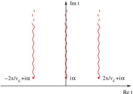
Figure 1: [color online] Branch points and branch cuts for $G_{LL}(t,x,x;\beta)$. The phases are different in different regions defined by branch points.

Functions $G_{LL}(t,x,x;\beta)$ and $G_{LL}(t,x,-x;\beta)$ have different phases in different regions defined by branch points, since the phases differ by $2\pi$ on opposite sides of the cuts. Taking the cutoff $\alpha\rightarrow 0$ we get

$${\rm Re}\,G_{LL}(t,x,x;\beta)=\left(\frac{\pi}{\beta v_{c}}\right)^{k_{1}+k_{2}}\!\!\!\left(\frac{\pi}{\beta v_{s}}\right)^{1/2}\!\!\!\cos\zeta(t)\left|\sinh(\frac{\pi}{\beta}t)\right|^{-(1/2+k_{1}+k_{2})}\left|\frac{\sinh(\frac{\pi}{\beta}(t+\frac{2x}{v_{c}}))\sinh(\frac{\pi}{\beta}(t-\frac{2x}{v_{c}}))}{\sinh^{2}(\frac{\pi}{\beta}\frac{2x}{v_{c}})}\right|^{-k_{3}}\!\!\!\!\!\!\!\!,$$ (31)

$${\rm Re}\,G_{LL}(t,x,-x;\beta)=\left(\frac{\pi}{\beta v_{c}}\right)^{k_{1}+k_{2}}\!\!\!\left(\frac{\pi}{\beta v_{s}}\right)^{1/2}\!\!\!\cos\zeta^{\prime}(t)\left|\sinh(\frac{\pi}{\beta}(t+2x/v_{s}))\right|^{-1/2}\\ \times\left|\sinh(\frac{\pi}{\beta}(t+2x/v_{c}))\right|^{-k_{1}}\left|\sinh(\frac{\pi}{\beta}(t-2x/v_{c}))\right|^{-k_{2}}\left|\frac{\sinh(\frac{\pi}{\beta}t)}{\sinh(\frac{\pi}{\beta}\frac{2x}{v_{c}})}\right|^{-2k_{3}}\!\!\!\!\!\!\!\!\!\!\!,$$ (32)

with $k_{1},k_{2},$ and $k_{3}$ defined in Eq. (III.1), and where

$$\zeta(t) = \left\{\begin{array}[]{ll}\frac{\pi}{4}+\frac{\pi k_{1}}{2}+\frac{\pi k_{2}}{2}&0<t<\frac{2x}{v_{c}}\\ \frac{\pi}{4}+\frac{\pi k_{1}}{2}+\frac{\pi k_{2}}{2}+\pi k_{3}&t>\frac{2x}{v_{c}}\end{array}\right.$$ (35)

$$\zeta^{\prime}(t) = \left\{\begin{array}[]{ll}\frac{\pi}{4}+\frac{\pi k_{1}}{2}+\frac{\pi k_{2}}{2}+\pi k_{3}&t<-\frac{2x}{v_{s}}\\ -\frac{\pi}{4}+\frac{\pi k_{1}}{2}+\frac{\pi k_{2}}{2}+\pi k_{3}&-\frac{2x}{v_{s}}<t<-\frac{2x}{v_{c}}\\ -\frac{\pi}{4}-\frac{\pi k_{1}}{2}+\frac{\pi k_{2}}{2}+\pi k_{3}&-\frac{2x}{v_{c}}<t<0\\ -\frac{\pi}{4}-\frac{\pi k_{1}}{2}+\frac{\pi k_{2}}{2}-\pi k_{3}&0<t<\frac{2x}{v_{c}}\\ -\frac{\pi}{4}-\frac{\pi k_{1}}{2}-\frac{\pi k_{2}}{2}-\pi k_{3}&t>\frac{2x}{v_{c}}\end{array}\right.$$ (41)

We see that the phases that appear in the real parts of the Green’s functions take different values in different domains, consistent with the fact that the end points of the domains are branch points (see Fig. 1). Given the results in Eq. (32) we can finally write down an exact representation of the LSW for an LL with an open boundary. Combining (5) and (19) we find that

$$A(\omega,x,\beta) = \frac{4}{\pi}\int_{0}^{\infty}dt\cos\omega tReG_{LL}(t,x,x;\beta)$$ (42)

$$+ \frac{2}{\pi}\int_{-\infty}^{\infty}dt\cos(2k_{F}x+\gamma-\omega t)Re\,G_{LL}(t,x,-x;\beta).$$

This expression reveals that $A(\omega,x,\beta)$ has a nontrivial dependence on the interaction strength (via $k_{1},k_{2},k_{3}$ and the velocities $v_{c}$ and $v_{s}$ that parameterize the chiral Green’s functions), in addition to an oscillation in the second term that is shifted by a phase controlled by the band filling via $k_{F}$ and $\gamma$ in Eq. (14) and the distance $x$ to the boundary. This leads to an interesting asymmetric dependence of the LSW on energy as will be discussed in Sec. IV.

One of the most promising candidates for LL behavior are single-walled carbon nanotubes (SWCNT), which however require some modification to the Green’s functions in Eqs. (29)-(32) due to the presence of two electronic channels. Depending on the substrate the interaction constant $K_{c}$ may be very small $\approx 0.25$ and strongly k-dependent for isolating substrates or closer to unity $\approx 0.6-1$ for metallic substrates. Especially in the latter case backscattering processes may also play an important role at very low temperatures. Following [EggerGogolinPRL, ; BalentsFisher, ] the low energy expression for the electron field is written in terms of Bloch functions on the two graphite sublattices in order to arrive at two spinful channels of 1D Fermion operators ${\psi}_{L\alpha\sigma}$ and ${\psi}_{R\alpha\sigma}$ where $\sigma=\uparrow,\downarrow$ is the spin and $\alpha=\pm$ labels the two distinct channels. In order to bosonize the problem it is then possible to introduce bosonic fields of total and relative $(\delta=\pm)$ charge and spin chiral bosons $\phi_{rj\delta}\,(r=L,R,\ \ j=c,s)$ and write the bosonization formula

$${\psi}_{L\alpha\sigma}=\frac{\eta_{L\alpha\sigma}}{\sqrt{2\pi\alpha}}\exp(-i\sqrt{\pi}[\cosh\theta\phi_{Lc+}(x)+\sinh\theta\phi_{Rc+}(x)+\alpha\phi_{Lc-}(x)+\sigma\phi_{Ls+}(x)+\alpha\sigma\phi_{Ls-}(x)]),$$ (43)

where ${\psi}_{R\alpha\sigma}$ is obtained by taking the complex conjugate of the right-hand-side of Eq. (43) and switching $L\leftrightarrow R$.

An open end or an impurity will in general mix the two channels so the effective ”open” boundary condition will in most cases not be a simple reflection. The analytic continuation analogous to Eq. (III.1) may therefore turn out to be more complicated for the four bosons. In the simplest symmetric cases we see that the boundary Green’s functions have again a structure as given in Eqs. (29-32), however with the exponent $1/2$ replaced by $3/4$ and $k_{1}=\left(K_{c+}+1/K_{c+}+2\right)/16$, $k_{2}=\left(K_{c+}+1/K_{c+}-2\right)/16$ and $k_{3}=\left(1/K_{c+}-K_{c+}\right)/16$. Accordingly $\zeta(t)$ and $\zeta^{\prime}(t)$ are given by Eq. (35) with each occurrence of the term $\pi/4$ in (35) replaced by $3\pi/8$. The oscillating Friedel-like terms in the LSW in the second term of Eq. (42) turn out to have the opposite sign on the two sublattices mele .

IV Results

In order to extract the physics from the LSWs derived in the previous section we have numerically carried out the Fourier transforms in Eq. (42). The results reveal a rich structure in the LSW of a Luttinger liquid when an edge or an impurity is present. We here focus on three aspects of the LSW of particular interest for STM experiments: Its asymmetric line shape as a function of energy, oscillation patterns revealing spin-charge separation, and thermal effects. To keep the discussion general, we do not specify the dependence of the velocities $v_{c,s}$ on the Luttinger liquid parameter $K_{c}$, which is sensitive to the choice of microscopic model. Since our results do not depend on the particular relation between $v_{c,s}$ and $K_{c}$, we choose them freely so as to be able to observe all possible scenarios for the behavior of the LSW. The question whether a particular scenario will be realized in a particular model is of course determined by the relation between velocities and Luttinger liquid parameter.

IV.1 Properties of the LSW

One of the most striking feature of the LSW of an LL is the well-known power law suppression at low energies proportional to $\omega^{(K_{c}+K_{c}^{-1})/4-1/2}$. For the special case of zero temperature and commensurate oscillations (i.e. setting $2k_{F}na+\gamma=\pi m\,(m\in{\mathbb{Z}})$) the LSW of Eq. (42) near a boundary at $x=na$ has been analyzed before EJM ; Eggert . In that case the first term of Eq. (42) takes on a scaling form with the variable $\omega x$ that shows a crossover from bulk scaling to boundary scaling in Eq. (1) with slow oscillations proportional to $\sin(2\omega x/v_{c})\omega^{k_{3}-1}x^{k_{3}-k_{1}-k_{2}-1/2}$ EJM . If the phase is neglected or set to $2k_{F}na+\gamma=m\pi$ the second Friedel-like term in Eq. (42) also takes on a scaling form, but shows both spin and charge modulations that decay with $\omega^{k_{1}-1}x^{-k_{2}-1/2}$. We will now focus on the energy dependence at both small and large temperatures together with the effect of the phase $\gamma$.

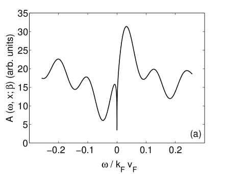
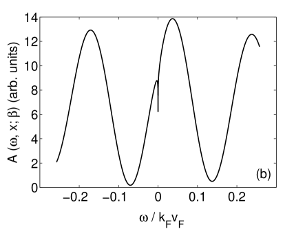
Figure 2: Local spectral weight $A(\omega,x;\beta)$ for $K_{c}=0.7$, $v_{c}/v_{F}\approx 1.43$, $v_{c}/v_{s}\approx 3$ (a), $K_{c}=0.9$, $v_{c}/v_{F}\approx 1.11$, $v_{c}/v_{s}\approx 1.26$ (b) with $T/k_{F}v_{F}=2.6\times 10^{-6}$, $x=10a$, $n_{e}=0.97$.

IV.1.1 Asymmetric line-shape

At small energies, the most striking feature of the LSW is the asymmetry of its line shape, as seen in Fig. 2. From Eq. (42) it is apparent that this property is due to the phase $2k_{F}x+\gamma$ appearing in the second term of $A(\omega,x;\beta)$. Here the distance from the boundary $x=na$ has to be measured in integer units of the lattice spacing $a$, since the original Fermion operators typically correspond to orbitals in the crystal lattice. The phase causes a shift of the periodic structure of $A(\omega,x;\beta)$ with respect to the Fermi level, and accordingly determines how the spectral weight suppression close to the Fermi level affects the line shape.

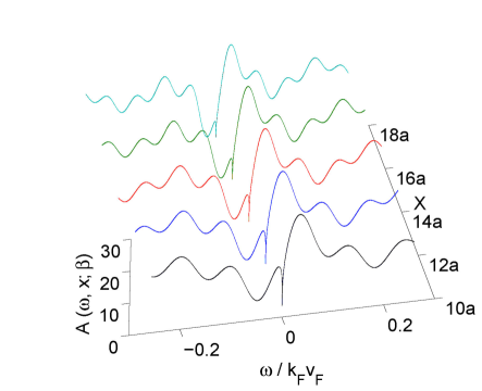
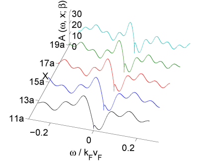
Figure 3: [color online] $A(\omega,x;\beta)$ for $K_{c}=0.7$, $v_{c}/v_{F}\approx 1.43$, $v_{c}/v_{s}\approx 3$, $T/k_{F}v_{F}=2.6\times 10^{-6}$, $n_{e}=0.97$, shown for even and odd sublattices.

The shift depends upon the filling factor $n_{e}$ since, for fixed $x$, $n_{e}$ determines the values of $k_{F}$ and $\gamma$ in Eq. (14). The LSW is asymmetric in general, but for particular fillings for which $2k_{F}na+\gamma=\pi m\,(m\in{\mathbb{Z}})$ it becomes a symmetric function of $\omega$. By inspection of Eqs. (32) and (42) one finds that for a given interaction strength the asymmetry tends to zero very close to the boundary ($2\omega x/v_{s}\ll 1$) and very far from the boundary ($2\omega x/v_{c}\gg 1$, ”bulk” regime) and reaches a maximum in the intermediate region. It is important to realize that the shift of the periodic structure with respect to the Fermi level is present also for the non-interacting case when the LSW takes the simple form $A(\omega,x;\beta)\sim\cos(2k_{F}x+\gamma-2\omega x/v_{F})$. We conclude that the shift is a pure boundary effect, and is due to the interference of the incoming and reflected electrons at the boundary. In contrast, the dip of the spectral weight at the Fermi level is an interaction effect.

In Fig. 3 we show the energy and coordinate dependence of the LSW for even and odd sublattices. The Friedel oscillations on the scale of the lattice spacing $a$ are easily visible as a flip of the asymmetry when going from one graph to the other. The spin and charge modulations of the amplitude are also present over longer wavelengths in real space, but are not clearly visible due to the relatively narrow coordinate range in Fig. 3. Note that the asymmetry with energy varies with the distance to the boundary since the phase $2k_{F}x+\gamma$ also varies with distance.

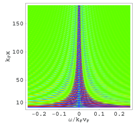
Figure 4: [color online] $A(\omega,x;\beta)$ for $K_{c}=0.7$, $v_{c}/v_{F}\approx 1.43$, $v_{c}/v_{s}\approx 3$, $T/k_{F}v_{F}=2.6\times 10^{-4}$, $n_{e}=0.97$.

It is interesting to note the similarity of the typical asymmetric line shapes in Figs. 2 and 3 with that of a Fano resonance Fano when $\omega$ is close to the Fermi level. A Fano resonance is known to develop in the LSW for non-interacting electrons when coupled e.g. to a magnetic impurity, the effect being produced by the interference between resonating and nonresonating electron paths through the impurity Ujsaghy . As we have seen, the asymmetry in the present case instead comes from the combined effect of electron interactions (causing a dip in the LSW at the Fermi level) and the reflection of electrons off the boundary (causing a phase shifted oscillation in the LSW). As one expects the Fano line shape to survive for interacting electrons coupled to a magnetic impurity it is indeed satisfying to see this feature reproduced by the open boundary for which the impurity gets traded at low temperatures.

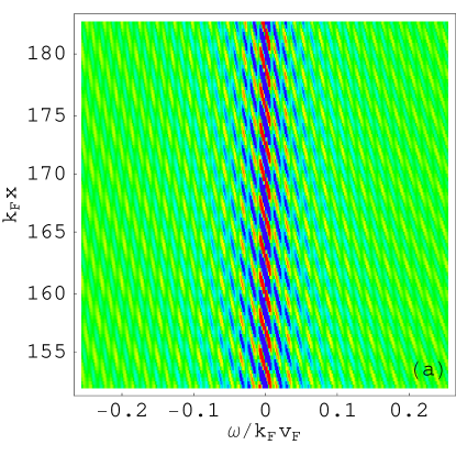
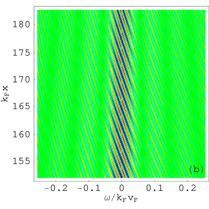
Figure 5: [color online] $A(\omega,x;\beta)$ for $T/k_{F}v_{F}=2.6\times 10^{-6}$, $n_{e}=0.97$, with $K_{c}=0.7$, $v_{c}/v_{F}\approx 1.43$, $v_{c}/v_{s}\approx 3$ (a) and $K_{c}=0.9$, $v_{c}/v_{F}\approx 1.11$, $v_{c}/v_{s}\approx 1.26$ (b). The color coding is the same as in Fig. 4.

IV.1.2 Spin-charge separation

The proximity to an open boundary reveals a key property of interacting electrons in one dimension $-$ spin-charge separation $-$ i.e. the fact that the collective spin and charge excitations (induced e.g. by inserting an extra electron into the system), propagate with different speeds, and hence ”separate” Voit . The effect shows up in the LSW as a characteristic peak structure at intermediate distances from the boundary. Very far from the boundary ($\omega x_{s}\gg 1$) $A(r,\omega;\beta)$ is a monotone function scaling as $\omega^{\alpha}$ near the Fermi level, with bulk exponent $\alpha=(K_{c}+K_{c}^{-1})/4-1/2$ at low temperatures Voit . Extremely close to the boundary ($\omega x_{s}\ll 1$) $A(r,\omega;\beta)$ has a similar structure, but with an enhanced suppression near the Fermi level, $A(r,\omega;\beta)\sim\omega^{\alpha_{B}}$, with boundary exponent $\alpha_{B}=(K_{c}^{-1}-1)/2$ at low temperatures KaneFisher ; FabrizioGogolin ; EJM (see Fig. 4, with color coding in arbitrary units). As one moves away from the immediate vicinity of the boundary an oscillation pattern emerges, which becomes most pronounced when $\omega x_{s}\sim{\cal O}(1)$. This oscillatory feature (see Fig. 5) which is a superposition of spin and charge waves is due to the two types of branch points in Eqs. (29) and (30) which define the propagating collective spin and charge modes. The two panels correspond to two different choices of $K_{c}$, with two different values of the ratio $v_{c}/v_{s}$, leading to the two different peak structures. By close inspection of the graphs one can easily read off the corresponding velocity ratios. To see how, let us make a ”cut” of the two panels in Fig. 5 at a distance $x=100a$ from the boundary, yielding the panels in Fig. 6.

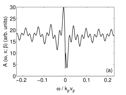
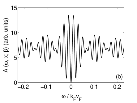
Figure 6: $A(\omega,x;\beta)$ for $T/k_{F}v_{F}=2.6\times 10^{-6}$, $n_{e}=0.97$, with $x=50a$, $K_{c}=0.7$, $v_{c}/v_{F}\approx 1.43$, $v_{c}/v_{s}=\lambda_{c}/\lambda_{s}\approx 3$ (a) and $x=100a$, $K_{c}=0.9$, $v_{c}/v_{F}\approx 1.11$, $v_{c}/v_{s}=\lambda_{c}/\lambda_{s}\approx 1.26$ (b).

When $K_{c}=0.7$ (panel (a)) the spin and charge velocities differ significantly. For this case the short wavelength ($\lambda_{s}=\pi v_{s}/x$) spin oscillations are modulated by long wavelength charge oscillations ($\lambda_{c}=\pi v_{c}/x$). We note that there are three spin oscillations per one charge oscillation which is in agreement with the fact that in this case $\lambda_{c}/\lambda_{s}=v_{c}/v_{s}\approx 3$ (see Fig. 6 (a)). When $K_{c}$ gets closer to unity (non-interacting limit) the spin and charge velocities approach each other and the spin-charge separation manifests itself as a beating pattern, provided that $K_{c}$ is not identical to unity (see Fig. 6 (b) where $K_{c}=0.9$). The short wavelength ($\lambda=2\pi v_{s}v_{c}/x(v_{s}+v_{c})$) oscillations are now amplitude modulated by long wavelength oscillations ($\lambda^{\prime}=2\pi v_{s}v_{c}/x(v_{c}-v_{s})$). We see that there are about six short wavelength oscillations per ”bubble” of the long wavelength amplitude modulations, which is in agreement with the fact $\lambda^{\prime}/\lambda\approx 12$ in this case, corresponding to $\lambda_{c}/\lambda_{s}=v_{c}/v_{s}\approx 1.26$.

The spin-charge oscillations in the LSW are also present in real space as discussed before Eggert . The oscillations as a function of energy might be easier to observe, however, since here there are no superimposed Friedel oscillations. We also remark that the existence of the beating pattern for values of $K_{c}$ close to unity was proposed in Ref. [UssishkinGlazman, ] as a diagnostic tool for spin-charge separation in possible tunneling experiments of an LL where a scanning probe microscopy tip would be used as an impurity.

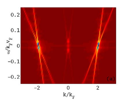
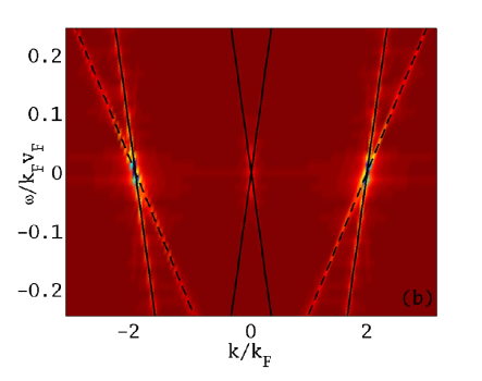
Figure 7: Fourier transform of the LSW for $K_{c}=0.7$, $v_{c}/v_{F}\approx 1.43$, $v_{c}/v_{s}\approx 3$, $T/k_{F}v_{F}=2.6\times 10^{-4}$, $n_{e}=0.97$ (a) and the same graph with charge (solid lines) and spin (dashed lines) wave dispersions superimposed (b).

One can map the dispersion of the spin and charge waves by taking a Fourier transform of the LSW (see Fig. 7 (a)). This Fourier transform should not be confused with the momentum or angle resolved spectral weight, which is measured in photoemission experiments, although it shows similar features of spin charge separation. The dominant weights in the transform correspond to the $\omega(k)$ dependence of the excitations. The dispersion lines at $k=0$ come from the non-oscillatory part of the LSW and represent the charge excitations, since the non-oscillatory part contains only charge oscillations. This feature at $k=0$ is also a clear indication of interaction effects and disappears as $K_{c}\to 1$. The dispersion lines at $k\neq 0$ come from the Friedel terms, and contain spin and charge branches shifted from $k=0$ by $\pm 2k_{F}$. The mirror symmetry about $k=0$ reflects the standing wave nature of the oscillations. In Fig. 7 (b) the dispersion relations $\omega(k)=\pm kv_{c}/2$ at $k\approx 0$ and $\omega(k)=(\pm k-2k_{F})v_{c/s}/2$ at $k\approx\pm 2k_{F}$ are plotted on top of the Fourier transform and agree with the location of the maxima.

IV.1.3 Thermal effects

On general grounds one expects that thermal effects become visible only for energies $\omega\lesssim T$ and distances $x\gtrsim\lambda_{T}=v_{s}/T$. Choosing e.g. $T\lesssim 10$K and $v_{F}\approx 10^{5}\rm m/s$ (a typical value for a quasi-1D organic metal for which LL theory should be applicable Giamarchi ) this implies that the spin-charge peak structure as seen in Fig. 5 will remain intact for distances not too far from the edge ($2x/\beta v_{s}\ll 1$). We should caution the reader that the energy range for which the LL theory is applicable to a specific experiment may sometimes be smaller than the range depicted in Fig. 5 (cf. our discussion in Sec. I). For $2x/\beta v_{c}\gtrsim 1$ the spin and charge waves loose their coherence before reaching the edge and therefore spin-charge separation is destroyed (see Fig. 9(a)).

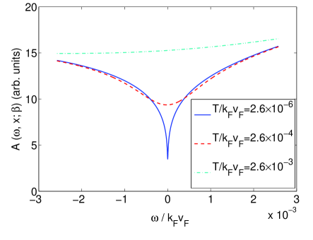
Figure 8: [color online] $A(\omega,x;\beta)$ for $K_{c}=0.7$, $v_{c}/v_{F}\approx 1.43$, $v_{c}/v_{s}\approx 3$, $x=10a$, $n_{e}=0.97$ at different temperatures.

A more interesting issue is the fate of the asymptotic scaling behavior of the LSW near the Fermi level as the temperature increases. In earlier work it was found that the ”uniform part” of the LSW (corresponding to the first term in (42) crosses over to $\omega^{2}$ scaling in both boundary ($2\omega x/v_{s}\ll 1$) and bulk regimes ($2\omega x/v_{c}\gg 1$) when $\omega\beta<1$ MEJ . The effect was found to originate in the exponential damping of the density correlations for unequal times due to thermal fluctuations. By performing an expansion of the full LSW in Eq. (42) with the small parameter $\omega\beta$ we find that the power law is now modified to

$$A(\omega,x;\beta)\sim A+B\omega+C\omega^{2},\ \ \ \ \omega\beta\ll 1$$ (44)

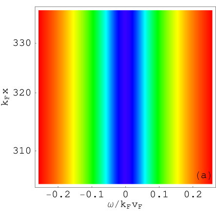
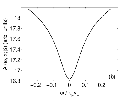
Figure 9: [color online] $A(\omega,x;\beta)$ for $T/k_{F}v_{F}=2.6\times 10^{-2}$, $K_{c}=0.7$, $v_{c}/v_{F}\approx 1.43$, $v_{c}/v_{s}\approx 3$, $n_{e}=0.97$ (a) and cut at $x=200a$ (b).

where $A,B$ and $C$ depend on the temperature and the distance from the boundary. We depict the crossover from boundary scaling $\sim\omega^{(K_{c}^{-1}-1)/2}$ for $\omega\beta\gg 1$ to thermal scaling $\sim A+B\omega+C\omega^{2}$ for $\omega\beta\ll 1$ in Fig. 8. Note that one is able to observe this crossover for $2x/\beta v_{s}\ll 1$. For $2x/\beta v_{c}\gtrsim 1$ the boundary scaling is completely washed out. Since in this regime $G_{LL}(t,x,-x;\beta)$ in Eq. (30) is exponentially suppressed compared to $G_{LL}(t,x,x;\beta)$ in (29), it follows that $A(\omega,x;\beta)\sim A+C\omega^{2}$, and the line shape becomes symmetric (see Fig. 9b).

In this context it is important to point out that our finite-temperature results are strictly valid only for the case where an edge is modeled by an open boundary. An impurity, on the other hand, is faithfully represented by an open boundary condition only in the zero-temperature limit KaneFisher ; FurusakiNagaosa1 . For finite temperatures a new energy scale $T_{0}$ appears, characterizing the crossover from weak to strong coupling (”open boundary fixed point”), and depending on the impurity strength $V_{0}$. A simple RG estimate shows that $T_{0}$ scales with $V_{0}$ as $T_{0}\sim V_{0}^{2/(1-K_{c})}$, with an overall scale factor that depends on the details of the regularization procedure FurusakiNagaosa1 . For finite $T$ with $T\ll T_{0}$, an open boundary representation of the impurity is still expected to capture the essential physics. An interesting, albeit technically challenging project would be to redo the calculations in this section for an impurity in the presence of the operators that appear away from the $T=0$ open boundary fixed point, allowing for a complete picture of impurity thermal effects.

IV.2 Properties of the Local Tunneling Conductance

The local differential tunneling conductance, defined in Eq. (9), exhibits the very same features as the LSW. The only difference is that the fine structure of the differential conductance is thermally smeared via the temperature dependence of the Fermi-Dirac distribution. This can clearly be seen by examining the energy dependence at some fixed distance from the boundary, as done in Fig. 10, and then comparing to the corresponding graphs for the LSW in Fig. 6. As the smearing occurs on the scale of $T$, spin-charge separation is wiped out for temperatures $T\gtrsim\lambda_{s}$. The distance $x$ from the boundary determines the wavelength of the oscillations in energy space, so in most cases it should be possible to find a range for $x$ which shows many waves in the energy interval where LL theory applies that are not washed out by temperature, i.e. $1/\Delta\ll x/v_{c}\ll 1/T$, where $\Delta$ is the bandwidth. Note that the inequality above coincides with the criterion for observing spin-charge separation in the LSW, discussed in the previous subsection.

In wires of finite length $l$ the energy levels become discrete and are given by a characteristic direct product of two spectra with uniform spacing $\pi v_{c}/l$ and $\pi v_{s}/l$ MEJ ; AnfusoEggert . The standing waves of the individual levels show the corresponding intereference of spin and charge excitations AnfusoEggert . If the temperature becomes comparable to the level spacing, a continous pattern of Friedel oscillations as shown above emerges. However, in order to see the predicted behavior at all, the wire must always be long enough so that many levels lie within the energy interval in which the LL theory applies, i.e. $\pi v_{c}/l\ll\Delta$. For metallic materials this translates into lengths of typically 100nm or more.

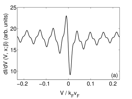
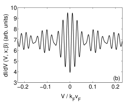
Figure 10: $dI/dV(V,x;\beta)$ for $T/k_{F}v_{F}=2.6\times 10^{-3}$, $n_{e}=0.97$, with $x=50a$, $K_{c}=0.7$, $v_{c}/v_{F}\approx 1.43$, $v_{c}/v_{s}=\lambda_{c}/\lambda_{s}\approx 3$ (a) and $x=100a$, $K_{c}=0.9$, $v_{c}/v_{F}\approx 1.11$, $v_{c}/v_{s}=\lambda_{c}/\lambda_{s}\approx 1.26$ (b).

When applying the results to SWCNTs similar features can be expected as has already been partially confirmed experimentally Lee . The dominant effect is the complicated interference pattern of the Bloch waves, which strongly depends on the geometry of the boundary condition and the chirality of the tubes mele . Nonetheless, an enhanced velocity, a suppressed spectral weight and a characteristic power law of decaying oscillations are clear signatures of interaction effects which all have been seen in experiments Lee . A more complete theoretical analysis would also have to include the effects of backscattering, band structure, longer-range interactions and the mixing of the channels near the boundary which we defer to a future publication.

V Summary

We have derived the full finite-temperature LSW for a Luttinger liquid with an edge or impurity (modeled as an open boundary condition), relevant to high-precision STM measurements. We have also generalized our approach to the ”two-channel” case that describes SWCNTs in the Luttinger liquid regime, which is qualitatively similar to the single-channel case.

The LSW (determining the local differential tunneling conductance in STM measurements) exhibits a very rich structure as a function of temperature, distance from the impurity, and the strength of the electron interaction. Depending on the choice of parameters one is able to see asymmetric Fano-like line shapes and spin and charge oscillations. The Fano-like asymmetries are caused by an interplay of boundary and interaction effects, and, as we have shown, are closely linked to the Friedel oscillations in real space. Spin and charge oscillations appear due to the interference of propagating spin and charge waves reflected from the boundary.

We have discussed how to consistently determine the key parameters of a Luttinger liquid (the interaction parameter $K_{c}$, and the spin and charge velocities) from experimental measurements of the tunneling conductance. We have also extensively discussed various thermal effects with focus on their influence on the Fano-like asymmetries and spin-charge oscillations in the LSW as a function of energy. The thermal suppression of the coherence of spin and charge waves makes it hard to detect interaction effects in the LSW and even more so in the local differential tunneling conductance (where the finite-temperature LSW gets weighted by the Fermi-Dirac distribution): For temperatures $T\gtrsim v_{s}/x$ (where $v_{s}$ is the speed of the spin excitations, and $x$ is the distance to the edge or the impurity) the characteristic power law behavior near the Fermi level is completely washed out and replaced by an interaction-independent analytic scaling. For these temperatures spin-charge separation also becomes virtually impossible to detect.

In conclusion, our results provide guidelines for identifying and interpreting signals of electron correlations in STM data on SWCNTs and other one-dimensional systems, and as such should be useful in the search for realizations of Luttinger liquid physics.

- (1) T. Giamarchi, Quantum Physics in One Dimension (Oxford University Press, Oxford, 2004).
- (2) J. Voit, Rep. Prog. Phys. 58, 977 (1995).
- (3) C. L. Kane and M. P. A. Fisher, Phys. Rev. B 46, 15233 (1992).
- (4) A. Furusaki and N. Nagaosa, Phys. Rev. B 47, 4631 (1993).
- (5) A. Furusaki and N. Nagaosa, Phys. Rev. Lett. 72, 892 (1994).
- (6) S. Eggert and I. Affleck, Phys. Rev. B 46, 10866 (1992).
- (7) M. Fabrizio and A.O. Gogolin, Phys. Rev. B 51, 17827 (1995).
- (8) S. Eggert, H. Johannesson, and A. Mattsson, Phys. Rev. Lett. 76, 1505 (1996).
- (9) A. E. Mattsson, S. Eggert, and H. Johannesson, Phys. Rev. B 56, 15615 (1997).
- (10) J. Voit, Y. Wang, and M. Grioni, Phys. Rev. B 61, 7930 (2000).
- (11) Y. Wang, J. Voit, and F.-C. Pu, Phys. Rev. B 54, 8491 (1996).
- (12) F. Anfuso and S. Eggert, Phys. Rev. B 68, 241301(R) (2003).
- (13) K. Schönhammer, V. Meden, W. Metzner, U. Schollwöck, and O. Gunnarsson, Phys. Rev. B 61, 4393 (2000).
- (14) V. Meden, W. Metzner, U. Schollwöck, O. Schneider, T. Stauber, and K. Schönhammer, Eur. Phys. J. B 16, 631 (2000).
- (15) M. Bockrath, D. H. Cobden, H. Lu, A. G. Rinzler, R. E. Smalley, L. Balents, and P. L. McEuen, Nature 397, 598 (1999).
- (16) A. Yacoby, H. L. Stormer, N. S. Wingreen, L. N. Pfeiffer, K. W. Baldwin, and K. W. West, Phys. Rev. Lett. 77, 4612 (1996).
- (17) P. Segovia, D. Purdie, M. Hengsberger, and Y. Baer, Nature 402, 504 (1999).
- (18) S. Eggert, Phys. Rev. Lett. 84, 4413 (2000).
- (19) S. A. Kivelson, I. P. Bindloss, E. Fradkin, V. Oganesyan, J. M. Tranquada, A. Kapitulnik, and C. Howald, Rev. Mod. Phys. 75, 1201 (2003).
- (20) Note that the boundary exponent in Ref. [EJM, ] is expressed via a non-standard parameterization of the LL interaction.
- (21) Z. Yao, H. W. Ch. Postma, L. Balents, and C. Dekker, Nature 402, 273 (1999).
- (22) O. M. Auslaender, A. Yacoby, R. de Picciotto, K. W. Baldwin, L. N. Pfeiffer, and K. W. West, Science 295, 825 (2002).
- (23) F. Zwick, S. Brown, G. Margaritondo, C. Merlic, M. Onellion, J. Voit, and M. Grioni, Phys. Rev. Lett. 79, 3982 (1997).
- (24) For a review, see O. Gunnarsson, K. Schönhammer, J. W. Allen, K. Karlsson, and O. Jepsen, J. Electr. Spectr. 117, 1 (2001).
- (25) An alternative setup which avoids this problem is to use the scanning tip to create a local potential with a scanning probe microscopy tip which scatters electrons, and then measure how the tunneling into the system from a fixed tunnel junction depends on the distance from the tip position as suggested by Ref. [UssishkinGlazman, ].
- (26) L. C. Venema, J. W. G. Wildoer, J. W. Janssen, S. J. Tans, H. L. J. T. Tuinstra, L. P. Kouwenhoven, and C. Dekker, Science 283, 52 (1998).
- (27) S. G. Lemay, J. W. Janssen, M. van den Hout, M. Mooij, M. J. Bronikowski, P. A. Willis, R. E. Smalley, L. P. Kouwenhoven, and C. Dekker, Nature 412, 617 (2001).
- (28) B. J. LeRoy, S. G. Lemay, J. Kong, and C. Dekker, Appl. Phys. Lett. 84, 4280 (2004)
- (29) J. Lee, H. Kim, S.-J. Kahng, G. Kim, Y.-W. Son, J. Ihm, H. Kato, Z. W. Wang, T. Okazaki, H. Shinohara, and Y. Kuk, Nature (London) 415, 1005 (2002).
- (30) J. Lee, S. Eggert, H. Kim, S. J. Kahng, H. Shinohara, and Y. Kuk, Phys. Rev. Lett. 93, 166403 (2004).
- (31) K. Penc, K. Hallberg, F. Mila, and H. Shiba, Phys. Rev. Lett. 77, 1390 (1996); Phys. Rev. B 55, 15475 81997).
- (32) V. Meden, W. Metzner, U. Schollwöck, and K. Schönhammer, Phys. Rev. B 65, 045318 (2002).
- (33) R. Egger and A. O. Gogolin, Eur. Phys. J. B 3, 281 (1998).
- (34) U. Fano, Nuovo Cimento 12, 156 (1935); Phys. Rev. 124, 1866 (1961).
- (35) O. Újsághy, J. Kroha, L. Szunyogh, and A. Zawadowski, Phys. Rev. Lett. 85, 2557 (2000).
- (36) G. Rickayzen, Green’s Functions and Condensed Matter (Academic Press, London, 1980).
- (37) J. Tersoff and D. R. Hamann, Phys. Rev. B 31, 805 (1985).
- (38) A. O. Gogolin, A. A. Nersesyan, and A. M. Tsvelik, Bosonization and Strongly Correlated Systems (Cambridge University Press, Cambridge, 1998).
- (39) H. J. Schulz, Phys. Rev. Lett. 71, 1864 (1993).
- (40) P. Di Fransesco, P. Mathieu, and D. Senechal, Conformal Field Theory (Springer Verlag, New York, 1997).
- (41) G. Mahan, Many-Particle Physics (Plenum, New York, 1981).
- (42) R. Egger and A. O. Gogolin, Phys. Rev. Lett. 79, 5082 (1997).
- (43) L. Balents and M. P. A. Fisher, Phys. Rev. B 55, R11973 (1997).
- (44) C.L. Kane and E.J. Mele, Phys. Rev. B 59, R12759 (1999).
- (45) I. Ussishkin and L. I. Glazman, Phys. Rev. Lett. 93, 196403 (2004).