Effect of DC electric field on longitudinal resistance of two dimensional electrons in a magnetic field.

Abstract

The effect of a DC electric field on the longitudinal resistance of highly mobile two dimensional electrons in heavily doped GaAs quantum wells is studied at different magnetic fields and temperatures. Strong suppression of the resistance by the electric field is observed in magnetic fields at which the Landau quantization of electron motion occurs. The phenomenon survives at high temperature where Shubnikov de Haas oscillations are absent. The scale of the electric fields essential for the effect is found to be proportional to temperature in the low temperature limit. We suggest that the strong reduction of the longitudinal resistance is the result of a nontrivial change in the distribution function of 2D electrons induced by the DC electric field. Comparison of the data with recent theory yields the inelastic electron-electon scattering time $\tau_{in}$ and the quantum scattering time $\tau_{q}$ of 2D electrons at high temperatures, a regime where previous methods were not successful.

The nonlinear properties of highly mobile two dimensional electrons in AlGaAs/GaAs heterojunctions is a subject of considerable current interest. Strong oscillations of the longitudinal resistance induced by microwave radiation have been found at magnetic fields which satisfy the condition $\omega=n\times\omega_{c}$, where $\omega$ is the microwave frequency, $\omega_{c}$ is cyclotron frequency and $n$=1,2…zudov ; engel . At high levels of the microwave excitations the minima of the oscillations can reach values close to zero mani ; zudov2 ; dorozh1 ; willett . This so-called zero resistance state (ZRS) has stimulated extensive theoretical interest andreev ; durst ; anderson ; shi ; vavilov ; dmitriev . At higher magnetic field $\omega_{c}>\omega$ a considerable decrease of magnetoresistance with microwave power is found engel ; dorozh1 ; willett which has been attributed to intra-Landau-level transitionsdorozh2 .

Another interesting nonlinear phenomenon has been observed in response to DC electric field yang ; bykov1 . Oscillations of the longitudinal resistance, which are periodic in inverse magnetic field, have been found at DC biases, satisfying the condition $n\times\hbar\omega_{c}=2R_{c}E_{H}$, where $R_{c}$ is the Larmor radius of electrons at the Fermi level and $E_{H}$ is the Hall electric field induced by the DC bias in the magnetic field. The effect has been attributed to ”horizontal” Landau-Zener tunneling between Landau levels, tilted by the Hall electric field $E_{H}$ yang .

In this paper we report a new phenomenon. We have observed a strong reduction of the 2D longitudinal resistance induced by DC electric field $E_{dc}$ which is substantially smaller that required for the ”horizontal” electron transitions between Landau levelsyang ; bykov1 . In contrast to the inter Landau level scattering, the observed effect depends strongly on temperature. We suggest that the phenomenon is due to a substantial and nontrivial deviation of the electron distribution function from equilibrium induced by the DC electric field $E_{dc}$. We find reasonable agreement between our results and a recent theory that considers such an effect in the high temperature limitdmitriev .

Our samples were cleaved from a wafer of high-mobility GaAs quantum well grown by molecular beam epitaxy on semi-insulating (001) GaAs substrates. The width of the GaAs quantum well was 13 nm. AlAs/GaAs type-II superlattices served as barriers, making possible a high-mobility 2D electron gas with high electron density fried . Two samples (N1 and N2) were studied with electron density $n_{1}$ = 1.22 $\times 10^{16}$ m^-2, $n_{2}$ = 0.84 $\times 10^{16}$ m^-2,and mobility $\mu_{1}$= 93 m²/Vs, $\mu_{2}$= 68 m²/Vs at T=2.7K. Measurements were carried out between T=1.8 K and T=77 K in magnetic field up to 3.2 T on $d$=50 $\mu m$ wide Hall bars with a distance of 250 $\mu m$ between potential contacts. The longitudinal resistance was measured using a current of 0.5 $\mu$A at a frequency of 77 Hz in the linear regime. Direct electric current (bias) was applied simultaneously with AC excitation through the same current leads (see insert to fig. 1). Although we have studied, strictly speaking, the differential resistance, for the sake of simplicity we will refer to it below as resistance.

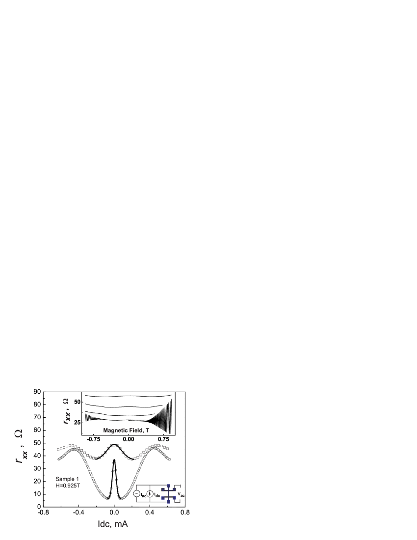
Figure 1: Dependence of the differential resistance $r_{xx}$ on DC bias at H=0.925T. Cirles correspond to T=4.3 K, squares correspond to T=19.8 K. The solid lines are theoretical curves obtained from Eq. 3. The fitting parameters are $I_{0}$=0.055 (mA) and $\delta$=0.334 for T=4.3K and $I_{0}$=0.1802 (mA) and $\delta$=0.177 for T=19.8 K. The top inset shows quantum oscillations of the longitudinal resistance at different temperatures T=1.9 K (bottom curve, right), 4.2 K (bottom curve, left), 9.9, 19.8 and 35 K (remaining curves in ascending order). The experimental set-up is shown at bottom right.

Typical curves of the longitudinal resistance $r_{xx}$ as a function of the DC bias are shown in Fig. 1 at two temperatures. At high DC bias the resistance exhibits maxima that satisfy the condition $n\times\hbar\omega_{c}=2R_{c}E_{H}$, corresponding to ”horizontal” transitions between Landau levelsyang ; bykov1 . Another striking feature is the sharp peak at zero DC bias which broadens as the temperature is raised. This zero bias peak is the main topic of our paper.

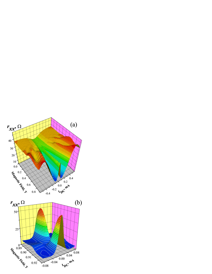
Figure 2: (a) The differential resistance $r_{xx}$ as a function of magnetic field and DC bias at temperature T=4.3 K. (b) A similar plot at T=1.9 K over a narrower range of the experimental parameters, yielding better resolution.

The evolution of the magnetoresistance with DC bias and magnetic field is shown in Fig. 2. The zero bias peak appears at relatively high magnetic field $H\approx 0.2-0.3$ T (see fig.2a). At these fields the Landau level width $\hbar/\tau_{q}$ extracted from amplitude of Shubnikov de Haas (SdH) oscillations becomes to be comparable with $\hbar\omega_{c}$ and the SdH oscillations are visible at low temperatures (see curve at T=1.9K in the top insert to fig.1). The strength of the peak increases gradually with magnetic field. At the zero bias considerable SdH oscillations are present in high magnetic field. The magnitude of the SdH oscillations at T=4.3 K is substantially smaller than the amplitude of the zero bias peak. The peak is still present at temperatures above T=30K where no SdH oscillations are detected. A better resolved snapshot of the peak evolution is presented in Fig. 2b. The figure demonstrates the effect at low temperatures T=1.9 K, where the SdH oscillations are well developed.

The striking reduction of the resistance by several times is observed at temperatures at which no SdH oscillations are present. This is quite different from what one expects for electron heating by the electric field. As shown in the insert to Fig. 1, the resistance increases for higher temperatures, in contrast with the observed decrease with applied electric field. It should also be noted that at low temperatures, the largest effect possible due to heating is to reduce the resistance from its value at a SdH maximum to the ”average” baseline value (which is $\approx$26-28 ($\Omega$) in the insert to Fig. 1). The observed reduction in Fig. 2b is much greater than this indicating a new phenomenon associated with the application of an electric fieldresistance .

From a theoretical perspective, nonlinear phenomena in high mobility 2D electron systems can be conveniently separated into: (a) effects of electric field on the electron distribution function dmitriev , and (b) effects of electric field on the kinematics of electron scattering durst ; vavilov . It was recently realized that the the first of these should provide the dominant contribution to the nonlinear response in 2D electron systems. Below we will compare our results with this approach.dmitriev

The theory considers 2D electrons in classically strong magnetic field at finite electric field $E_{dc}$ and at relatively high temperature $T\gg\hbar\omega_{c}$. Due to conservation of total electron energy $\epsilon+eE_{dc}x$ in the DC electric field $E_{dc}$, the spatial electron diffusion translates into the diffusion of the electrons in energy space. The solution of the diffusion equation in $\epsilon$-space yields nontrivial oscillations of the nonequilibrium electron distribution function with period $\hbar\omega_{c}$. The amplitude of the oscillations is stabilized by inelastic electron-electron scattering, which is found to be proportional to $T^{2}$. Relative to the Drude conductivity, $\sigma_{D}$, in zero magnetic field, the theory predicts a longitudinal conductivity:

$$\Delta\sigma_{xx}/\sigma_{D}=2\delta^{2}[1-\frac{4Q_{dc}}{1+Q_{dc}}],$$

where $\delta=exp(-\pi/\omega_{c}\tau_{q})$ is the Dingle factor, $\tau_{q}$ is the quantum scattering time and the parameter $Q_{dc}$ is

$$Q_{dc}=\frac{2\tau_{in}}{\tau_{tr}}(\frac{eE_{dc}v_{F}}{\omega_{c}})^{2}(\frac{\pi}{\hbar\omega_{c}})^{2}.$$

Here $\tau_{in}$ is the inelastic relaxation time, $\tau_{tr}$ is the transport scattering time and $v_{F}$ is the Fermi velocity.

In order to compare with experiment, the differential conductivity at frequency $\omega$, $\sigma_{\omega}=dJ/dE=d(\sigma(E)E)/dE$, is obtained using eq.(1), and the variation of the differential resistance is found to be:

$$\Delta r_{xx}/R_{0}=2\delta^{2}[\frac{1-10Q_{dc}-3Q_{dc}^{2}}{(1+Q_{dc})^{2}}],$$

where $R_{0}$ is the resistance at zero magnetic field. In a classically strong magnetic field $\omega_{c}\tau_{tr}\gg 1$, the DC electric field is almost perpendicular to the electric current $I_{dc}$: $E_{dc}=\rho_{xy}I_{dc}/d$, where $d$ is the sample width. Using Eq. 2, we rewrite the parameter $Q_{dc}$ in the form $Q_{dc}=(I_{dc}/I_{0})^{2}$, where the scale $I_{0}$ is a fitting parameter. In accordance with Eq. 3 the parameter $I_{0}$ is directly related to the width of the zero bias peak and the peak magnitude is proportional to $\delta^{2}$. Below we refer to the parameter $I_{0}$ as the linewidth. Examples of theoretical fits to the data using Eq.3 are shown by the solid lines in Fig. 1, using $\delta$ and $I_{0}$ as fitting parameterscomparison .

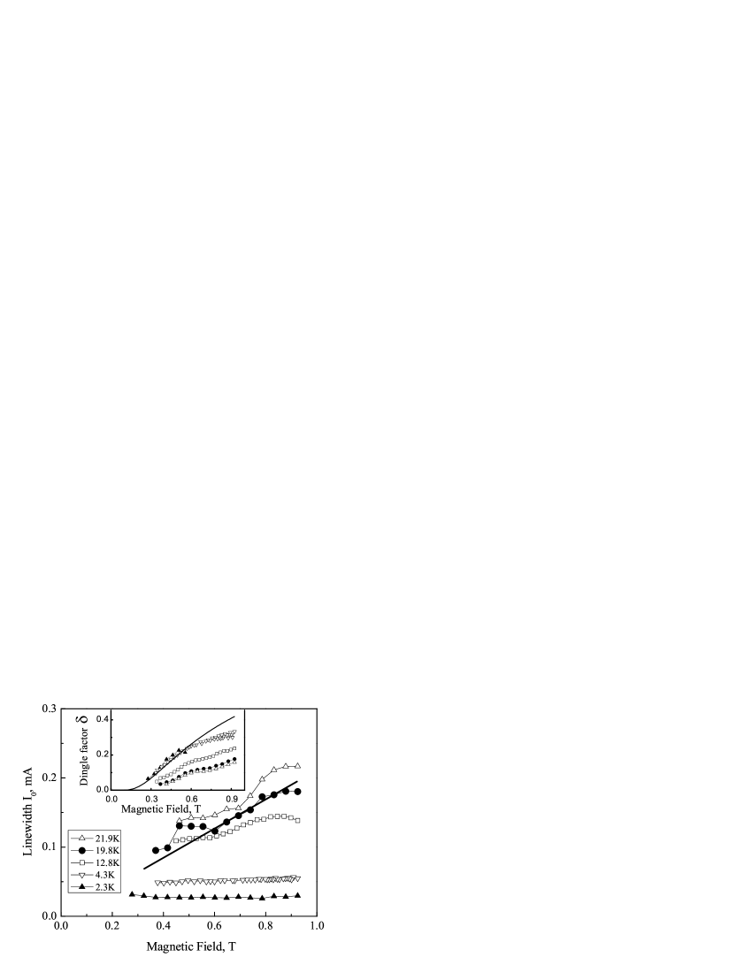
Figure 3: Dependence of the width of the peak $I_{0}$ on magnetic field at different temperatures, as labeled. The solid line represents the linear dependence expected from the theory in the high temperature limit (see Eq. 2). The inset shows the magnetic field dependence of the parameter $\delta$ obtained from the fit of the zero bias peak using Eq. 3. The solid line shows the theoretical dependence of the Dingle parameter $\delta$ on magnetic field, corresponding to a quantum scattering time $\tau_{q}$=1.5 (ps).

The dependence of the width of the peak ($I_{0}$) on magnetic field is presented in Fig. 3 at different temperatures. At high temperature the peak width varies considerably with magnetic field. The approximately linear increase of the scale $I_{0}$ with magnetic field agrees with the theory. The deviations from the linear dependence are beyond the scope of the theory. The oscillations may be related to magneto-phonon resonances observed in these systems at high temperature bykov2 . At low temperature, a regime that has not been considered by the theory, the width of the zero bias peak is found not to depend on magnetic field.

For several different temperatures, the insert to Fig. 3 shows the magnetic field dependence of the Dingle parameter, $\delta$, which is obtained from comparison of the magnitude of the zero bias peak with the theory (see Eq. 3). The parameter $\delta$ decreases with decreasing magnetic field, and disappears below H=0.2T. Using theoretical expression for the Dingle parameter dmitriev $\delta=exp(-\pi/\omega_{c}\tau_{q})$, we have plotted the parameter $\delta$ vs magnetic field using the quantum scattering time $\tau_{q}$ as a fitting parameter. This is shown in the insert by the solid line. The obtained quantum time $\tau_{q}=$1.5 (ps) is close to the quantum time extracted from the usual analysis of SdH oscillations at different temperature and/or magnetic field. A comparison between these two results is shown in the bottom insert to Fig. 4. Using this new method the time $\tau_{q}$ is found for temperatures up to 24K, where SdH oscillations are not detectable and previous methods fail to work. Thus the method extends considerably the temperature range, where the quantum scattering time can be studied.

Figure 4: Dependence of the width of the zero bias peak $I_{0}$ on temperature for sample N1 (open cirles) and sample N2 (open squares) at H=0.925T. The solid lines are the theory using Eqs. 2 and 3. The comparison gives an inelastic scattering time $\tau_{in}=10/T^{2}$($12/T^{2}$)(ns) for sample N1(N2). The top inset shows the transport time $\tau_{tr}$ vs temperature at zero magnetic field. The dependence of the quantum scattering time $\tau_{q}$ on temperature is shown in the bottom insert. Open squares correspond to $\tau_{q}$ determined from the amplidute of the SdH oscillations using Lifshits-Kosevich formulaeando . Filled squares are the $\tau_{q}$ determined by comparison of the amplidute of the zero bias peak with Eq. 3.

The temperature dependence of the width of the peak is shown in Fig. 4 heating . At low temperatures the width of the peak is found to be proportional to the temperature $T$. The linear temperature behavior of the $I_{0}$ indicates the quadratic temperature dependence of the inelastic scattering time: $\tau_{in}=\alpha/T^{2}$ (see eq.2), where $\alpha$ is a constant. This is in agreement with the theorydmitriev . At higher temperature a noticeable sublinear deviation is observed. This can also be captured by the theory if the temperature variations of the transport scattering time $\tau_{tr}$ is significant. The temperature dependence of $\tau_{tr}$ determined from the resistivity at zero magnetic field is shown in the top insert to the figure. The solid lines in the main figure are theoretical curves plotted in accordance with eq.2 and eq.3 in which the temperature variations of the $\tau_{tr}$ are taken into account and the constant $\alpha$ is the only fitting parameter. For the inelastic time we have found $\tau_{in}^{(1)}=10\times 10^{-9}/T^{2}$ (s) and $\tau_{in}^{(2)}=12\times 10^{-9}/T^{2}$ (s) for sample 1 and 2 . The corresponding theoretical estimations dmitriev of the inelastic time give $\tau_{in,t}^{(1)}=4.8\times 10^{-9}/T^{2}$ (s) and $\tau_{in,t}^{(2)}=3.2\times 10^{-9}/T^{2}$ (s). We consider this as satisfactory agreement, in light of several approximations used in the theory. The somewhat larger values of the inelastic time $\tau_{in}$ obtained in the experiment could also be due to additional electron screening of 2D electrons by X-electrons in AlAs/GaAs type-II superlattices fried . At high temperature $T>30$ K a considerable super-linear temperature dependence of the linewidth is found (not shown for sample N2). This phenomenon has been left for a future study.

In summary, a strong reduction of the longitudinal resitivity of 2D electrons in classically strong magnetic fields is observed in response to DC electric field. We have found that the effect is not related to Joule heating even at temperatures down to 2K, where strong quantum oscillations (SdH) are present that are highly sensitive to the temperature. At low temperature (2-10K), the scale of the electric fields at which the effect occurs is proportional to the temperature. Reasonable agreement is established with recent theory dmitriev that has predicted significant and nontrivial variations of the electron distribution function in response to a DC electric field. The comparison with the theory allowed us to find inelastic electron-electron scattering time $\tau_{in}$ and the quantum scattering time $\tau_{q}$ of the 2D electrons at high temperatures where previous methods, based on analysis of quantum oscillations, fail.

- (1) M.A. Zudov, R. R. Du, J. A. Simmons, and J. L. Reno, Phys. Rev. B 64,201311(R) (2001);
- (2) P.D. Ye, L. W. Engel, D.C. Tsui, J. A. Simmons, J. R. Wendt, G. A. Vawter, and J. L. Reno, Appl. Phys.Lett 79,2193 (2001).
- (3) R. G. Mani, V.Narayanamurti, K. von Klitzing, J. H. Smet, W. B. Jonson, and V. Umansky, Nature(London) 420, 646 (2002)
- (4) M.A. Zudov, R. R. Du, L. N. Pfeiffer, and K. W. West, Phys. Rev. Lett 90 046807 (2003).
- (5) S. I. Dorozhkin, JETP Lett. 77, 577 (2003).
- (6) R. L. Willett, L. N. Pfeiffer, and K. W. West, Phys. Rev. Lett 93 026804 (2004).
- (7) A. V. Andreev, I. L. Aleiner, and A. J. Millis, Phys.Rev. Lett. 91, 056803 (2003)
- (8) A. C. Durst, S. Sachdev, N. Read, and S. M. Girvin, Phys. Rev. Lett. 91, 086803 (2003)
- (9) P. W. Anderson and W. F. Brinkman, cond-mat/0302129
- (10) J. Shi and X. C. Xie, Phys. Rev. Lett. 91, 086801 (2003).
- (11) M. G. Vavilov and I. L. Aleiner Phys. Rev. B 69, 035303 (2004)
- (12) I. A. Dmitriev, M.G. Vavilov, I. L. Aleiner, A. D. Mirlin, and D. G. Polyakov, Phys. Rev. B 71, 115316 (2005).
- (13) S. I. Dorozhkin, J. H. Smet, V. Umansky and K. von Klitzing Phys. Rev. B 71, 201306(R) (2005).
- (14) C. L.Yang, J. Zhang, and R. R. Du, J. A. Simmons and J. L. Reno, Phys. Rev. Lett. 89, 076801 (2002)
- (15) A. A. Bykov, Jing-qiao Zhang, Sergey Vitkalov, A. K. Kalagin, and A. K. Bakarov Phys. Rev. B 72, 245307 (2005)
- (16) The actual (not differential) resistance is 12.7 Ohm at DC bias 0.08 mA and H=0.92T in Fig.2b. This is considerably below the baseline value: average between resistances at maximum and nearest minimum (26-28 ).
- (17) K. J. Friedland, R. Hey, H. Kostial, R. Klann, and K. Ploog, Phys.Rev.Lett. 77, 4616 (1996).
- (18) Although the theory is developed in high temperature limit, we have used the formula (2) and (3) to find width of the peak and it’s amplitude at all temperatures. Other fitting functions (procedures) do not change significantly the results presented in fig.3 and fig.4.
- (19) T. Ando, A. B. Fowler and F. Stern, Rev. Mod. Phys. 54, 437 (1982).
- (20) A. A. Bykov, A. K. Kalagin, and A. K. Bakarov JETP Lett.81, 523 (2005).
- (21) Using energy relaxation rate measured in GaAs/AlGaAs (see ”E. Chow et al Phys. Rev. Lett. 7, 1143 1996) we have estimated the electron temperature at DC biases relevant to the zero bias peak. Negligibly small electron overheating by the DC biases is found: at T=4.2K and at T=10K