Quantum criticality, lines of fixed points, and phase separation in doped two-dimensional quantum dimer models

Abstract

We study phase diagrams of a class of doped quantum dimer models on the square lattice with ground-state wave functions whose amplitudes have the form of the Gibbs weights of a classical doped dimer model. In this dimer model, parallel neighboring dimers have attractive interactions, whereas neighboring holes either do not interact or have a repulsive interaction. We investigate the behavior of this system via analytic methods and by Monte Carlo simulations. At zero doping, we confirm the existence of a Kosterlitz-Thouless transition from a quantum critical phase to a columnar phase. At low hole densities we find a dimer-hole liquid phase and a columnar phase, separated by a phase boundary which is a line of critical points with varying exponents. We demonstrate that this line ends at a multicritical point where the transition becomes first order and the system phase separates. The first-order transition coexistence curve is shown to become unstable with respect to more complex inhomogeneous phases in the presence of direct hole-hole interactions. We also use a variational approach to determine the spectrum of low-lying density fluctuations in the dimer-hole fluid phase.

I Introduction

The behavior of doped Mott insulators is a long-standing open and challenging problem in condensed-matter physics. Mott insulators are the parent states of all strongly correlated electronic systems and as such play a crucial role in our understanding of high-$T_{c}$ superconductors (HTSC) and many other systems. Their strongly correlated nature implies that their behavior cannot be understood in terms of weakly coupled models. Except for the very special case of one spatial dimension, the physics of doped Mott insulators is currently only understood at a qualitative level. The solution of this challenging problem remains one of the most important directions of research in condensed-matter physics.

Quantum dimer models (QDM)Rokhsar and Kivelson (1988) provide a simplified, and rather crude, description of the physics of a Mott insulator. They provide a correct description of the physics of Mott insulators in regimes in which the spin excitations have a large spin gap. QDMs were proposed originally within the context of the resonating-valence bond (RVB) mechanism of HTSC.Anderson (1987); Kivelson et al. (1987) These systems are of great interest as they can yield hints on the behavior of more realistic models of quantum frustration.

The main idea behind the formulation of QDMs is that, if the spin gap is large, the spin degrees of freedom become confined in tightly bound singlet states which, in the extreme limit of a very large spin gap, extend only over distance scales of the order of nearest-neighbor sites of the lattice. Thus, in this extreme regime, the Hilbert space can be approximately identified (up to some important caveatsRokhsar and Kivelson (1988)) with the coverings of the lattice by valence bonds or dimers.

Surprisingly, even at the level of the oversimplified picture offered by QDMs, the physics of doped Mott insulators remains poorly understood. In this paper we explore the phase diagrams, and the properties of their phases, of QDMs generalized to include interactions between dimers (or valence bonds), and between dimers and doped (charged) holes. Basic aspects of the physics of these models are reviewed in Ref. Fradkin, 1991 and references therein.

Undoped QDMs have been studied more extensively and by now they are relatively well understood.Read and Sachdev (1991); Sachdev and Read (1991); Moessner and Sondhi (2001); Moessner et al. (2002); Fradkin et al. (2003); Vishwanath et al. (2004); Ardonne et al. (2004) On bipartite lattices, their ground states show either long-range crystalline valence bond order of different sorts or are quantum critical,Rokhsar and Kivelson (1988); Fradkin (1991); Moessner et al. (2002) while on non-bipartite lattices their ground states are typically disordered and are topological fluids.Moessner and Sondhi (2001)

The more physically relevant doped QDMs, with a finite density of charge carriers (holes), are much less understood, although some properties are known.Fradkin and Kivelson (1990); Balents et al. (2005); Alet et al. (2005); Syljuasen (2005); Alet et al. (2006); Castelnovo et al. (2007); Poilblanc et al. (2006) In QDMs a spin-$\frac{1}{2}$ hole fractionalizes into a bosonic holon, an excitation that carries charge but no spin, and a spinon, a fermionic excitation that carries spin but no charge.Kivelson et al. (1987); Rokhsar and Kivelson (1988); Fradkin and Kivelson (1990); Fradkin (1991) Holons can be regarded as sites that do not belong to any dimer, whereas spinon pairs are broken dimers. This form of electron fractionalization is observable in the spectrum of these systems only in the topological disordered (spin-liquid) phases of the undoped QDM. Otherwise, as in the case of the valence bond crystalline states which exhibit long range dimer order, spinons and holons are confined and do not exist as independent excitations.Fradkin (1991)

In this paper, we consider several interacting QDMs on a square lattice at finite hole doping, and discuss their possible phases and phase transitions as a function of hole density and strength of the interactions. At any finite amount of doping the system will have a finite density of holes, which are hard core charged bosons in this description. To simplify the problem, in this work we do not consider the physical effects of the charge-neutral fermionic spinons which in principle should also be present. Thus, at this level of approximation, all spin-carrying excitations are effectively projected out. The remaining degrees of freedom are thus dimers (“spin-singlet valence bonds”) and charged hard-core bosonic holes. Already this simplified picture of a strongly correlated system is very non-trivial.

For a certain relation between its coupling constants, known as the Rokhsar-Kivelson (RK) condition,Rokhsar and Kivelson (1988) QDM Hamiltonians, both with and without holes, can be written as a sum of projection operators. These RK Hamiltonians are manifestly positive definite operators. For this choice of couplings, the ground-state wave function is a zero-energy state which is known exactly. This RK wave function is a local function of the degrees of freedom of the QDM, the local dimer and hole densities. The quantum-mechanical amplitudes of the RK wave functions turn out to have the same form as the Gibbs weights of a two-dimensional (2D) classical dimer problem with a finite density of holes. For the generalized doped QDMs that we consider, the norm of the exact ground-state wave function is equal to the partition function of a system of interacting classical dimers at finite hole density. This mapping to a 2D classical statistical mechanical system, for which there is a wealth of available results and methods, makes this class of problems solvable.Rokhsar and Kivelson (1988); Moessner and Sondhi (2001); Ardonne et al. (2004); Castelnovo et al. (2007)

In this work we will investigate the behavior of doped QDMs which satisfy the RK conditions by studying the correlations encoded in their ground state wave functions. The phase diagrams of these systems turn out to be quite rich. As we shall see, these simple models can describe many aspects of the physics of interest in strongly correlated systems, including a dimer-hole liquid phase (a Bose-Einstein condensate of holes), valence-bond crystalline states, phase separation, and more general inhomogeneous phases. The undoped version of this system was studied in detail in Ref. Alet et al., 2005, where a quantum phase transition was found that was argued to belong to the Kosterlitz-Thouless (KT) universality class, from a critical phase to a columnar state with long-range order. In this paper we confirm that this is indeed the case. At finite hole density, hitherto available results are limited to the form of the associated RK QDM HamiltonianCastelnovo et al. (2007); Poilblanc et al. (2006) and numerical results for small systems.

In this work we employ analytic methodsKadanoff (1977); Ginsparg (1989); Boyanovsky (1989); Lecheminant et al. (2002) combined with advanced classical Monte Carlo (MC) simulationsKrauth and Moessner (2003); Liu and Luijten (2004) to probe the correlations in the doped RK wave functions, investigate the phase diagram and its phase transitions. The methods used here can be readily generalized to the case of non-bipartite lattices, for which a number of important results have been published.Moessner and Sondhi (2001); Fendley et al. (2002); Trousselet et al. (2007) In Section II, we describe the construction of two generalized quantum dimer RK Hamiltonians that we used in our study. A similar but independent construction has been presented by Castelnovo and coworkersCastelnovo et al. (2007) and by Poilblanc and coworkersPoilblanc et al. (2006). The RK wave functions of these generalizations of the quantum dimer model have either a fixed number of holes or a variable number of holes and a fixed hole fugacity. The ground-state wave functions of both models at their associated RK points correspond to a canonical dimer-monomer system in the canonical and grand-canonical ensembles respectively. Near the end of the paper, in Section VI, we introduce a third Hamiltonian, with an associated RK wave function, to study the effects of hole interactions which compete with phase separation at the first-order transitions that we find for both models.

In Sections III and IV we study the correlations and the phase diagram for the ground states encoded in these wave functions by means of an analysis of the equivalent classical statistical system of dimers and holes for the RK Hamiltonians of Section II. In Section III we summarize the results of a mean-field theory for both non-interacting and interacting classical dimer models at finite doping. The details of the mean-field theory are presented in Appendix A, where we compute the hole-hole correlation function and derive a qualitative phase diagram as a function of hole density and dimer interaction parameters. The main result of this simple mean-field theory is that the phase diagram at finite hole density contains two phases, a dimer-hole fluid and a columnar dimer solid. The columnar-liquid transition is continuous at weak coupling and turns first order at a tricritical point. Naturally, the critical and tricritical behavior are not correctly described by the mean-field theory, although the general topology of the phase diagram is correct and, remarkably, even the location of the tricritical point is consistent with what we find in the MC simulations of Section V.

In Section IV we present a detailed analytic theory of the critical behavior of interacting classical dimers. Sections IV.1 and IV.2 focus on the field-theoretic Coulomb-gas approach for this model at zero and finite doping, respectively. We show that, up to a critical value of a parameter, the undoped RK wave function describes a critical system with continuously varying critical exponents, with a phase transition (belonging to the 2D KT universality class) to a state with long-range columnar order. At finite hole doping we find a hole-dimer liquid phase (with short-range correlations) and a stable phase with long-range columnar order. At low hole densities the phase boundary is a line of fixed points with varying exponents ending at a KT-type multicritical point where the transition becomes first order. We present a field-theoretical treatment of this tricritical point and a theory of the evolution of the behavior of the columnar and orientational order parameters and of their susceptibilities along the phase boundary. Past the tricritical point the system is found to exhibit a strong tendency to phase separation, which we verify in our numerical simulations (Section V). In Section VI we consider the effects of direct hole-hole interactions near the first-order phase boundary, and discuss one of the many inhomogeneous phases which arise in this regime instead of phase separation.

In Section V we confirm our analytic predictions via extensive classical MC simulations of the generalized RK wave functions. For the study of the line of critical points at low doping we employ the canonical generalized geometric cluster algorithm (GGCA), whereas the first-order transition is studied via grand-canonical Metropolis-type simulations. The GGCA algorithm enables us to study relatively large systems, up to $400\times 400$, for a range of dopings, $0\leq x\leq 0.06$, and to investigate the finite-size scaling behavior. The accessible range of system sizes should be compared to what can be reached for full quantum models, away from the RK condition, where available methods, such as exact diagonalization and Green function Monte Carlo, allow the study of only very small systems with few holes.Syljuasen (2005); Poilblanc et al. (2006)

In the undoped case we confirm the existence of a Kosterlitz-Thouless transition from a line of critical points to an ordered columnar state, as found in the work of Alet and coworkers.Alet et al. (2005, 2006) We study the scaling behavior of the columnar and orientational order parameters and of their susceptibilities. We also use a mapping of the orientational order parameter of the interacting classical dimer model to the staggered polarization operator obtained by Baxter for the six-vertex modelBaxter (1973) to fit our MC data and find an accurate estimate of the KT transition coupling in the undoped case.

At low doping, we study the transition from the dimer-hole fluid phase to the columnar state. We confirm that the scaling dimension of the columnar order parameter operator is equal to $1/8$, as predicted by our analytic results of Section IV.2. We also present a typical set of data that demonstrates how the scaling dimension of the orientational order parameter varies, again in agreement with the analytic results of Section IV.2, and use these results to locate numerically the phase boundary. We then turn to the behavior at larger doping and stronger couplings where the transition becomes first order. We study this regime using grand-canonical Metropolis Monte Carlo simulations. We confirm the first-order nature of the phase transition by means of a careful analysis of the finite-size scaling behavior of the order parameters across the phase boundary and of their susceptibilities. We use these results to locate the phase boundary in the first-order regime as well. In Section VI, we use MC simulations to study the effects of a direct hole-hole repulsion which suppresses the effects of phase separation, leading instead to a complex phase diagram of inhomogeneous phases, of which we only study its most commensurate case.

In Section VII, we study the elementary quantum excitations of the doped QDMs satisfying the RK condition using the single-mode approximation. We only present the main results and have relegated the details to Appendix B. We find that in the dimer-hole liquid phase, hole and dimer density fluctuations have quadratic dispersions $E(k)\sim k^{2}$. Thus this phase should be characterized as a Bose-Einstein condensate of bosonic charged particles (holes), but not really a superfluid, for reasons similar to those of Rokhsar and Kivelson.Rokhsar and Kivelson (1988) We summarize our overall conclusions in Section VIII.

While this manuscript was being completed (and refereed) a number of independent studies of aspects of this problem have been published.Castelnovo et al. (2007); Poilblanc et al. (2006); Alet et al. (2006) Our results agree with those in these references wherever they overlap, as noted throughout this paper.

II Quantum Hamiltonians for Interacting Dimers at Finite Hole Density

The Hamiltonian of the quantum dimer model (QDM) can be written in the Rokhsar-Kivelson (RK) formRokhsar and Kivelson (1988) as the sum of a set of mutually non-commuting projection operators $Q_{p}$,

$$H=\sum_{\{p\}}Q_{p}\;,$$ (1)

where $\{p\}$ denotes the set of all plaquettes of the square lattice. Each projection operator $Q_{p}$ acts on the states of the dimers and holes of a plaquette $p$ (or set of plaquettes surrounding $p$). In the simplest caseRokhsar and Kivelson (1988) each $Q_{p}$ acts only on the states labeled by the dimer occupation numbers of the links of the plaquette $p$. In this case, the ground state is described by the short-range RVB wave functionKivelson et al. (1987)

$$|\textrm{RVB}\rangle=\sum_{\{\mathcal{C}\}}|\mathcal{C}\rangle\;,$$ (2)

where $\{\mathcal{C}\}$ is the set of (fully packed) dimer coverings of the 2D square lattice, and $\{|\mathcal{C}\rangle\}$ is a complete set of orthonormal states. If one regards the dimers as spin singlet states (with the spins residing on the lattice sites) each configuration represents a set of spin singlets or valence-bonds.Anderson (1987); Kivelson et al. (1987) The dimer representation ignores the over-completeness of the valence bond singlet states.Rokhsar and Kivelson (1988) This problem can be made parametrically small using a number of schemes, including large $N$ approximationsRead and Sachdev (1989) and decorated generalizations of the spin-$1/2$ Hamiltonians.Raman et al. (2005)

It is possible and straightforward to generalize the QDM construction so as to include other types of interactions and coverings. In Ref. Ardonne et al., 2004 it was shown how to extend this structure to smoothly interpolate between the square and the triangular lattices. It was also shown there that the same ideas can be used to construct a quantum generalization of the two-dimensional classical Baxter (or eight-vertex) model. In all of these cases, the RK form of this generalized quantum dimer model has an exact ground-state wave function whose amplitudes are equal to the statistical (Gibbs) weights of an associated two-dimensional classical statistical mechanical system on the same lattice. Thus, if the classical problem happens to be a classical critical system, the associated wave function now describes a 2D problem at a quantum critical point. In Ref. Ardonne et al., 2004 such quantum critical points were dubbed “conformal quantum critical points” since the long-distance structure of their ground-state wave functions exhibits 2D conformal invariance. Here we are interested in a different generalization of the QDM in which we consider dimer coverings (although not necessarily fully packed) of the square lattice. We will also consider 2D Hamiltonians whose wave functions correspond to classical interacting 2D dimer problems with local weights. Similar but independent constructions have also been proposed.Castelnovo et al. (2005, 2007); Poilblanc et al. (2006)

Trying to be as physical and local as possible, we keep the quantum-resonance terms as simple as before (single plaquette moves), but the potential terms (which again have a central plaquetteKivelson et al. (1987)) now have fine-tuned couplings that depend on the nearby plaquettes. Explicitly, we have (cf. Fig. 1):

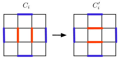
Figure 1: (color online) Illustration to clarify the construction of the Hamiltonian (LABEL:Ham). The central dimer pair is present in all configurations $C_{i}$ and $C_{i}^{\prime}$, whereas the four surrounding dimers may or may not be present. The index $i$ enumerates the $2^{4}$ possible arrangements of the surrounding dimers. The configuration $C^{\prime}$ differs from the corresponding $C$ by a single flip resonance of the central dimer pair.

$$H_{d} = t\sum_{i}\Bigg{[}-\Big{|}C_{i}\Big{>}\Big{<}C_{i}^{\prime}\Big{|}-\Big{|}C_{i}^{\prime}\Big{>}\Big{<}C_{i}\Big{|}$$

$$+ w^{R_{C_{i}^{\prime}}-R_{C_{i}}}\Big{|}C_{i}\Big{>}\Big{<}C_{i}\Big{|}+w^{R_{C_{i}}-R_{C_{i}^{\prime}}}\Big{|}C_{i}^{\prime}\Big{>}\Big{<}C_{i}^{\prime}\Big{|}\Bigg{]}\;,$$

where $R_{C_{i}}$ and $R_{C_{i}^{\prime}}$ denote the number of pairs of present dimers formed in configurations $C_{i}$ and $C_{i}^{\prime}$ respectively.

The Hamiltonian of Eq. (LABEL:Ham) is designed in such a way that it annihilates any superposition of dimer-configuration states which have amplitudes that are of the form $w^{N_{p}}$, where $w$ is the parameter appearing in the Hamiltonian and $N_{p}$ is the number of pairs of neighboring dimers in the configuration.Ardonne et al. (2004) In this sense, the Hamiltonian is a sum of projection operators and consequently there is a unique ground state for each topological sector which must be composed of the superposition of these specially weighted configurations. The ground-state wave function, $|G\rangle$, the state annihilated by all the projection operators, for this system is:

$$|G\rangle=\frac{1}{\sqrt{Z(w^{2})}}\sum_{\{\mathcal{C}\}}w^{\displaystyle{N_{p}[\mathcal{C}]}}|\mathcal{C}\rangle\;,$$ (4)

where $Z(w^{2})$, the normalization of this state,

$$Z(w^{2})=\sum_{\{\mathcal{C}\}}w^{\displaystyle{2N_{p}[\mathcal{C}]}}$$ (5)

has the form the partition function of classically interacting dimers with a coupling $u=-2\ln w$ between parallel neighboring dimers. In the following, we will assume an attractive coupling, $u<0$ or $w>1$. The case $u>0$ was studied for the fully-packed case in Ref. Castelnovo et al., 2007.

There are two different ways in which we can add doping to our system, while still being able to determine the ground state. If we add the following fine-tuned hole-related terms to the initial Hamiltonian (LABEL:Ham)

$$H^{\rm hole}_{\rm canonical}=-t_{\rm hole}\sum_{<ijk>}\Bigg{\{}\Bigg{[}\Big{|}\raisebox{-2.15277pt}{\includegraphics{Ham22.eps}}\Big{>}\Big{<}\raisebox{-2.15277pt}{\includegraphics{Ham23.eps}}\Big{|}+\mathit{h.c.}\Bigg{]}$$

$$-\Big{|}\raisebox{-2.15277pt}{\includegraphics{Ham22.eps}}\Big{>}\Big{<}\raisebox{-2.15277pt}{\includegraphics{Ham22.eps}}\Big{|}-\Big{|}\raisebox{-2.15277pt}{\includegraphics{Ham23.eps}}\Big{>}\Big{<}\raisebox{-2.15277pt}{\includegraphics{Ham23.eps}}\Big{|}\Bigg{\}}$$ (6)

then the resulting ground state becomes

$$|G_{N_{h}}\rangle=\frac{1}{\sqrt{Z(w^{2})}}\sum_{\{\mathcal{C}_{N_{h}}\}}w^{\displaystyle{N_{p}[\mathcal{C}_{N_{h}}]}}|\mathcal{C}_{N_{h}}\rangle\;,$$ (7)

where the number of holes $N_{h}$ is now fixed at a specified value. The norm of this wave-function, $Z(w^{2})$, is the canonical partition function for the set of dimer coverings with a fixed number of holes.

On the other hand, if we add the following terms, which do not conserve the number of holes in the system, to the Hamiltonian (LABEL:Ham)

$$H^{\rm hole}_{\rm{grand-canonical}}=-\tilde{t}_{\rm hole}\sum_{links}\Bigg{\{}\Bigg{[}\Big{|}\raisebox{-2.15277pt}{\includegraphics[scale={0.6}]{Ham20.eps}}\Big{>}\Big{<}\raisebox{-2.15277pt}{\includegraphics[scale={0.6}]{Ham21.eps}}\Big{|}+h.c.\Bigg{]}$$

$$-z^{2}\Big{|}\raisebox{-2.15277pt}{\includegraphics[scale={0.6}]{Ham20.eps}}\Big{>}\Big{<}\raisebox{-2.15277pt}{\includegraphics[scale={0.6}]{Ham20.eps}}\Big{|}-z^{-2}\Big{|}\raisebox{-2.15277pt}{\includegraphics[scale={0.6}]{Ham21.eps}}\Big{>}\Big{<}\raisebox{-2.15277pt}{\includegraphics[scale={0.6}]{Ham21.eps}}\Big{|}\Bigg{\}}$$

(8)

then the ground state of the system becomes

$$|G\rangle=\frac{1}{\sqrt{Z(w^{2},z^{2})}}\sum_{\{\mathcal{C}\}}w^{\displaystyle{N_{p}[\mathcal{C}]}}z^{\displaystyle{N_{h}[\mathcal{C}]}}|\mathcal{C}\rangle\;,$$ (9)

with

$$Z(w^{2},z^{2})=\sum_{\{\mathcal{C}\}}w^{2N_{p}[\mathcal{C}]}z^{2N_{h}[\mathcal{C}]}\;.$$ (10)

Equation (8) includes a natural, short-range repulsion between neighboring holes and an off-diagonal term which represents creation-annihilation of dimers. Furthermore, there is a dimer fugacity term, as in every perturbative derivation of a quantum dimer model.Rokhsar and Kivelson (1988) We note that Eq. (10) has the same form as a grand partition function for dimer coverings of the square lattice. This partition function now depends not only on the interaction $u$ defined below Eq. (5), but also on the hole chemical potential $\mu/|u|=2\ln z$.

Since the canonical and grand-canonical ensembles become equivalent in the thermodynamic limit, the two ground-state wave functions (7) and (9) must correspond to the same ground-state physics. Furthermore, it is clear that for $w=1$ the models are located at the usual RK point of the quantum dimer model on the square lattice. For a system with periodic boundary conditions, each configuration $\mathcal{C}$ contains only an even number of holes, with half of the holes on either sublattice.

We remark that the fact that the exact ground-state wave function is a sum (as opposed to a product) of the ground states of sectors labeled by the number of holes on the lattice, is due to the resonance term that we have used to represent the motion of holes. In particular, we have assumed that a dimer can break into two holes which themselves repel each other. In the limit of very strong hole-hole repulsions, in strong-coupling perturbation theory, it is straightforward to recover a fixed-hole density sector with a single-hole resonance move involving three sites in any direction; the coupling strength in Eq. (6) then becomes $t_{\rm hole}\sim z^{4}\tilde{t}_{\rm hole}$, and thus, in the limit $z\rightarrow 0$, it reduces to an effective hopping amplitude for the holes.

III Mean-Field Results

To examine the physics described by the ground-state wave functions obtained in the previous section we start with a discussion of a mean-field theory of the phase diagram. We use the standard approach of regarding the probability densities, obtained by squaring the wave function, as the Gibbs weights of a classical two-dimensional system and focus on the interacting dimer model on the square lattice at finite hole density. Although mean-field theory is insufficient to describe two-dimensional critical systems, it is a useful tool to obtain qualitative features of the phase diagram as well as the behavior deep in the phases, away from criticality.

The details of this theory are presented in Appendix A. We begin by constructing a Grassmann representation of the partition function for an interacting dimer model using the standard methods introduced by Samuel.Samuel (1980a, b) The resulting theory involves Grassmann (anti-commuting) variables residing on the sites of the square lattice. The action of the Grassmann integral is non-trivial and is parametrized by the hole fugacity $z$ and a coupling between dimers $V=z^{2}(e^{u}-1)$, where $u=-2\ln w$.

Since the action of the resulting Grassmann path integral is not quadratic in the Grassmann variables, it cannot be reduced to the computation of a determinant. Thus, we use a standard mean-field approach which, in this case, involves the introduction of two Hubbard-Stratonovich (bosonic) fields $\phi_{i}$ and $\chi_{ij}$, defined on the sites and links of the square lattice respectively. Upon integrating out the Grassmann variables one obtains an effective theory for the fields $\phi_{i}$ and $\chi_{ij}$ which, as usual, is solved within a saddle-point expansion. The dimer $m_{0}$ and hole $n$ densities, as well as the columnar order parameter $m$, can be expressed straightforwardly in terms of the fields $\phi_{i}$ and $\chi_{ij}$. From this effective theory one can compute an effective potential $\Gamma$ and the configurations of the observables of interest, $n$, $m_{0}$ and $m$, as functions of $z$ and $V$, and determine the phase diagram.

As a function of hole density (or hole fugacity) and $u$, we find that the phase diagram has two phases (shown qualitatively in Fig. 2), namely a dimer-hole liquid phase and a hole-poor phase with long-range columnar order. The nature of the transitions between these phases is incorrectly described by the mean-field theory, particularly at zero doping and near the tricritical point. The correct behavior is the subject of a detailed analysis in the subsequent sections. Nevertheless, the mean-field phase diagram correctly predicts that at low hole densities and moderate values of $u$ the transition between the dimer-hole liquid and the columnar solid phase is continuous, that for large $u$ the transition is first order, and that there is a tricritical point at

$$u_{tr}\simeq 2.733,\qquad z_{tr}\simeq 0.075\;.$$ (11)

Remarkably, the Monte Carlo simulations presented in Section V yield a tricritical point at a location quite consistent with these values.

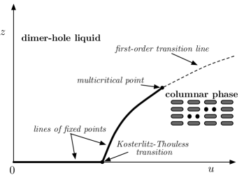
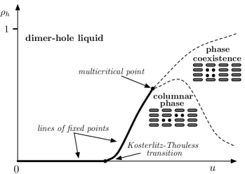
Figure 2: Qualitative phase diagrams for the interacting doped dimer model. a) Phase diagram as a function of the fugacity $z$ for the holes and $u=-\ln w$, the dimer interaction coupling constant. The line of continuously varying exponents for low fugacity evolves to a line of first-order transitions. b) Phase diagram in terms of the hole density $\rho_{h}$ and the coupling constant $u$. Here the line of first-order transitions opens up into a two-phase coexistence region.

Another correct prediction of the mean-field theory is the behavior of the connected hole density correlation function deep in the dimer-hole liquid phase. This prediction, also discussed in detail in Appendix A, fits surprisingly well the Monte Carlo simulations of Krauth and Moessner,Krauth and Moessner (2003) performed for a system of classical non-interacting ($u=0$) dimers at finite hole density. The mean-field result is consistent with the simulations for a quite broad region of densities even quite close to the fully packed limit $z\to 0$ where, naturally, a wrong correlation length exponent is predicted.

IV Phase Diagram and Correlations for Interacting Dimers and Holes

We now turn to a more precise analysis of the phase transitions of the interacting classical dimer models as a function of hole density on interaction parameter $u$. Here we take advantage of a wealth of information and methods from two-dimensional systems, exact solutions and conformal field theory, to analyse the behavior in detail and extract conclusions that will be quite useful for the analysis of the wave functions. We begin with a discussion of the undoped case, and then discuss the physics at finite hole density.

IV.1 Interacting Dimers at Zero Hole Density

It is a well known fact that both classical and quantum two-dimensional dimer models can be represented in terms of height models. For the classical case, this mapping is well knownBlöte and Hilhorst (1982); Blöte and Nightingale (1982); Henley (1997); Ardonne et al. (2004). The mapping for the quantum case has also been discussed extensivelyFradkin and Kivelson (1990); Levitov (1990); Zheng and Sachdev (1989); Fradkin (1991); Ardonne et al. (2004); Fradkin et al. (2003). In both cases the mapping relates each dimer configuration to a configuration of a set of integer-valued (height) variables, $h(\vec{r})$, which reside on the sites of the dual lattice, a square lattice in the case of interest here. Thus, this mapping amounts to a duality transformation.

An alternative picture follows from realizing that dimer configurations can be mapped onto the degenerate ground-state configurations of fully frustrated Ising modelsBlöte and Hilhorst (1982); Moessner and Sondhi (2003a). In our case, the corresponding spin model is the fully frustrated Ising model on the square lattice (FFSI) at zero temperature. In the Ising model picture, each dimer is dual to an unsatisfied bond of the fully frustrated Ising model and classical dimer interactions correspond to second neighbor interactions in the square lattice FFSIFradkin and Forgacs (1981). It is easy to see that holes correspond to unfrustrated plaquettes in the FFSI. In this work we use primarily the language of the height representation.

To map the square-lattice classical dimer model onto a height model, we follow the prescription given in Ref. Ardonne et al., 2004. One first assigns a height variable to each plaquette. In going around a vertex on the even sub-lattice clockwise, the height changes by $+3$ if a dimer is present on the link between the plaquettes, and by $-1$ if no dimer is present on that link. On the odd sub-lattice, the heights change by $-3$ and $+1$ respectively. The dimer constraint, that one lattice site belongs to one and only one dimer, implies (for the square lattice) that, for the fully packed case, there are four possible configurations of dimers for each lattice site. In the dual height model this is reproduced by the period four property $h\equiv h+4$ of the allowed height configurations. It is easy to see that for the allowed configuration the average values that the height variables can take at a given site of the direct lattice (a vertex) are $\pm 3/2,\pm 1/2$. On the other hand, a uniform shift of all the heights by one unit, $h\to h+1$, leads to an equivalent state. This mapping works strictly speaking only for the fully packed case. Holes are sites that don’t belong to any dimer and thus represent violations of the full packing rule. They play the role of topological defects (“vortices”) in the (dual) height representation.

The exact solution of the non-interacting fully packed dimer model on the square (and other) lattice has been known for a long timeFisher and Stephenson (1963). In particular the long-distance behavior of the dimer density correlation functions and the hole density correlation functions are known explicitlyFisher and Stephenson (1963); Youngblood et al. (1980). These correlation functions obey power law behaviors and show that this is a critical system. Here we will use the standard approach to map the exact long distance behavior of two-dimensional critical systems to the behavior of the simplest critical system, the Gaussian or free boson modelKadanoff (1977). This approach is consistent for the free dimer model on an even lattice with periodic boundary conditions since its central charge (or conformal anomaly) is also $c=1$.

We will use as reference states (“ideal states” in the terminology of Kondev and HenleyKondev and Henley (1996)) the four columnar states of the dimer coverings, which have the largest number of flippable plaquettes, and use them to define an effective field theory for this problemFradkin et al. (2003). We will assign a uniform value to the coarse-grained height field $h=0,1,2,3$ to each reference (columnar) state. Let $n_{x}(\vec{r})$ and $n_{y}(\vec{y})$ represent the coarse grained dimer densities of the horizontal link with endpoints at the pairs of lattice sites $\vec{r}$ and $\vec{r}+\vec{e}_{x}$, and vertical links with endpoints $\vec{r}$ and $\vec{r}+\vec{e}_{y}$ respectively. Here $\vec{e}_{x}$ and $\vec{e}_{y}$ are two lattice unit vectors along the $x$ and $y$ directions respectively, with a lattice spacing of $1$.

We can now define the columnar local order parameter as the two component vector

$$\mathcal{O}_{x}(x,y) = n_{x}(x,y)-n_{x}(x+1,y)$$

$$\mathcal{O}_{y}(x,y) = n_{y}(x,y)-n_{y}(x,y+1)$$ (12)

which clearly correspond to the $(\pi,0)$ and $(0,\pi)$ Fourier components of the dimer densities. This two-component order parameter takes four distinct values for each one of the columnar states, and changes sign under shifts by one lattice spacing in either direction. It also transforms as a vector under $90^{\circ}$ rotations. Thus it is the order parameter for columnar order.

IV.1.1 Effective Field Theory: the non-interacting case

The fluctuations of the free field $h(\vec{r})$ are described by a continuum Gaussian (free boson) model. We will find it simpler to work with the rescaled height field $\phi=\frac{\pi}{2}h$. For this field the periodicity condition $h\to h+4$ becomes $\phi\to\phi+2\pi$. (For the rescaled field the ideal states are $\phi=0,\pi/2,\pi,3\pi/2$.) Thus, the allowed operators are $2\pi$ periodic functions of $\phi$, and are either derivatives of $\phi$, or the exponential (or charge) operators $\exp(\pm i\phi)$, $\exp(\pm 2i\phi)$, $\exp(3i\phi)$ and $\exp(\pm 4i\phi)$, which are $2\pi$ periodic functions of $\phi$.

The action $S$ for the rescaled field is

$$S=\int d^{2}x\frac{K}{2}\left(\nabla\phi\right)^{2}$$ (13)

For the free dimer model the stiffness is $K=\frac{1}{4\pi}$ (see below).

By matching the exact correlation functions of the free dimer model on the square lattice one readily finds the following operator identification of the coarse-grained dimer densities in terms of free field operatorsFradkin et al. (2003)

$$n_{x}-\frac{1}{4} = \frac{1}{2\pi}(-1)^{x+y}\partial_{y}\phi+\frac{1}{2}[(-1)^{x}e^{\displaystyle{i\phi}}+{\rm c.c.}]$$ (14)

$$n_{y}-\frac{1}{4} = \frac{1}{2\pi}(-1)^{x+y+1}\partial_{x}\phi+\frac{1}{2}[(-1)^{y}i\;e^{\displaystyle{i\phi}}+{\rm c.c.}]$$

In Ref. Fradkin et al., 2003 it was shown that this is an operator identity for the free dimer model on the square lattice in the sense the the asymptotic long-distance behavior of the dimer density correlation functions computed with this Gaussian model are the same as the exact long distance correlation functions for the free dimer problem on the square latticeFisher and Stephenson (1963); Youngblood et al. (1980) provided the stiffness $K=\frac{1}{4\pi}$. Notice that, with this identification, when the field $\phi$ takes each of the values $0,\pi/2,\pi,3\pi/2$ (the “ideal states”) the density operators take four distinct values which reflect the broken symmetries of the four columnar states.

From the operator identification of Eq. (LABEL:densities) the columnar order parameter is, up to a normalization constant,

$$\mathcal{O}_{x}=\cos\phi,\qquad\mathcal{O}_{y}=\sin\phi$$ (16)

Due to the effects of dimer-dimer interactions the form of this effective action is

$$S=\int d^{2}x\;\frac{K}{2}\left(\nabla\phi\right)^{2}+\textrm{perturbations}$$ (17)

The effect of the interactions is a finite renormalization of the stiffness $K$ away from its free dimer value, $K=\frac{1}{4\pi}$.

We saw above that, due to the dimer constraints, the allowed charge operators are $O_{n}(\vec{r})=\exp(in\phi(\vec{r}))$. We also saw that the columnar order parameter is proportional to the operator $\frac{1}{2}(O_{1}(\vec{r})+O_{-1})(\vec{r})=\cos\phi(\vec{r})$, and carries the unit of charge $n=1$. One can also define vortex or magnetic operatorsKadanoff (1977), and example of which is the hole. A vortex operator causes the field $\phi$ to wind by $2\pi m$, where $m$ is the vorticity (or magnetic charge). One can similarly define a general composite operator $O_{n,m}(\vec{r})$ with $n$ units of (electric) charge and $m$ units of vorticity (or magnetic charge). Its scaling dimensions, $\Delta(n,m)$ areKadanoff (1977)

$$\Delta_{n,m}(K)=\frac{n^{2}}{4\pi K}+\pi Km^{2}$$ (18)

We can now use these results to identify a few operators of interest and give their scaling dimensions. These results are summarized in Table 1

1. The columnar order parameter is the elementary charge operator $O_{\pm 1,0}$ and has no vorticity. On the (columnar) ideal states $0$, $\pi/2$, $\pi$, and $3\pi/2$ this operator takes the values $1$ ,$i$ ,$-1$, and $-i$ respectively. Its scaling dimension is $\Delta_{1,0}(K)=\frac{1}{4\pi K}$. At the free dimer point, $K=\frac{1}{4\pi}$, its scaling dimension is $\Delta_{1,0}(\frac{1}{4\pi})=1$. This is consistent with the exact resultsFisher and Stephenson (1963); Youngblood et al. (1980) that the density correlation function falls off as $1/r^{2}$. The operator identification of Eq. (LABEL:densities) is based on these factsFradkin et al. (2003).

2. The operator $O_{\pm 2,0}=\exp(\pm 2i\phi)$ takes the values $1$, $-1$, $1$ and $-1$ on each of the ideal columnar states. It is clearly the order parameter for symmetry breaking by $90^{\circ}$ rotations: it is the order parameter for orientational symmetry.

3. The operator with the highest allowed electric charge is $O_{\pm 4,0}=\exp(\pm 4i\phi)$. Its scaling dimension is $\Delta_{4,0}(K)=\frac{4}{\pi K}$. At the free dimer point it has dimension $\Delta_{4,0}(\frac{1}{4\pi})=16$, and it is a strongly irrelevant operator. This operator arises naturally due to the fact that the microscopic heights $h$ take integer values, and hence height configurations which differ by an uniform integer shift are physically equivalent. This operator does not break any physical symmetry of the dimer model.

4. The hole operator is represented by the fundamental vortex operator $O_{0,\pm 1}$. A vortex with unit positive magnetic charge corresponds to a hole on one sublattice, and a vortex with unit negative magnetic charge to a hole on the other sublattice. The scaling dimension of the vortex (hole) operator is $\Delta_{0,1}(K)=\pi K$. At the free dimer value, the scaling dimension of the hole operator is $\Delta_{0,1}(\frac{1}{4\pi})=\frac{1}{4}$, which is consistent with the exact result that the hole-hole correlation function decays $1/\sqrt{r}$ at large distancesFisher and Stephenson (1963).

5. The operator which describes a pair of holes on nearby sites of the same sublattice is represented by the operators $O_{0,\pm 2}$ which carry two units of magnetic charge (vorticity). This operator creates (or destroys) a diagonal dimer connecting nearby points on the same sublattice.Read and Sachdev (1991) In the $2+1$-dimensional quantum dimer model, this operator is useful to describe the possible pairing of holes. This operator has dimension $\Delta_{0,2}(K)=4\pi K$. Its scaling dimension at the free dimer point is $\Delta_{0,2}(\frac{1}{4\pi})=1$, and is relevant for $K<\frac{1}{2\pi}$. As noted in Refs. Fendley et al., 2002 and Ardonne et al., 2004, this operator maps the square lattice into a deformed triangular lattice. The irrelevancy of this operator for $K>\frac{1}{2\pi}$ implies that this line of fixed points also exists for a deformed triangular lattice, as discussed recently in Ref. Trousselet et al., 2007.

6. The free dimer problem is a free fermion system, which can be solved by Pfaffian methods.Fisher and Stephenson (1963); Samuel (1980a); Fendley et al. (2002) This is actually a theory with two free real (Majorana) fermions or, equivalently, one free complex (Dirac) fermion, at its (massless) fixed point, whose central charge is also $c=1$. The appropriate fermion operator is a composite operator of the order and disorder operatorsKadanoff (1977); Kadanoff and Ceva (1971) which, in this case, is $O_{\frac{1}{2},1}$. At the free dimer point the fermion operator has scaling dimension $\Delta_{\frac{1}{2},1}(\frac{1}{4\pi})=\frac{1}{2}$ and (conformal) spin $nm=\frac{1}{2}$ (as it should for a free fermion). At particular values of $K$ it is also possible to define parafermion operatorsFradkin and Kadanoff (1980); Zamolodchikov and Fateev (1985) operators which obey fractional statistics. For instance, at the KT point, $K=\frac{2}{\pi}$ (see below), the operator $O_{1,\frac{1}{4}}$ has dimension $\frac{1}{4}$ and spin $\frac{1}{4}$, and it is a semion. In fact, and not surprisingly, a fermionic approachFendley et al. (2002) can be used to map this critical line onto an Euclidean version of the Luttinger-Thirring model. The coarse-grained height model description we sue here corresponds to the bosonization approach of the fermionic version of this problem.

	${\rm columnar}$	${\rm rotational}$		${\rm hole}$	${\rm hole\;pair}$
	$O_{1,0}$	$O_{2,0}$	$O_{4,0}$	$O_{0,1}$	$O_{0,2}$
$K=\frac{1}{4\pi}$	$1$	$4$	$16$	$\frac{1}{4}$	$1$
$K=\frac{2}{\pi}$	$\frac{1}{8}$	$\frac{1}{2}$	$2$	$2$	$8$

Table 1: Scaling dimensions of the order parameters (charge) and hole (vortex) operators at the free dimer point, $K=\frac{1}{4\pi}$, and at the KT point, $K=\frac{2}{\pi}$.

IV.1.2 Effective Field Theory: interactions and phase transition

We now turn to the effects of dimer-dimer interactions. We recall that we are considering only interactions of a pair of dimers in a plaquette. The interaction energy is

$$H_{\rm int}=-u\sum_{\vec{r}}\Big{[}n_{x}(\vec{r})n_{x}(\vec{r}+\vec{e}_{y})+n_{y}(\vec{r})n_{x}(\vec{r}+\vec{e}_{x})\Big{]}$$ (19)

We wish to find the corresponding operator in terms of the coarse grained (rescaled) height field $\phi$. This can be done by using the operator product expansion (OPE) of the coarse-grained form of the dimer density operators, Eq. (LABEL:densities), in terms of the field $\phi$. We will also need the standard OPE of the (normal ordered) charge operatorsWitten (1978); Kadanoff and Brown (1979); Boyanovsky (1989)

$$:\cos(n\phi(x)):\;:\cos(n\phi(y)):=\frac{1}{2}:\cos(2n\phi(x)):$$

$$+\frac{1}{(\mu^{2}|x-y|^{2})^{n^{2}}}\Big{[}1-n^{2}|x-y|^{2}:\left(\nabla\phi\right)^{2}:+\ldots\Big{]}$$

(20)

$$:\sin(n\phi(x)):\;:\sin(n\phi(y)):=-\frac{1}{2}:\cos(2n\phi(x)):$$

$$+\frac{1}{(\mu^{2}|x-y|^{2})^{n^{2}}}\Big{[}1-n^{2}|x-y|^{2}:\left(\nabla\phi\right)^{2}:+\ldots\Big{]}$$

(21)

where $\mu$ is a short-distance cutoff and the ellipsis represents the contributions of irrelevant operators. Using these results we find that the net effect of the interactions is to renormalize the stiffness $K$ upwards

$$K=\frac{1}{4\pi}+\frac{1}{2}\left(1+\frac{1}{\pi^{2}}\right)u+\mathcal{O}(u^{2})$$ (22)

where we have denoted $u>0$ for attractive interactions. This expression for the renormalization of $K$ is only accurate to linear order in the dimer-dimer interaction. Higher order renormalizations (in $u$) would result if the effects of irrelevant operators are also taken into account. The relation between $K$ and the microscopic model is non-universal and can only be determined either from an exact solution or from a numerical simulation. One can determine the function $K(u)$ from the Monte Carlo simulations we present elsewhere in this paper. What is important is that these non-universal effects affect only the relation between the coefficients of the effective theory and not the form of the effective theory itself. Thus, the effective action of the field theory for the interacting classical dimer model at zero hole density has the form

$$S=\int d^{2}x\left[\frac{K}{2}\left(\nabla\phi\right)^{2}+g\cos(4\phi)\right]$$ (23)

where we have included the effects of the charge $4$ perturbation, $\cos(4\phi)=\cos(2\pi h)$, which biases the coarse-grained height field to take integer values.

For an anisotropic dimer-dimer interaction, which arises form a term which weights differently the interactions between parallel horizontal dimers from those of parallel vertical dimers, we would have also found a $\cos(2\phi)$ operator in addition to an anisotropy for the stiffness. Thus, an anisotropy in the dimer-dimer interaction is a relevant perturbation which couples to the orientational order parameter $\cos(2\phi)$.

In Table 1 we see that as the attractive interactions grow there will be a critical value of the interaction $u$ at which the stiffness $K(u_{c})=\frac{2}{\pi}$. At this point, the $\cos(4\phi)$ operator has scaling dimension $\Delta_{2,0}=2$, where it becomes marginal. For $u>u_{c}$ ($K>K(u_{c})$) this operator becomes relevant. We also see that at $K(u_{c})=\frac{2}{\pi}$ the columnar order parameter, $\cos\phi$, has scaling dimension $1/8$ and it is the most relevant operator in this problem. Thus this is a phase transition from a critical phase, for $K<\frac{2}{\pi}$, without long-range order but with power law correlations, to a phase with long-range columnar order, for $K>\frac{2}{\pi}$, in which the columnar order parameter has a non-vanishing expectation value. This is a standard Kosterlitz-Thouless (KT) transitionKosterlitz and Thouless (1973); Kosterlitz (1974); José et al. (1977) which is naturally described by the sine-Gordon field theoryLuther and Peschel (1975); Wiegmann (1978); Amit et al. (1980); den Nijs (1981) whose (Euclidean) action is given in Eq. (23). The only difference between this problem and the standard KT transition, e.g. the classical 2D XY model, is that the phase with a finite correlation length is ordered: it is a columnar state with a four-fold degenerate non-uniform state, whereas the finite-correlation length phase of the XY model (and of its dual surface roughening model) has a non-degenerate translation invariant state. In spite of these global differences, this phase transition is in the KT universality class. Thus the well known behavior of the correlation functions at the KT transition apply to this case as well Alet et al. (2005, 2006); Castelnovo et al. (2007); Poilblanc et al. (2006). In Section V we verify this behavior by a detailed Monte Carlo study of the columnar and orientational order parameters and of their associated susceptibilities for the interacting dimer model.

IV.2 Interacting Dimers at Finite Hole Density

We now consider the dimer model at finite hole density, away from the full packing condition. The classical partition function for this problem is given in Eq. (10), where the weights (fugacities) $z$ and $w$ are related to the coupling constant $u$ and the chemical potential $\mu$ as described earlier. Recall that the 2D classical partition function $Z(w,z)$ is the norm of the ground-state wave function $|G\rangle$, of Eq. (4), of the 2D doped quantum dimer model. In terms of a sum over configurations of electric charges $n$ and magnetic charges (vortices) $m$, the partition function $Z(w,z)$ is equivalent to that of a generalized (neutral) Coulomb gas (GCG) of electric and magnetic charges in two dimensionsKadanoff (1978); Nienhuis (1987)

$$Z(w,z)=\!\!\!\!\!\!{\sum_{\{n(\vec{r}),m(\vec{R})\}}}^{\!\!\!\!\!\!\!\!\prime}\;\exp\Bigg{[}\frac{N^{2}}{4\pi K}\sum_{\vec{r},\vec{r}^{\;\prime}}n(\vec{r})\;\ln|\vec{r}-\vec{r}^{\;\prime}|\;n(\vec{r}^{\;\prime})$$

$$+\pi K\sum_{\vec{R},\vec{R}^{\;\prime}}m(\vec{R})\;\ln|\vec{R}-\vec{R}^{\;\prime}|\;m(\vec{R}^{\;\prime})\Bigg{]}$$

$$\times\;\exp\Bigg{[}\sum_{\vec{r}}\ln w\;n(\vec{r})^{2}+\sum_{\vec{R}}\ln z\;m(\vec{R})^{2}$$

$$-i\sum_{\vec{r},\vec{R}}N\;n(\vec{r})\;m(\vec{R})\;\Theta(\vec{r}-\vec{R})\Bigg{]}\;\;\;\;\;$$ (24)

where prime denotes that the sum is restricted to neutral configurations with vanishing total charge and vanishing total vorticity, i.e. $\sum_{\vec{r}}n(\vec{r})=\sum_{\vec{R}}m(\vec{R})=0$. Here $\Theta(\vec{r}-\vec{R})$ is the angle between a vortex at $\vec{R}$, as seen from a charge at $\vec{r}$, measured with respect to the (arbitrary) $x$ axis. It is the Cauchy-Riemann dual of the logarithm,

$$G(\vec{r}-\vec{r}^{\;\prime}) = -\ln|\vec{r}-\vec{r}^{\;\prime}|$$ (25)

$$\Theta(\vec{r}-\vec{r}^{\;\prime}) = -\tan^{-1}\left(\frac{y-y^{\prime}}{x-x^{\prime}}\right)$$ (26)

$$-\nabla^{2}G(\vec{r}-\vec{r}^{\;\prime}) = 2\pi\;\delta^{2}(\vec{r}-\vec{r}^{\;\prime})$$ (27)

$$\partial_{\mu}G = \epsilon_{\mu\nu}\partial_{\nu}\Theta$$ (28)

As usual, the logarithmic interaction is regularized so that it vanishes for $\vec{r}=\vec{r}^{\prime}$. The short distance behavior of the interactions is absorbed in the fugacities $z$ and $w$.

For the case we are discussing here, the GCG of interest has $N=4$, and Eq. (24) is just the the Coulomb-gas form of the partition function of the $\mathbb{Z}_{4}$ model, and for the related 2D Ashkin-Teller model. This is a well understood system José et al. (1977); Wiegmann (1978); Boyanovsky (1989); Lecheminant et al. (2002) and in our case, it corresponds to the grand-partition function for the doped interacting dimer model on the square lattice at low hole densities.

In the limit of low fugacities, $z\ll 1$ and $w\ll 1$, the GCG is equivalent to a (generalized) sine-Gordon field theory in two-dimensional Euclidean space-time, whose (Euclidean) Lagrangian is given byWiegmann (1978); Boyanovsky (1989)

$$\mathcal{L}_{E}=\frac{1}{2}\left(\partial_{\mu}\phi\right)^{2}-\frac{2z}{a^{2}}\cos\left(\frac{N}{\sqrt{K}}\;\phi\right)-\frac{2w}{a^{2}}\cos\left(2\pi\sqrt{K}\;\widetilde{\phi}\right)$$ (29)

Here $\widetilde{\phi}$ is the dual field, defined by

$$\epsilon_{\mu\nu}\partial_{\nu}\phi=i\partial_{\mu}\widetilde{\phi}$$ (30)

In Eq. (29) we can see by inspection that the operators $\cos(\frac{N}{\sqrt{K}}\;\phi)$ and $\cos(2\pi\sqrt{K}\;\widetilde{\phi})$ can be identified respectively with the operators $\frac{1}{2}(O_{N,0}+O_{-N,0})$ and $\frac{1}{2}(O_{0,1}+O_{0,-1})$ discussed above.

We will use this effective field theory to study the transition between the liquid and the ordered phases of the interacting dimer model. At $z=w=0$ this is the KT transition discussed above. For general $N$, both operators have the scaling dimension if $\frac{N}{\sqrt{K}}=2\pi\sqrt{K}$, i.e. the theory is self-dual, which happens for $K=\frac{N}{2\pi}$. For $N=4$, $K=\frac{2}{\pi}$, both operators have scaling dimension $2$ and both are marginal. This is the only case we will discuss here. (A detailed discussion of the more general case of $N>4$ was given by Lecheminant et al.Lecheminant et al. (2002))

For $N=4$ the Euclidean Lagrangian becomesLecheminant et al. (2002)

$$\mathcal{L}_{E}=\frac{1}{2}\left(\partial_{\mu}\phi\right)^{2}-\frac{2z}{a^{2}}\cos\left(\sqrt{8\pi}\;\phi\right)-\frac{2w}{a^{2}}\cos\left(\sqrt{8\pi}\;\widetilde{\phi}\right)$$ (31)

It turns out that this a problem which can be solved exactly.Ginsparg (1989); Lecheminant et al. (2002) The most direct way of doing this is to perform an analytic continuation from 2D Euclidean space to $1+1$-dimensional Minkowski space-time, i.e. to think of this problem as a $1+1$-dimensional quantum field theory. The Hamiltonian density of the equivalent $1+1$-dimensional field theory is

$$\mathcal{H} = \frac{1}{2}(\partial_{x}\widetilde{\phi})^{2}+\frac{1}{2}(\partial_{x}\phi)^{2}$$ (32)

$$-\frac{2z}{a^{2}}\cos\left(\sqrt{8\pi}\;\phi\right)-\frac{2w}{a^{2}}\cos\left(\sqrt{8\pi}\;\widetilde{\phi}\right)$$

$$= \frac{1}{2}(\partial_{x}\widetilde{\phi})^{2}+\frac{1}{2}(\partial_{x}\phi)^{2}$$

$$-2\frac{(z+w)}{a^{2}}\cos(\sqrt{8\pi}\phi_{L})\;\cos(\sqrt{8\pi}\phi_{L})$$

$$+2\frac{(z-w)}{a^{2}}\sin(\sqrt{8\pi}\phi_{L})\;\sin(\sqrt{8\pi}\phi_{L})$$

where we have used the fact that $\Pi$, the canonical momentum conjugate to the field $\phi$ is simply related to the dual field $\widetilde{\phi}$,

$$\Pi=\frac{\delta\mathcal{L}_{M}}{\delta\phi}=\partial_{t}\phi=-\partial_{x}\widetilde{\phi}$$ (33)

and obey equal-time canonical commutation relations

$$\left[\phi(x),\Pi(y)\right]=i\delta(x-y)$$ (34)

In Eq. (32) we used the decomposition of the field $\phi$ and the dual field $\widetilde{\phi}$ into right and left moving fields $\phi_{R}$ and $\phi_{L}$,

$$\phi = \phi_{L}+\phi_{R}\qquad\widetilde{\phi}=\phi_{L}-\phi_{R}$$

$$\phi_{L} = \frac{1}{2}(\phi+\widetilde{\phi})\qquad\phi_{R}=\frac{1}{2}(\phi-\widetilde{\phi})$$ (35)

whose propagators are

$$\langle\phi_{L}(z)\phi_{L}(w)\rangle=-\frac{1}{4\pi}\ln(z-w)$$

$$\langle\phi_{R}(\bar{z})\phi_{R}(\bar{w})\rangle=-\frac{1}{4\pi}\ln(\bar{z}-\bar{w})$$ (36)

where we have used the complex coordinates (not to be confused with the coupling constants!) $z=\tau+ix=i(t+x)$ and $\bar{z}=\tau-ix=i(t-x)$, in imaginary and real time respectively.

It is easy to seeGinsparg (1989); P. Di Francesco et al. (1997); Lecheminant et al. (2002) that the following dimension $1$ chiral operators

$$J_{L}^{z}=\frac{i}{\sqrt{2\pi}}\partial_{z}\phi_{L} J_{L}^{\pm}=\frac{1}{2\pi}:e^{\displaystyle{\pm i\sqrt{8\pi}\phi_{L}}}:$$

$$J_{R}^{z}=\frac{-i}{\sqrt{2\pi}}\partial_{\bar{z}}\phi_{R} J_{R}^{\pm}=\frac{1}{2\pi}e^{\displaystyle{\mp i\sqrt{8\pi}\phi_{R}}}$$ (37)

with $J_{L,R}^{\pm}=J_{L,R}^{x}\pm iJ_{L,R}^{y}$, are the generators of an $su(2)_{1}$ Kac-Moody algebra given by the OPEP. Di Francesco et al. (1997); Lecheminant et al. (2002)

$$J_{L}^{a}(z)J_{L}^{b}(w) = \frac{\delta_{ab}}{8\pi^{2}(z-w)^{2}}+i\frac{\epsilon_{abc}}{8\pi^{2}(z-w)}J_{L}^{c}(w)$$

$$J_{R}^{a}(\bar{z})J_{R}^{b}(\bar{w}) = \frac{\delta_{ab}}{8\pi^{2}(\bar{z}-\bar{w})^{2}}+i\frac{\epsilon_{abc}}{8\pi^{2}(\bar{z}-\bar{w})}J_{R}^{c}(\bar{w})$$

where $a,b,c=x,y,z$ and $\epsilon_{abc}$ is the Levi-Civita tensor. We also note for future use the following operator identifications (still for $K=2/\pi$)

$$e^{\displaystyle{i\sqrt{8\pi}\phi}} \equiv O_{4,0}$$

$$e^{\displaystyle{i\sqrt{8\pi}\widetilde{\phi}}} \equiv O_{0,1}$$

$$J_{L}^{\pm}\sim e^{\displaystyle{i\sqrt{8\pi}\phi_{L}}} \equiv O_{\pm 2,\pm\frac{1}{2}}$$

$$J_{R}^{\pm}\sim e^{\displaystyle{i\sqrt{8\pi}\phi_{L}}} \equiv O_{\mp 2,\pm\frac{1}{2}}$$ (39)

The Hamiltonian of Eq. (32) can be written in terms of these generators and has the Sugawara formP. Di Francesco et al. (1997):

$$\mathcal{H} = \frac{2\pi}{3}\left(\vec{J}_{L}\cdot\vec{J}_{L}+\vec{J}_{R}\cdot\vec{J}_{R}\right)$$ (40)

$$-8\pi^{2}(z+w)J_{L}^{x}J_{R}^{x}-8\pi^{2}(z-w)J_{L}^{y}J_{R}^{y}$$

Thus, one recovers the old resultLuther and Peschel (1975); Ginsparg (1989) that at the KT transition the system has an effective (dynamical) $SU(2)$ symmetry.

Given the existence of an $su(2)_{1}$ symmetry one expects to find, in addition to the “spin one”(vector) representation (the $su(2)$ currents), operators associated with the spin $1/2$ representation of $su(2)_{1}$. In the Wess-Zumino-Witten (WZW) version of this theoryWitten (1984); P. Di Francesco et al. (1997), there is an operator with this property, the field $g(z,\bar{z})$ of the WZW model. This is a $2\times 2$ matrix-valued field with scaling dimension $1/2$. In our theory we also have an operator with scaling dimension $1/2$, the operator $O_{2,0}\sim\exp(i\sqrt{2\pi}\phi)$ which we saw was related to the order parameter for broken rotational symmetry; see Table 1. Thus, the operators of the spin $1/2$ (spinor)representation of $su(2)_{1}$ are identified with the operators

$$g(z,\bar{z})\sim\begin{pmatrix}e^{\displaystyle{-i\sqrt{2\pi}\phi}}&e^{\displaystyle{-i\sqrt{2\pi}\widetilde{\phi}}}\\ e^{\displaystyle{i\sqrt{2\pi}\phi}}&e^{\displaystyle{i\sqrt{2\pi}\widetilde{\phi}}}\end{pmatrix}\sim\begin{pmatrix}O_{-2,0}&O_{0,-\frac{1}{2}}\\ O_{2,0}&O_{0,\frac{1}{2}}\end{pmatrix}$$ (41)

Following the approach of Refs. Ginsparg, 1989; Lecheminant et al., 2002 we will perform a global $SU(2)$ rotation by $\pi/2$ about the $y$ axis which maps $J_{L,R}^{x}\to J_{L,R}^{z}$, $J_{L,R}^{z}\to-J_{L,R}^{x}$ and $J_{L,R}^{y}\to J_{L,R}^{y}$, after which the Hamiltonian becomes

$$\mathcal{H} = \frac{2\pi}{3}\left(\vec{J}_{L}\cdot\vec{J}_{L}+\vec{J}_{R}\cdot\vec{J}_{R}\right)$$ (42)

$$-8\pi^{2}(z+w)J_{L}^{z}J_{R}^{z}-8\pi^{2}(z-w)J_{L}^{y}J_{R}^{y}$$

Once again, one can introduce a new bose field, which we will call $\Phi$, and its dual $\widetilde{\Phi}$, to use the representation of the $su(2)_{1}$ current algebra of the form of Eq. (37). Using that $\partial_{z}\Phi_{L}=-i\partial_{x}\Phi_{L}$ and $\partial_{\bar{z}}\Phi_{R}=i\partial_{x}\Phi_{R}$, we can rewrite the Hamiltonian as

$$\mathcal{H} = \mathcal{H}_{0}+\mathcal{H}_{\rm pert}$$

$$\mathcal{H}_{0} = \frac{1}{2}(\partial_{x}\Phi)^{2}+\frac{1}{2}(\partial_{x}\widetilde{\Phi})^{2}-4\pi(z+w)\partial_{x}\Phi_{L}\partial_{x}\Phi_{R}$$

$$\mathcal{H}_{\rm pert} = -\frac{2(z-w)}{a^{2}}\sin(\sqrt{8\pi}\Phi_{L})\sin(\sqrt{8\pi}\Phi_{R})$$ (43)

Thus, along the phase boundary line $z=w$ the term $\mathcal{H}_{\rm pert}$ is absent and we see that the effective Hamiltonian $\mathcal{H}_{0}$ involves only marginal operators.José et al. (1977); Wiegmann (1978); Ginsparg (1989); Lecheminant et al. (2002)

Similarly, the operators in the spin-$1/2$ representation transform as an $su(2)$ spinor under a $\pi/2$ rotation about the $y$ axis in $su(2)_{1}$, leading to the identifications

$$O_{-2,0} \to \;\;\;O_{0,\frac{1}{2}}=\;\;\;e^{\displaystyle{i\sqrt{2\pi}\widetilde{\Phi}}}$$

$$O_{2,0} \to -O_{0,-\frac{1}{2}}=-e^{\displaystyle{-i\sqrt{2\pi}\widetilde{\Phi}}}$$

$$O_{0,-\frac{1}{2}} \to -O_{2,0}=-e^{\displaystyle{i\sqrt{2\pi}\Phi}}$$

$$O_{0,\frac{1}{2}} \to -O_{-2,0}=-e^{\displaystyle{-i\sqrt{2\pi}\Phi}}$$ (44)

where the operators on the right hand side of Eq. (44) are vertex operators written in terms of the new bosons $\Phi$ and $\widetilde{\Phi}$. Notice that this is a duality transformation.

However, there is an operator in this theory, namely $O_{\pm 1,0}$, which does not have $su(2)_{1}$ quantum numbers. As a result it will have a quite different behavior along the phase boundary. In contrast, all the other operators in this theory carry $su(2)_{1}$ quantum numbers. (As remarked in Ref. Ginsparg, 1989 this is not truly an $su(2)_{1}$ theory, although it contains it, but rather connected with a $\mathbb{Z}_{2}$ orbifold as well.) It is straightforward to check that the operators $O_{\pm 1,0}$ do not have an OPE with the operators which do transform under $su(2)_{1}$ (or, rather, that the OPE involve only irrelevant operators.) Since the marginal operator which deforms the $su(2)_{1}$ theory along the phase boundary does transform under $su(2)_{1}$, the operator $O_{\pm 1,0}$ will not mix (in the sense of its OPE) with the marginal operator either. We will see that this implies that the dimension of this operator remains equal to $1/4$ along the entire line, a result that is also well known (see for instance Ref. Kohmoto et al., 1981.) In contrast, the operators of the spin-$1/2$ representation, Eq. (41), do transform under $su(2)_{1}$, a fact which is generated by their OPE’s with the $su(2)_{1}$ generatorsP. Di Francesco et al. (1997) and we will now see that their scaling dimensions do change along the phase boundary line. In Section V we present evidence from Monte Carlo simulations in support of both statements.

We can now use this approach to solve this problem exactly along the phase boundary. Formally the Hamiltonian $\mathcal{H}_{0}$ of Eq. (43), is equivalent to a spinless Luttinger model with attractive backscattering interactionsEmery (1979). As in the case of the Luttinger model, the problem is solved by means of a Bogoliubov transformation of the right and left moving bosons. This procedure breaks the $su(2)_{1}$ symmetry explicitly. We introduce a new bose field $\chi$ and its dual field $\widetilde{\chi}$. The left and right moving components of these fields, $\chi_{L}$ and $\chi_{R}$, are linearly related to the left and right moving fields $\Phi_{L}$ and $\Phi_{R}$ by

$$\chi_{L} = \frac{1}{2}\left(\sqrt{\kappa}+\frac{1}{\sqrt{\kappa}}\right)\Phi_{L}+\frac{1}{2}\left(\frac{1}{\sqrt{\kappa}}-\sqrt{\kappa}\right)\Phi_{R}$$

$$\chi_{R} = \frac{1}{2}\left(\frac{1}{\sqrt{\kappa}}-\sqrt{\kappa}\right)\Phi_{L}+\frac{1}{2}\left(\sqrt{\kappa}+\frac{1}{\sqrt{\kappa}}\right)\Phi_{R}$$

where $\kappa$ is given by

$$\kappa=\sqrt{\frac{1+2\pi(z+w)}{1-2\pi(z+w)}}$$ (46)

The inverse transformation of Eq. (LABEL:chi-phi), which relates $\Phi_{L}$ and $\Phi_{R}$ to $\chi_{L}$ and $\chi_{R}$ has the same form and it is obtained simply by replacing $\kappa$ by $1/\kappa$.

The Hamiltonian $\mathcal{H}_{0}$ in terms of the new fields becomes

$$\mathcal{H}_{0}=\frac{v}{2}\left[\left(\partial_{x}\widetilde{\chi}\right)^{2}+\left(\partial_{x}\chi\right)^{2}\right]$$ (47)

where the “dimensionless velocity” $v$ is

$$v=\sqrt{1-4\pi^{2}(z+w)^{2}}$$ (48)

which can be absorbed in a suitable rescaling of the $x$ coordinate, $x\to x\sqrt{v}$. Notice that the parameter $\kappa$ plays the same role as the stiffness $K$ defined above, which governed the change of the scaling dimensions at zero doping. Similarly, $\kappa$ governs the change of the scaling dimensions along the $z=w$ phase boundary of the systems at finite hole density. Here too, the relationship between this stiffness $\kappa$ and the microscopic interactions is non-universal, and the validity of Eqs. (46) and (48) is restricted to the weak coupling regime in which this continuum theory holds. Notice that, since $z\geq 0$ and $w\geq 0$, we will always have $\kappa\geq 1$. This fact will play an important role below.

We can now use these results to determine the scaling dimension of the perturbation $\mathcal{H}_{\rm pert}$ along the phase boundary. It is straightforward to write the perturbation $\mathcal{H}_{\rm pert}$ in terms of the new field $\chi$ and its dual $\widetilde{\chi}$:

$$\mathcal{H}_{\rm pert} = -\frac{2(z-w)}{a^{2}}\sin(\sqrt{8\pi}\Phi_{L})\sin(\sqrt{8\pi}\Phi_{R})$$

$$= \frac{(z-w)}{a^{2}}\left[\cos\left(\sqrt{8\pi\kappa}\;\chi\right)-\cos\left(\sqrt{\frac{8\pi}{\kappa}}\;\widetilde{\chi}\right)\right]$$

IV.3 Critical behavior along the phase boundary

IV.3.1 The correlation length exponent

From Eq. (LABEL:Hpert) we find that the operator which perturbs the line of fixed points along the phase boundary at finite density, $\mathcal{H}_{\rm perp}$, involves two operators whose scaling dimensions are $2\kappa>2$ and $\displaystyle{\frac{2}{\kappa}}<2$ respectively, since $\kappa>1$. Thus this operator becomes more relevant along the phase boundary, away from the KT point, which in this language has $\kappa=1$. In fact, if we neglect the effects of the irrelevant operator (which is a safe thing to do only away from the KT point since its only important effect is a finite renormalization of $\kappa$) we see that the effective theory in the vicinity of the phase boundary is a sine-Gordon theory for the dual field $\widetilde{\chi}$. Since the scaling dimension of the relevant operator is $2/\kappa$, it follows that, away from the KT point, the correlation length $\xi$ diverges as the phase boundary is approached as

$$\xi\sim|z-w|^{-\nu},\qquad\nu=\frac{1}{2-\displaystyle{\frac{2}{\kappa}}}=\frac{\kappa}{2(\kappa-1)}$$ (50)

Thus, the correlation length exponent decreases (from infinity!) along the phase boundary away from the KT point. It is apparent from the form of the perturbation that away from the KT point there is simple scaling, up to contributions of strictly irrelevant operators. On the other hand, as $\kappa\to 1$ the relevant operator becomes marginally relevant and the irrelevant operator becomes marginally irrelevant. Thus, as $\kappa\to 1$ we should expect logarithmic corrections to scaling, and a complex crossover near $\kappa=1$.

IV.3.2 The columnar order parameter and its susceptibility

On the other hand, we noted above that the dimension of the columnar order parameter operator, $\frac{1}{2}(O_{1,0}+O_{-1,0})$ remains fixed at the KT value of $\Delta_{1,0}=1/8$. Hence for this operator we find $\eta_{1,0}=1/4$. On the other hand from scaling we know that the susceptibility exponent obeys the scaling relation $\gamma_{1,0}=(2-\eta)\nu$, where $\nu$ is given by Eq. (50). Hence

$$\gamma_{1,0}=\frac{7\kappa}{8(\kappa-1)}$$ (51)

is the susceptibility exponent of the columnar order parameter, which also increases along the phase boundary, even though $\gamma_{1,0}/\nu=7/4$ along the whole phase boundary (provided the transition remains continuous!.)

IV.3.3 The orientational order parameter and its susceptibility

We can use the operator identifications to look at the behavior of the orientational order parameter which we saw above is the operator $O_{2,0}$ of the original version of the theory. We also saw that this operator is a component of the spin-$1/2$ representation of $su(2)_{2}$. We also found how it transforms. In particular, we have

$$O_{\pm 2,0}\to\mp e^{\displaystyle{\mp i\sqrt{\displaystyle{\frac{2\pi}{\kappa}}}\;\widetilde{\chi}}}$$ (52)

Along the phase boundary the scaling dimension of this operator is

$$\Delta_{2,0}=\frac{1}{2\kappa}<\frac{1}{2}$$ (53)

which it is always relevant, and

$$\eta_{2,0}=\frac{1}{\kappa}$$ (54)

Using once again the scaling relation $\gamma_{2,0}=(2-\eta_{2,0})\nu$, we find that the susceptibility exponent for the orientational order parameter is

$$\gamma_{2,0}=\frac{2\kappa-1}{2(\kappa-1)}$$ (55)

which also decreases along the phase boundary away from the KT point.

IV.4 Tricritical Point, First-Order Transition, and Phase Separation

Let us now discuss how this critical line turns into a first-order transition at a multicritical point. In Sections V and V.4 we use Monte Carlo simulations to show that this is indeed what happens. In Section IV.2 we used mean-field methods which indicated that the transition eventually should become first order. For this to work we should be able to predict the existence of a tricritical point along the phase boundary at which the transition becomes first order. It turns out that this is the case and that the first-order transition is triggered by an effective attractive interaction between holes on the same sublattice, leading to phase separation.

To see how this happens we need to discuss the effects of irrelevant operators along the phase boundary. As we stated above, their most important effect is a finite and non-universal renormalization of $\kappa$ away from the value given in Eq. (46). We have also focused on the role of the operators $O_{4,0}$ and $O_{0,1}$ as they are both marginal at the KT transition. However, we also saw that one combination of these two operators remains marginal along the phase boundary and its coupling constant determines the value of $\kappa$, through Eq. (46). On the other hand, the other combination is the sum of a relevant operator, $\cos(\sqrt{(8\pi/\kappa)}\widetilde{\chi})$ with scaling dimension $2/\kappa$, and of an irrelevant operator, $\cos(\sqrt{8\pi\kappa}\chi)$ with scaling dimension $2\kappa$. The dimension of the irrelevant operator increases along the phase boundary (thus becoming more irrelevant) while the dimension of the relevant operator decreases as $\kappa$ increases (thus becoming more relevant.)

One possible scenario for a first-order transition is found by noting that as $\kappa\to\infty$, the dimension of the relevant operator vanishes, and the “thermal eigenvalue” $\gamma_{0,1}/\nu\to 2$. Thus at this point, naturally provided this limit is accessible, the line of fixed points reaches a discontinuity fixed pointNienhuis and Nauenberg (1976) and the transition becomes first order. However, at this point the theory becomes pathological (as $\kappa\to\infty$, $v\to 0$) and one may suspect that other physical effects, contained in irrelevant operators, may intervene before this happens.

We have so far neglected other operators which are even more irrelevant at the KT transition. For example, the operators $O_{8,0}$ and $O_{0,2}$, have dimension $8$ at the KT point. Recall that the operator $O_{0,2}$ represents pairs of holes on the same sublattice. Both of these operators are present in any lattice problem (such as the interacting dimer model) and play no significant role at the KT transition (beyond a non-universal but otherwise trivial shift of the critical coupling) and for this reason they were (correctly) neglected. However, along the phase boundary the scaling dimensions of these operators change. Using the OPE, it is easy to see that along the phase boundary both operators contain the operators (among others which are less important) $O_{0,2}\sim\cos(2\sqrt{(8\pi/\kappa)}\widetilde{\chi})$ with scaling dimension $8/\kappa$, and $O_{8,0}\sim\cos(2\sqrt{8\pi\kappa}\chi)$ with scaling dimension $8\kappa$. Even though they are not explicitly present in our starting theory, these operators will be generated under renormalization and close enough to the KT point, $\kappa\gtrsim 1$, they both are and remain irrelevant.

However, although $\kappa$ also changes in a non-universal manner, the dependence of the dimensions with $\kappa$ does not, as it follows from the structure of the theory. Thus, provided the dependence between $\kappa$ and the microscopic couplings allow it, it may be possible to reach a point along the phase boundary at which $\kappa=4$. This will happen at a critical value of the coupling constant $u$ and a critical value of the hole density $\rho$ (or, equivalently at a critical value of the hole fugacity $z$ (cf. Fig. 2) ).

At this critical value of $\kappa$, the scaling dimension of the operators $O_{0,2}$ becomes equal to $2$, and together with the strictly marginal operator $O_{4,0}$, there are now two marginal operators at this point. Thus the system is at a tricritical point at this value of the parameters.Bruce and Aharony (1975) Past this point, $O_{0,2}$ becomes marginally relevant along the phase boundary. In this regime, the effective field theory at the phase boundary is a sine-Gordon theory for the field $\tilde{\chi}$ with the marginally relevant operator $O_{0,2}$. Since the sine-Gordon theory in this regime is massive, it has a finite correlation length and since $O_{0,2}$ is marginally relevant the correlation length along the phase boundary, which has now become a coexistence curve, has an essential singularity as a function of the distance to the tricritical point, i.e. a KT-like transition. Thus, the transition becomes first order along the phase boundary past the tricritical point with a correlation length that scales like $\xi\sim e^{{\rm const}./\sqrt{s}}$, where $s$ is the distance to the tricritical point measured along the coexistence curve. In contrast, the correlation length across the phase boundary (below the tricritical point) exhibits conventional power-law scaling. Closely related scenarios for the existence of such tricritical points have been suggested in other systems, such as the extended Hubbard model in one-dimensionFradkin and Hirsch (1983), the two-dimensional classical Ashkin-Teller modelGrest and Widom (1981); Fradkin (1984), and the dilute 4-state Potts modelCardy et al. (1980), which is a statistical system with very similar phase diagram.

What happens as the tricritical point is reached, can be understood more physically by noting that at that point the operator $O_{0,2}$, which measures the probability amplitude for a pair of holes (on the same sublattice), becomes relevant. The relevance of $O_{0,2}$ indicates that holes on the same sublattice now have a strong effective attractive interaction, have a strong tendency to pairing and consequently phase separate. The effective field theory description given above corresponds to the grand-canonical picture, since the coupling constants are simple functions of the hole fugacity. On the other hand, in the canonical description, i.e. at fixed hole density $\rho$, the coexistence curve opens up into a two-phase region: there is phase separation between hole-poor regions with local columnar dimer order and hole-rich regions. The jump in the hole and dimer densities (as well as in the order parameters) across the first-order transition is governed by the correlation length at the coexistence curve. Thus, close to the tricritical point the jump in the densities (i.e. the width in density of the two-phase region) has the scaling form $\Delta\rho\sim\xi^{-2}$ and therefore vanishes with an essential singularity as the tricritical point is approached. Similar scaling behavior applies to the discontinuity of the columnar and orientational order parameters across the two-phase region.

In the subsequent sections we will give further evidence for the nature of the phase transitions in this system, including the first-order transition, using Monte Carlo simulations in the canonical and grand-canonical ensemble.

V Monte Carlo Simulations

We now employ Monte Carlo simulations to map out the phase diagram of the doped quantum dimer models at their generalized RK points. This approach is complementary to the analytic approach of Sections III, IV.1 and IV.2, and of Appendix A. We first introduce (subsection V.1) a canonical Monte Carlo algorithm for interacting dimers. In subsection V.2 we apply this method to the case of the interacting fully packed classical dimer model on the square lattice, a system that has been studied recently in some detail,Alet et al. (2005, 2006); Castelnovo et al. (2007); Poilblanc et al. (2006) and study its phase transition. In subsections V.3 and V.4 we consider the case of the doped dimer model at low doping and map out the critical line, verifying the theoretical scenario discussed in Section IV.2. In subsection V.4 we combine the cluster algorithm with conventional grand-canonical moves that permit us to determine the first-order transition line as a function of dimer fugacity $z_{d}$ and interaction strength $u$. We also estimate the location of the multicritical point discussed in Appendix A and Section IV.2, using data from both canonical and grand-canonical simulations.

V.1 Algorithm for classical interacting dimers

At high dimer coverage (low doping), conventional Monte Carlo algorithms become very inefficient. On the other hand, in Ref. Krauth and Moessner, 2003, it was demonstrated that a geometric cluster algorithm (GCA) can work efficiently for dimers that only have a repulsive hard-core interaction. We briefly summarize this algorithm here. The overlap of two hard-core dimer configurations generates a transition graph. This graph consists of disjoint subgraphs of dimers alternating between the two configurations. In the presence of holes, there are two possible types of graphs: an open graph which always terminates on a hole or a closed loop. Any Monte Carlo move corresponds to a transition graph of the initial and final configurations. In the geometric cluster algorithm, the two subgraphs are related by a global lattice symmetry. The algorithm obtains long transition graphs with minimal overhead: moves are never rejected, and each dimer encountered during the construction of the graph participates in the move. The construction proceeds as follows.Krauth and Moessner (2003) First, a “seed” dimer and a symmetry axis are chosen at random. The seed dimer is reflected with respect to the symmetry axis, and if it overlaps with other dimers these are reflected as well. This proceeds in an iterative fashion until there are no more dimer overlaps or, equivalently, when an open or closed graph has been formed. On the square lattice, the algorithm is ergodic if we allow both diagonal and horizontal-vertical axes passing through sites of the lattice. The first choice allows to change the numbers of horizontal and vertical dimers, whereas the second one permits to move through the different winding number sectors. Transition graphs generated by the algorithm are symmetric with respect to the symmetry axis, and cross it at most twice.

We now extend this approach to dimers with additional interactions by exploiting the generalized geometric cluster algorithm proposed by Liu and Luijten.Liu and Luijten (2004, 2005) Now, in a single cluster move, multiple transition graphs and/or open graphs are formed simultaneously while retaining the rejection-free character of the algorithm. This is achieved by also reflecting dimers that do not overlap, with a probability that depends on the dimer-dimer coupling. When a dimer $i$, located at $\vec{r}^{\rm old}_{i}$, is reflected to a new position $\vec{r}^{\rm new}_{i}$, there are two classes of dimers that interact with dimer $i$: a) dimers which interact with it before it is reflected and b) dimers which interact with $i$ after it is reflected. Dimers $j$, located at positions $\vec{r}_{j}$, that belong to any of the two classes are included in the cluster (i.e., will be reflected with respect to the symmetry axis) with a probability

$$p_{ij}=\max\left[1-e^{-\frac{\delta\mathcal{U}_{ij}}{k_{B}T}},0\right]\;,$$ (56)

where $\delta\mathcal{U}_{ij}=V(|\vec{r}^{\rm new}_{i}-\vec{r}_{j}|)-V(|\vec{r}^{\rm old}_{i}-\vec{r}_{j}|)$ and $V(r)$ represents the interaction between two dimers at a separation $r$. Thus the cluster addition probability for dimer $j$ depends solely on the energy difference corresponding to a change in relative position of $i$ and $j$. In the limit of a pure hard-core repulsion, this generalized geometric cluster algorithm reduces to the original GCA.

The GGCA applies only to simulations in the canonical ensemble. To perform Monte Carlo simulations in the grand-canonical ensemble, we alternate the cluster moves with conventional grand-canonical Metropolis moves, consisting of insertion and deletion attempts of single dimers.

V.2 Zero doping: Kosterlitz-Thouless transition to a columnar valence-bond crystal

According to the theoretical study of Section IV.1 and also from the results of Refs. Alet et al., 2005, 2006; Castelnovo et al., 2007, we expect to find a Kosterlitz-Thouless transition at zero doping, as a function of the dimer interaction. To detect and locate this transition, we exploit the fact that there is an ordered phase in the large-$u$ region and define columnar and orientational order parameters,

$${C}({\bf r}) \equiv \sum_{i=x,y}\left[n_{i}({\bf r})-n_{i}({\bf r}+{\bf e}_{i})\right]\;,$$ (57)

$${R}({\bf r}) \equiv n_{x}({\bf r})n_{x}({\bf r}+{\bf e}_{y})-n_{y}({\bf r})n_{y}({\bf r}+{\bf e}_{x})\;,$$ (58)

where $n_{i}({\bf r})$ denotes the dimer density at ${\bf r}$. $\langle C({\bf r})\rangle$ is non-vanishing only in a columnar-ordered phase, providing a signature of translational symmetry breaking (with a four-fold degeneracy), whereas $\langle R({\bf r})\rangle$ measures the breaking of invariance under $\pi/2$ rotations. In terms of the most relevant operators of the effective theory of Section IV.1, using OPE, we make the following identifications:

$$C \sim \frac{1}{2}(O_{1,0}+O_{-1,0})\;,$$ (59)

$$R \sim \frac{1}{2}(O_{2,0}+O_{-2,0})\;.$$ (60)

Having a proper correspondence between the effective theory described in Section IV.1 and the microscopic order parameters (58), we may verify our predictions. Since the conventional fourth-moment ratio (directly related to the Binder cumulantBinder (1981)) of the order parameter generally does not show a well-defined crossing at a KT transition, we instead use a scaling function of the form of the spontaneous staggered polarization of the six-vertex model,Baxter (1973) which maps on the same vertex operator as $R$ in the Coulomb-gas representation, and is in the same universality class. Keeping only the most relevant terms, this function has the form,

$$\langle R(u)\rangle=\left(a\frac{1}{\sqrt{u-u_{c}}}+\cdots\right)e^{\left[-\frac{c}{\sqrt{u-u_{c}}}+d\sqrt{u-u_{c}}+\cdots\right]}\;.$$ (61)

From a careful nonlinear least-squares fit to the numerical data outside the finite-size regime (cf. Fig. 3) we obtain $u_{c}=1.508\pm 0.003$.

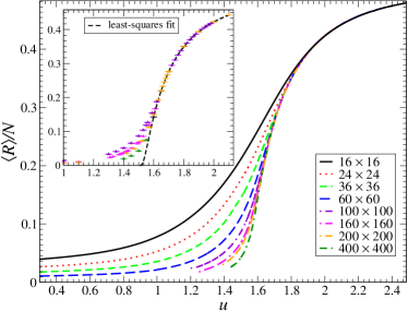
Figure 3: (color online) The orientational order parameter $R$ in the undoped case: it vanishes for $u<u_{c}$ and has an essential singularity at $u_{c}$. The curves represent Monte Carlo data for different lattice sizes, interpolated via multiple histogram reweighting. Inset: data collapse, with a least-squares fit to the exact scaling function for the staggered polarization operator of the six-vertex model (61) related to $R$ by a universality mapping as discussed in the text.

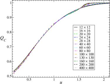
Figure 4: (color online) Fourth-order amplitude ratio of the columnar order parameter $C$ in the undoped case. The curves for all system sizes essentially coincide for the entire critical phase ($u<u_{C}$), as expected for a KT transition.

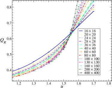
Figure 5: (color online) Fourth-order amplitude ratio of the orientational order parameter $R$ in the undoped case. In contrast to the amplitude ratio of the columnar order parameter $C$ (Fig. 4), this quantity exhibits a strong finite-size dependence, leading to an effective crossing point that can be used to locate the transition point.

For completeness, we also investigate the behavior of the fourth-order amplitude ratios $Q_{M}=\langle{M}^{2}\rangle^{2}/\langle{M}\rangle^{4}$ with $M=C$, $R$. The behavior of $Q_{C}$, shown in Fig. 4, is similar to what is expected for the $XY$ model, namely a collapse of all curves in the critical low-$u$ phase and no well-defined crossing of curves for different system sizes. In contrast, $Q_{R}$ (Fig. 5) is found to exhibit such strong finite-size effects in the critical phase that its behavior almost resembles that of a regular continuous phase transition. This anomalous behavior explains why the crossing point of the curves for different system sizes could be exploited to obtain an accurate estimate of the critical couplingAlet et al. (2005, 2006). In the figures presented in this section, the multiple histogram reweighting methodFerrenberg and Swendsen (1989) has been used to interpolate all data obtained at different values for the coupling parameter. This allows us to accurately locate crossing points and extrema in the curves.

Alet and coworkersAlet et al. (2005, 2006) and Poilblanc and coworkersPoilblanc et al. (2006) used transfer-matrix calculations and Monte Carlo simulations to study the critical behavior of the undoped system for $u>0$ (attractive dimer interactions), whereas Castelnovo and coworkersCastelnovo et al. (2007) used transfer-matrix methods to study primarily the $u<0$ (“repulsive”) regime. In addition, in Ref. Alet et al., 2006 the doped interacting dimer model was also briefly studied for low doping by means of numerical transfer-matrix techniques. All these results are consistent and complementary to those presented in the following subsection.

V.3 Low doping: Line of fixed points

We now proceed to the low-doping regime. We perform simulations in the canonical ensemble, for couplings near the critical region and for hole densities $\rho_{h}=0.004,0.01,0.02,0.04,0.06$. Figure 6 shows, for $\rho_{h}=0.06$, the susceptibilities of the columnar and orientational order parameters, $C$ and $R$, followed by the corresponding fourth-order amplitude ratios in Fig. 7.

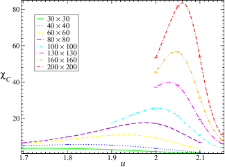
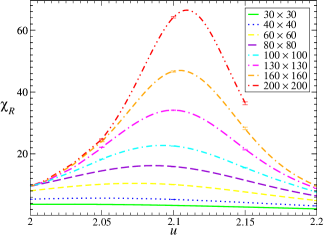
Figure 6: (color online) Classical susceptibilities of (a) the columnar order parameter $C$ and (b) the orientational order parameter $R$, for $\rho_{h}=0.06$. The magnitude and position of the maxima for different lattice sizes $L$ can be used to extract the critical exponents $\gamma$ and $\nu$.

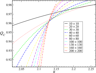
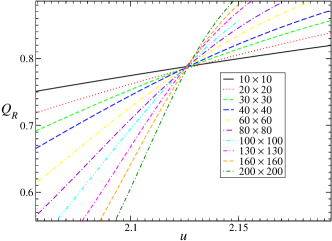
Figure 7: (color online) Fourth-order amplitude ratios of (a) the columnar order parameter $C$ and (b) the orientational order parameter $R$, for $\rho_{h}=0.06$. The clear crossings of the curves for different system sizes indicate a regular continuous phase transition.

According to the predictions of Section IV.2, we expect that the columnar order parameter $C$, which maps onto the $O_{1,0}$ effective operator in the scaling limit, will retain its scaling dimension $1/8$ along the critical line that emerges from the KT transition point for low hole doping and which constitutes the phase boundary between the dimer-hole liquid and the columnar solid phases. This constant value of the scaling dimension of $C$ is the most salient signature of this critical line: The scaling dimensions of all the other operators change continuously along the phase boundary.

To test this prediction, we extract the anomalous dimensions $\eta_{C}$ and $\eta_{R}$ (which are equal to twice their scaling dimension) by means of finite-size scaling. The maximum of the susceptibility scales as $\chi^{\rm max}\sim L^{2-\eta}+\cdots$. Subleading scaling contributions are omitted in the fitting expression since the results for sufficiently large lattice sizes satisfy simple scaling [cf. Figs. 8 and 9].

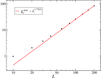
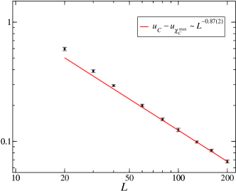
Figure 8: (color online) Finite-size scaling analysis of the susceptibility of the columnar order parameter $C$ for $\rho_{h}=0.06$: (a) Scaling of the height of the maximum as a function of system size $L$. (b) Scaling of the position of the maximum. The critical value $u_{c}$ is obtained from the crossing of the fourth-order cumulants (cf. Fig. 7). The same power-law behavior of the susceptibility maximum is found for all hole densities $\rho_{h}\leq 0.06$.

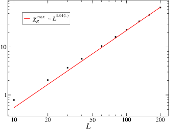
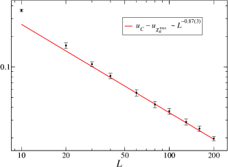
Figure 9: (color online) Finite-size scaling analysis of the susceptibility of the orientational order parameter $R$ for $\rho_{h}=0.06$: (a) Scaling of the height of the maximum as a function of system size $L$. (b) Scaling of the position of the maximum. The critical value $u_{c}$ is obtained from the crossing of the fourth-order cumulants (cf. Fig. 7). Unlike the results for the columnar order parameter (Fig. 8) the power-law behavior of the susceptibility maximum is is now dependent on the hole density, consistent with an anomalous scaling exponent that varies along the phase boundary.

The correlation-length exponent $\nu$ can be extracted from the slope of the fourth-order amplitude ratios of both order parameters at the critical point. Here, instead, we obtain it from the scaling behavior of the location of susceptibility maximum, which scales as $u_{\chi^{\rm max}}=u_{c}+{\rm const.}\;L^{-1/\nu}+\cdots$ (cf. Figs. 8 and 9). The critical coupling $u_{c}$, in turn, is obtained from the crossing points of the fourth-order amplitude ratio (Fig. 7).

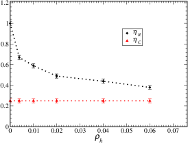
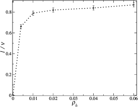
Figure 10: (a) Evolution of the anomalous dimensions $\eta_{C}$ (lower curve) and $\eta_{R}$ (upper curve) for the columnar and orientational order parameters, respectively, along the critical line for hole densities $0.004\leq\rho_{h}\leq 0.06$. The transition will become first-order when the two curves cross. (b) The inverse correlation-length exponent $1/\nu$ as a function of doping along the critical line for hole densities $0.004\leq\rho_{h}\leq 0.06$. Up to small systematic deviations discussed in the text, the observed trend agrees with the scaling predictions.

By repeating this procedure for different hole densities, we find $\eta_{C}$ and $\eta_{R}$, as well as $\nu$ as a function of $\rho_{h}$. We note that for the undoped case the (logarithmic) finite-size corrections are so strong that the anomalous exponents are very difficult to determine. By including subleading corrections to the susceptibility expressions at the KT transition, we find strong indications that $\eta_{C}=1/4$ and $\eta_{R}=1$, satisfying the established theoretical description of this KT transition. The density dependence of the exponents is shown in Fig. 10. Clearly, they behave very differently: For the columnar parameter $C$, its anomalous dimension remains unchanged and equal to $1/4$, while for $R$ it decreases monotonically from $1$ to $1/4$ where the transition is expected to become first-order, according to the scenario presented in Section IV.2. The results from our Monte Carlo simulations are thus consistent with the predictions we made in our theoretical analysis.

The evolution of the correlation length exponent along the phase boundary is shown in Fig. 10. This exponent behaves qualitatively as predicted for finite doping, i.e., it exhibits a monotonically decreasing behavior along the line of fixed points. A direct quantitative comparison to the field-theoretical prediction is not possible, since the simulations are performed in the canonical ensemble. Even though the dimer density could be mapped to a dimer fugacity, the field theory assumes a fixed hole fugacity. In addition, the evolution of the exponent in Fig. 10 is slower than predicted because in the simulations we do not approach the phase boundary perpendicularly in the simulations, which leads to an effective exponent $\nu$ that is smaller than the one computed from the scaling dimension of the relevant operator in the field theory.

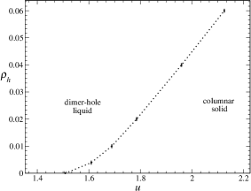
Figure 11: Phase diagram at low doping, with the critical line of fixed points separating the dimer-hole liquid phase [$u<u_{c}(x)$] from the columnar solid [$u>u_{c}(x)$].

In Fig. 11 we summarize our results for the location of the phase boundary between the dimer-hole liquid phase and the columnar solid phase for hole densities $\rho_{h}\leq 0.06$. The behavior of the critical line for $\rho_{h}\to 0$ is consistent with its expected scaling behavior $\rho_{h}\propto\xi^{-2}(\rho_{h}=0)$ which is based on simple dimensional analysis, with the only length scale of the problem being the correlation length of the undoped problem.

V.4 High doping: First Order Transition and Phase Separation

Beyond the multicritical point predicted in Sections III and IV.2 (see also Appendix A), we expect a first-order transition line in the $z_{d}$–$u$ phase diagram, where $z_{d}$ denotes the dimer fugacity. This line separates the crystalline from the liquid phase. According to our scenario, an entropic attraction between holes on the same sublattice becomes marginal and leads naturally to phase separation between a hole-rich liquid phase and a hole-poor columnar crystalline phase. Since the multicritical point is characterized by a marginally relevant operator, complicated crossover will be observed in the first-order transition region in the vicinity of this point.Cardy et al. (1980) In addition, close to the multicritical point, the first-order transition will be very weak, with a discontinuity that vanishes with an essential singularity as a function of the distance to the multicritical point along the phase coexistence curve. At this transition, all observables, such as the latent heat, should vanish in a similar way, making the numerical study of the transition close to the multicritical point particularly difficult.

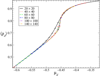
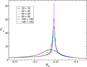
Figure 12: (color online) (a) The $\rho_{d}$–$\mu_{d}$ equation of state for coupling $u=3.5$ and different lattice sizes. As the system size increases, the jump in the dimer density at the first-order phase transition gradually becomes more pronounced, but remains relatively weak. (b) The heat capacity of the classical interacting dimer model for the same coupling strength. We find that the peak scales as $C_{\rm max}\sim C_{0}+L^{2}$, providing strong evidence for a first-order transition at $u=3.5$.

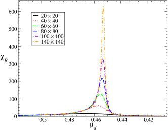
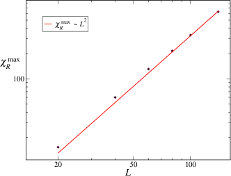
Figure 13: (color online) (a) Susceptibility of the orientational order parameter $R$ for coupling $u=3.5$ and different lattice sizes. (b) Asymptotically, the maxima of $\chi_{R}$ scale with the lattice size, confirming the first-order nature of the phase transition.

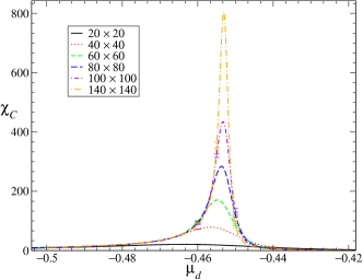
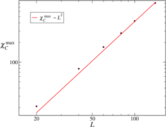
Figure 14: (color online) (a) Susceptibility of the columnar order parameter $C$ for coupling $u=3.5$. (b) The maxima of $\chi_{C}$ as a function of the linear lattice dimension. As for $\chi_{R}$ (Fig. 13), the maxima scale with lattice size, supporting the occurrence of a $\delta$-function singularity in $\chi_{C}$ in the thermodynamic limit, as expected for a first-order phase transition.

To confirm the existence of the discontinuous transition we perform grand-canonical Monte Carlo simulations with single-dimer insertions and deletions (alternated with canonical geometrical cluster moves to accelerate the relaxation of the configurations), for couplings $u=3.0$, $3.5$, $4.0$, $5.0$, $6.0$, as a function of the dimer fugacity $z_{d}$. Figure 12 shows the dimer density as a function of dimer chemical potential $\mu_{d}$. Although with increasing system size a jump in the dimer density develops, it does not become very pronounced. However, consideration of the heat capacity $C_{V}$ [Fig. 12] confirms the presence of a single phase transition at fixed coupling constant $u$, as $C_{V}$ exhibits a peak at a chemical potential that matches the location of the jump in $\rho_{d}$. We emphasize that this classical heat capacity is not the heat capacity of the $(2+1)$-dimensional QDM. Indeed, $C_{V}$ does not have any physical meaning in terms of the ground-state wave function that we are considering, because the ground-state energy cannot be changed through variation of the parameters $u$ or $\mu_{d}$. Another confirmation of the phase transition is obtained from the susceptibilities of the orientational [Fig. 13] and columnar [Fig. 14] order parameters, $\chi_{R}$ and $\chi_{C}$, respectively. Both quantities exhibit a peak at a chemical potential that approaches, with increasing system size, the location of the peak observed in $C_{V}$.

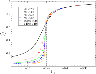
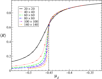
Figure 15: (color online) (a) The columnar order parameter $C$ as a function of the dimer chemical potential $\mu_{d}$ for coupling $u=3.5$. The rapid increase near the transition becomes more pronounced as the thermodynamic limit is approached. The dashed line shows the approximate position of the transition point. (b) The orientational order parameter $R$ as a function of the chemical potential $\mu_{d}$ for coupling $u=3.5$. It also shows a rapid increase similar to the behavior of $C$, at the same chemical potential.

To confirm the nature of the phase transition, we consider the scaling of the peaks in $C_{V}$, $\chi_{R}$, and $\chi_{C}$. For a first-order transition, these quantities should exhibit a $\delta$-function singularity in the thermodynamic limit or equivalently, for finite systems their peaks must scale with the lattice size in a finite system. We find that the heat-capacity peak, apart from a constant background, indeed scales with the lattice size $L^{2}$ for the range of system sizes (up to $L=140$) that we considered. This is supported by the behavior of the system-size dependent maxima in $\chi_{R}$ and $\chi_{C}$, see Figs. 13 and 14, which both scale as $L^{2}$, indicating that $\eta=0$. In addition, all local order parameters must develop a discontinuity at the transition point as the system size increases. Whereas the jump in the dimer density [Fig. 12] is not very sharp, the jump in the columnar and orientational order parameters, $C$ and $R$, is quite pronounced already for the system sizes studied here, see Figs. 15 and 15. Furthermore, the location the order-parameter jump provides a good indication of the transition point.

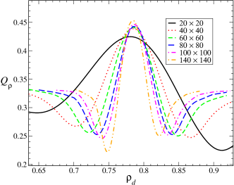
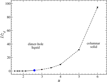
Figure 16: (color online) (a) Fourth-order amplitude ratio for the dimer density, at coupling $u=3.5$. The exhibited behavior is typical of a first order transition.Kim et al. (2003), with two minima that in the thermodynamic limit approach the coexisting densities. (b) Phase boundary between the dimer liquid and the columnar solid. For low couplings, the transition is continuous (solid line). Our best estimate for the multicritical point ($u_{c}\approx 2.6$) is represented by the large circular dot. Beyond the multicritical point, the phase boundary (dashed line) is estimated from grand-canonical MC simulations at fixed dimer fugacity $z_{d}$.

The strongest evidence, however, is provided by the fourth-order amplitude ratio of the density, $Q_{\rho}$. At a first-order transition, this quantity displays a specific behavior, as discussed in Ref. Kim et al., 2003. In particular, the positions of two minima observed in Fig. 16 approach, in the thermodynamic limit, the densities of the two coexisting phases. Outside the coexistence region, $Q_{\rho}$ approaches a limiting value $1/3$, characteristic of Gaussian fluctuations. This type of behavior is not found at a continuous phase transition, and should be considered as a strong indicator for the occurrence of a first-order transition. This is particularly important since the very weak nature of the first-order transition makes it impossible to unambiguously confirm the existence of a double peak in the histograms of the internal energy for the system sizes that we considered. Whereas the first-order transition becomes more pronounced at higher couplings, and it thus should become easier to distinguish the two peaks in the energy histogram, in practice those simulations are seriously hampered by the very large relaxation times encountered for large dimer interactions.

By repeating the analysis presented here for different couplings, and estimating the coexistence chemical potential from the convergence point observed at the order-parameter discontinuity (cf. Fig. 15), we derive the phase diagram in the $z_{d}$–$u$ plane, see Fig. 16.

VI Effects of repulsive hole-hole interactions near the first-order transition region

We now discuss briefly the effects of additional interactions near the coexistence curve. It is clear that additional interactions near the first-order transition line should stabilize more complex ordered inhomogeneous phases. The simplest interaction that competes with the tendency of holes to pair and phase separate from the crystal is a weak nearest-neighbor hole-hole repulsion $V_{h}$. The addition of such an interaction to the classical dimer model would lead to an additional energy cost for homogeneous and isotropic clusters of holes. Remarkably, for a range of dimer interactions $u$, this energy cost leads to the formation of commensurate hole stripes with period $3$, in a region in the phase diagram located between the dimer-columnar crystal and the hole-dimer liquid. For general values of $u$, $V_{h}$ and hole densities one expects a complex phase diagram, most likely similar to what is found in theories of commensurate-incommensurate transitions, which we do not explore here in detail but are discussed in Refs. Pokrovsky and Talapov, 1978; Bak, 1982; Fisher and Selke, 1980; Papanikolaou et al., 2007.

This phase can be thought of as the ground-state wave function of a quantum Hamiltonian constructed using the approach described in Section II. The quantum Hamiltonian that leads to the prescribed wave function includes a generalized form of the hole-related Hamiltonian of Eq. 6,

$$H=H_{d}+t_{\rm hole}\sum_{i}\Bigg{[}-\Big{|}C^{h}_{i}\Big{>}\Big{<}C^{h^{\prime}}_{i}\Big{|}-\Big{|}C^{h^{\prime}}_{i}\Big{>}\Big{<}C^{h}_{i}\Big{|}$$

$$+y^{R_{C^{h^{\prime}}_{i}}-R_{C^{h}_{i}}}\Big{|}C^{h}_{i}\Big{>}\Big{<}C^{h}_{i}\Big{|}+y^{R_{C^{h}_{i}}-R_{C^{h^{\prime}}_{i}}}\Big{|}C^{h^{\prime}}_{i}\Big{>}\Big{<}C^{h^{\prime}}_{i}\Big{|}\Bigg{]}\;,$$ (62)

where $R_{C_{i}^{h}}$ and $R_{C_{i}^{h^{\prime}}}$ denote the number of pairs of holes formed in the corresponding configurations $C_{i}^{h}$ and $C_{i}^{h^{\prime}}$ (cf. Fig. 17). More specifically, the ground-state wave function is

$$|G^{int}_{N_{h}}\rangle=\frac{1}{\sqrt{Z(w^{2},y^{2},N_{h})}}\sum_{\{\mathcal{C}_{N_{h}}\}}w^{\displaystyle{N^{d}_{p}[\mathcal{C}_{N_{h}}]}}y^{\displaystyle{N^{h}_{p}[\mathcal{C}_{N_{h}}]}}|\mathcal{C}_{N_{h}}\rangle\;.$$ (63)

This wave function has a counterpart in the grand-canonical ensemble, for which the exactly solvable quantum Hamiltonian is a generalization, in exactly the same way as above, of Eq. (8).

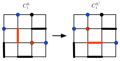
Figure 17: (color online) A particular hopping process realized in the Hamiltonian Eq. (62). The potential terms that are present in the Hamiltonian depend on the number of additional pairs of holes that are formed after the hopping process. In the process shown above, this number is 1.

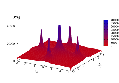
Figure 18: (color online) The hole density structure factor $S(k)$ for dimer coupling $u=5.0$, hole repulsion $V_{h}=0.5$ and dimer chemical potential $\mu_{d}=-1.0$, for linear system size $L=128$. The four peaks at $(\pm 2\pi/3,0)$ and $(0,\pm 2\pi/3)$ correspond to the ordered configuration of hole-stripes shown in Fig. 19.

Figure 19: Snapshot of a part of a typical ordered configuration that appears at the couplings $u=5.0$, $V_{h}=0.5$, $\mu_{d}=-1.0$ and linear system size $L=128$. Holes prefer to form commensurate stripes of period $3$, so as to minimize the effect of the weak hole repulsions.

By performing grand-canonical simulations for weak hole repulsions $V_{h}\leq\frac{1}{10}u$ in the regime of strong dimer attractions, $u>4.0$, where the first-order transition is more pronounced, a hole-stripe phase was observed. In particular, for the couplings $u=5.0,V_{h}=0.5$ and a dimer chemical potential $-1.1<\mu_{d}<-0.8$ (i.e., between the liquid phase $\mu_{d}\lesssim-1.2$ and the columnar phase $\mu_{d}\gtrsim-0.8$), the hole density structure factor shows non-trivial peaks at $(k_{x},k_{y})=(\pm 2\pi/3,0),(0,\pm 2\pi/3)$, which sharpen as the lattice size increases (see Fig. 18). A snapshot of the ordered phase (Fig. 19) illustrates how the holes order in stripes with a period of three lattice spacings, whereas the dimers are still ordered in a columnar pattern. In this way, the holes minimize the effect of the hole-hole repulsions and the dimers simultaneously maximize the effect of the attractive dimer-dimer interactions. The same pattern is also found for $u=4.0,4.5,6.0$, in similar regimes for the hole-hole interaction.

More generally, we expect that, as the liquid phase is approached in the regime of strong dimer couplings, a sequence of hole-commensurate phases will be stabilized, leading ultimately to incommensurate phases next to the liquid phase. The formation of this phase diagram is similar in spirit to the ones discussed in Refs. Pokrovsky and Talapov, 1978; Bak, 1982; Fisher and Selke, 1980; Papanikolaou et al., 2007.

VII Elementary quantum excitations of doped quantum Dimer Models

In the preceding two sections we discussed the properties of the ground-state wave functions and the behavior of equal-time correlation functions of several operators of physical interest. There we used extensively the connection that exists for these type of wave functions between the computation of equal-time correlators of local operators and computations of similar objects in the equivalent two-dimensional classical statistical mechanical system of interacting dimers and holes. In this section we will be interested in the spectrum of low lying excitations which is inherently a quantum mechanical property.

Unfortunately, as it usually the case in QDMs,Rokhsar and Kivelson (1988) all we know is the ground-state wave function. The low-lying excitation spectrum is not known exactly but it can be computed approximately using the variational principle. This is the single mode approximation (SMA), which is a useful tool for studying the excited states of many body systems.Feynman (1972); Mahan (1990); Arovas and Girvin (1991); Girvin et al. (1985); Arovas et al. (1988) It is particularly useful in the case of quantum dimer models at their RK points due to the fact that the exact ground-state wave function is known exactly. The computation of the low lying collective modes in the QDM was done by Rokhsar and Kivelson.Rokhsar and Kivelson (1988) Alternatively, one can describe qualitatively the low-lying spectrum using the effective field theory of the quantum dimer models (and their generalizations) at criticality, the quantum Lifshitz model of Ref. Ardonne et al., 2004.

In this section we will consider only the SMA spectrum in the dimer-hole liquid phase. Similar calculations can be done in the phase with long-range columnar order. In the dimer-hole liquid phase the equal-time correlation function of the hole density operator, i.e. the one-body density matrix, approaches a constant at long distances. Thus the wave function for this phase exhibits a Bose condensate of holes. Since the holes are charged, this is a charge Bose condensate. To determine if it is a superfluid (or more precisely a superconductor) it is necessary to show that it has a finite superfluid stiffness, i.e. a critical velocity. This can be determined form the spectrum of density fluctuations and hence from the spectrum of collective modes. It will turn out that, in spite of the more correlated nature of the wave functions we consider here, the result will be similar to that of Rokhsar and Kivelson,Rokhsar and Kivelson (1988) i.e. no superfluid stiffness. Given the more general structure (while still local) of the wave functions we study here, we conclude that wave functions associated with Hamiltonians satisfying the RK condition in general do not describe superfluid states.

We begin by summarizing the SMA procedure, focusing on doped quantum dimer models. Firstly, one must know the exact ground state of the system $|0\rangle$ and the type of excitations which saturate the frequency sum rule. In our case, there are two candidates: the dimer density and the hole density excitations. Since it follows from a variational principle, the SMA provides a proof of existence only for gapless excitations but not for gapped ones. The energy of an excitation created by an operator with wave vector $\bf k$, which we will denote by $\hat{\rho}_{\bf k}$, acting on the ground state is bounded from above as followsFeynman (1972); Mahan (1990); Arovas and Girvin (1991)

$$E_{\bf k}-E_{0}\leq\frac{f(\bf k)}{s(\bf k)}=\frac{\langle 0|\left[\hat{\rho}(-\bf k),\left[\cal{H},\hat{\rho}(\bf\bf k)\right]\right]|0\rangle}{\langle 0|\hat{\rho}(-\bf k)\hat{\rho}(\bf k)|0\rangle}\;,$$ (64)

where $f(\bf k)$ is the “oscillator strength” and $s(\bf k)$ is the structure factor (i.e. the equal-time correlation function) for the operator $\hat{\rho}(\bf k)$.

In the case of doped QDMs at their RK point we know their ground-state wave functions exactly and they have (by construction) zero ground-state energy, $E_{0}=0$. Thus the excitation spectrum must be positive. The system will have gapless excitations if $E_{\bf k}-E_{0}$ vanishes at some wave vector. It is worth noting that there are two distinct ways for the SMA bound to vanish close to some ${\bf k}={\bf k}_{0}$. One way is if $f(\bf k)$ vanishes at ${\bf k}_{0}$. This can happen only if the commutator $\left[\cal{H},\hat{\rho}({\bf k}_{0})\right]$ vanishes. This means that $\rho({\bf k}_{0})$ is a conserved quantity. The other way occurs when $s(\bf k)$ becomes infinite at ${\bf k}_{0}$. This is a signature of a nearby density-ordered state like the columnar dimer crystal we found in the phase diagram of the dimer models under study, shown in Fig. 2.

In the following, we will use the following operator definitions. For dimers, $\hat{\sigma}_{\hat{\alpha}}^{d}({\bf r})$ denotes the dimer density operator and it takes the values $\pm 1$ if a dimer is present or absent at the link which begins at the position ${\bf r}$ and has direction $\hat{\alpha}=\hat{x},\hat{y}$. For holes, $\hat{\sigma}^{h}({\bf r})$ denotes the hole density operator and it takes the values $\pm 1$ if a hole is present or absent at the position ${\bf r}$.

Details of the derivations of the SMA oscillator strength functions for both models are given in Appendix B. Here we just quote the main results.

VII.1 The fixed hole density model

VII.1.1 Hole density excitations

For the fixed hole density model the SMA oscillator strength function $f(\bf k)$ for hole density excitations is given by

$$f({\bf k})=4t_{\rm hole}{\bf q}^{2}$$ (65)

for ${\bf k}=(\pi,\pi)+\bf q$.

From the results of the Section III and Appendix A, we may conclude that: For ${\bf k}=(\pi,\pi)+{\bf q}$, the structure factor near $(\pi,\pi)$ scales like $s^{(\pi,\pi)}({\bf k})\propto\frac{1}{q^{2}+\xi^{-2}}$ and thus, $s^{(\pi,\pi)}(0)$ is a constant. Thus $E_{\bf k}^{(\pi,\pi)}-E_{0}\propto{\bf q}^{2}$. For ${\bf k}=(0,0)+{\bf q}$, the results from the following section, which formally hold only for low density of dimers, lead to the conclusion that $s^{(0,0)}({\bf k})\propto\frac{1}{q^{2}-\xi^{-2}}$ and $s^{(0,0)}(0)$ is again a constant but has strong oscillatory behavior in real space. Thus, from the correlation function we computed in and Appendix A, we conclude that these excitations are also quadratic in the momentum ${\bf q}$, i.e.,  $E_{\bf k}-E_{0}\leq{\bf q}^{2}$. This result is consistent with the compressibility argument, given in Ref. Rokhsar and Kivelson, 1988 which would also give quadratic dispersion in this case (keeping in mind that in this case the compressibility is infinite when the system is doped (constant number of holes)). However, it is important to stress that the compressibility argument is a stronger condition because our calculation of the correlation function is legitimate for low dimer densities.

VII.1.2 Dimer density excitations

For the fixed hole density model the SMA oscillator strength function $f(\bf k)$ for dimer density excitations is given by

$$f({\bf k})=f_{\rm dimer-flip}({\bf k})+f_{\rm hole(1)}({\bf k})$$ (66)

Close to the wave vector ${\bf Q}_{0}=(\pi,\pi)$ with ${\bf k}={\bf Q}_{0}+{\bf q}$, both oscillator strengths $f_{\rm dimer-flip}({\bf k})$ and $f_{hole(1)}$ vanish quadratically (cf. Appendix B) and more specifically,

$$f_{\rm dimer-flip}({\bf q})=8tq^{2}$$ (67)

$$f_{\rm hole(1)}({\bf q})=-t_{\rm hole}q^{2}$$ (68)

Given the fact that the dimer density structure factor is a constant at $Q_{0}=(\pi,\pi)$ and combining Eqs.(131) and (66), we may conclude that there are gapless dimer density excitations at $Q_{0}=(\pi,\pi)$.

In addition to these results, we may have additional branches of dimer density excitations, specially when there is a divergence of the structure factor at some wave vector ${\bf Q}_{0}$ which would would be an indication of dimer order at a nearby phase. In particular, this happens at the phase boundary between the hole-dimer liquid phase and the columnar-ordered crystalline phase.

VII.2 The fixed hole fugacity model

As above, we can study the hole density excitations of the second model, the grand-canonical model, in which the hole density is not fixed, but is determined by a parameter $z$ which plays the role of a hole fugacity in the wave function. By the fact that there is no conservation of the number of holes is explicitly broken, we can predict that the numerator $f({\bf k})$ will vanish only at ${\bf Q}_{0}=(\pi,\pi)$. This happens because of the bipartite lattice symmetry that enforces the number holes on each sublattice to be equal. For the fixed hole fugacity model the SMA oscillator strength function $f(\bf k)$ for hole density excitations is

$$f_{\rm hole(2)}({\bf k})=4t_{\rm pairing}(2+\cos({\bf k}_{x})+\cos({\bf k}_{y}))$$ (69)

The formula shows that the numerator $f_{\rm hole(2)}({\bf k})$ vanishes only at the wave vector ${\bf Q}_{0}=(\pi,\pi)$ quadratically, as expected. The dimer density excitations are not gapless (in the sense that the numerator does not vanish for any ${\bf Q}_{0}$) because the dimer-flip contribution vanishes at $(\pi,\pi),(0,\pi)$ and the dimer-breaking term gives a constant contribution. This is expected due to the violation of the dimer number conservation. It is important to stress that the behavior of the structure factor is exactly the same as before (in the fixed hole-density model). The reason is the equivalence of the canonical and grand-canonical ensemble in the thermodynamic limit for classical systems.

It is certainly worth noting that, although the two ground-state wave functions of Eqs. (7) and (9) have the same ground-state physics, due to the essential equivalence of the classical canonical and grand-canonical ensembles in the thermodynamic limit, the nature of their quantum elementary excitations is drastically different.

VIII Conclusions

In this work we have constructed generalizations of the quantum dimer model to include the effects of dimer correlations as well as finite hole doping in the wave function. Throughout we considered the case of bosonic (charged) holes and neglected the fermionic spinons. We have constructed generalized RK Hamiltonians whose ground-state wave functions describe the effects of (attractive) dimer correlations and finite hole doping. We have discussed the rich phase diagram and critical behavior of three doped interacting quantum dimer models at their RK point using both analytic methods and numerical simulations. We have shown that the ground-state wave function embodies a complex phase diagram which consists of dimer-hole liquid and columnar phases separated by a critical line with varying exponents, ending at a multicritical point with a Kosterlitz-Thouless structure where the transition becomes first order. The critical behavior along the low doping section of the phase boundary was investigated in detail and the predictions of our scaling analysis were confirmed with large-scale Monte Carlo simulations. Monte Carlo simulations were also used to show that the transition between the dimer-hole liquid and the columnar solid does indeed become first order, and to estimate the location of the multicritical point and of the first-order phase boundary.

In the high-doping regime, near the first-order transition line, additional repulsive interactions among holes were shown to generate, at the expense of the two-phase region, an even richer phase diagram with phases in which the dimer-hole system becomes inhomogeneous. In the regime of strong dimer coupling, $u=5=0.$, and weak hole interactions, $V_{h}=0.5$, we found a stripe phase with wave vectors $(2\pi/3,0)$ and $(0,2\pi/3)$. In general, we expect the two-phase region to be replaced by a complex phase diagram with a large number of commensurate and incommensurate phases. This physics is well known in the context of two-dimensional classical statistical mechanics of systems with competing interactions.Pokrovsky and Talapov (1978); Bak (1982); Fisher and Selke (1980) However, it is interesting to see how it arises at the level of the exact ground-state wave function of models of strongly correlated systems, particularly given the current interest on this type of phenomena in high-temperature superconductors and related systems.Zaanen and Gunnarsson (1989); Kivelson and Emery (1994); Kivelson et al. (1998); Emery et al. (1999); Sachdev (2003); Balents et al. (2005)

In this paper we have also presented an analysis of the low-lying excitations of the quantum system and found that, much as in the case of the Rokhsar-Kivelson quantum dimer model, the doped system is a Bose-Einstein condensate but not a superfluid, since the superfluid stiffness vanishes even though both dimers and holes interact. It is apparent that in order to render the Bose-Einstein condensate a true superfluid it is necessary to violate the RK condition which forces the wave function to have a local structure. The effects of violations to the RK condition are poorly understood, and we have not investigated this important problem which is essential to determine the generic phase diagram of these models.

Appendix A Mean-Field Theory for dimers and holes

In this Appendix we give details of the mean-field theory summarized in Section III. We will use Grassmann variable methods to write down the partition functions for classical interacting and doped dimers. We will use these methods to derive a simple mean-field theory for this system. While mean-field theory, as it is well known, fails to give the correct critical behavior in two-dimensional systems, it offers a good qualitative description of the phases and, surprisingly, even of the gross features of the phase diagram. In subsequent sections we will use more sophisticated analytic and numerical methods to study the phase transitions.

A.1 Non-Interacting dimers at finite hole density

The classical dimer-hole partition function can be formulated in terms of a Grassmann functional integral, according to the prescription of Ref. Samuel, 1980b. The classical partition function of the dimer problem on any lattice which is defined by the connectivity matrix $M$ and with fugacity $z$ for the dimers and 1 for the holes is:

$$\mathcal{Z}_{\rm dimer} = \int\mathcal{D}\eta\mathcal{D}\eta^{\dagger}e^{\sum_{i}\eta_{i}\eta^{\dagger}_{i}+\frac{z}{2}\sum_{ij}M_{ij}\eta_{i}\eta_{i}^{\dagger}\eta_{j}\eta_{j}^{\dagger}}$$

For the square lattice, $M_{ij}$ is 1 if $i,j$ are nearest neighbor sites and zero otherwise. For the triangular lattice, $M_{ij}$ is 1 if $i,j$ are nearest neighbors and also next-nearest neighbor sites, but only along one diagonal, i.e., if $j=i+\hat{\bf{x}}+\hat{\bf{y}}$ or $j=i-\hat{\bf{x}}-\hat{\bf{y}}$. Also, the fugacity z ranges from 0 to $\infty$. When $z\rightarrow 0$, the system is filled with holes and there are very few dimers and when $z\rightarrow\infty$ the system approaches the close-packed limit with dimers. Both limits are worth of study due to the existence of an important theorem by Heilmann and LiebHeilmann and Lieb (1970) which proves under rather general assumptions the absence of any phase transitions with doping in this model. Thus, the identification of the phase in the few dimers limit is enough to conclude about the phase that the system enters when doped. In this section we will study this problem in the limit in which the dimers are dilute. In this regime a simple mean-field theory of the Hartree type is expected to be accurate.Samuel (1980b) Such a crude approximation should break near criticality, i.e. near the close packing limit.

To proceed, we apply a Hubbard-Stratonovich transformation to the above partition function:

$$e^{\frac{z}{2}\sum_{ij}M_{ij}\eta_{i}\eta_{i}^{\dagger}\eta_{j}\eta_{j}^{\dagger}} = \mathcal{N}\int\mathcal{D}\phi e^{-\frac{1}{2z}\sum_{ij}\phi_{i}M^{-1}_{ij}\phi_{j}+\sum_{i}\eta_{i}\eta_{i}^{\dagger}\phi_{i}}$$

where $\mathcal{N}$ is an irrelevant normalization constant. We may also add sources for the hole density operators $J\eta\eta^{\dagger}$. In this way, the classical dimer partition function may be written as follows:

$$\mathcal{Z}_{\rm dimer} = \int\mathcal{D}\phi\mathcal{D}\eta\mathcal{D}\eta^{\dagger}e^{-\frac{1}{2z}\sum_{ij}\phi_{i}M^{-1}_{ij}\phi_{j}+\sum_{i}\eta_{i}\eta_{i}^{\dagger}(\phi_{i}+1+J_{i})}$$

where he have dropped the normalization constant $\mathcal{N}$, as we will do in what follows. (Note that what makes the above problem unsolvable is the term ‘1’ in the exponent!)

Upon integrating out the Grassmann variables we find:

$$\mathcal{Z}_{\rm dimer} = \int\mathcal{D}\phi\;e^{-\frac{1}{2z}\sum_{ij}(\phi_{i}-J_{i})M^{-1}_{ij}(\phi_{j}-J_{j})+\sum_{i}\ln(\phi_{i}+1)}$$

In the limit $z\rightarrow 0$ we may formulate a legitimate and well-defined mean-field theory. To this end we rewrite the partition function in the following way:

$$\mathcal{Z}_{\rm dimer} = \int\mathcal{D}\phi\;e^{-\frac{1}{z}\left[\frac{1}{2}\sum_{ij}(\phi_{i}-J_{i})M^{-1}_{ij}(\phi_{j}-J_{j})-z\sum_{i}\ln(\phi_{i}+1)\right]}$$ (74)

$$= \int\mathcal{D}\phi\;e^{-\frac{1}{z}\mathcal{S}(\phi)}$$

where

$$S(\phi) = \frac{1}{2}\sum_{ij}(\phi_{i}-J_{i})M^{-1}_{ij}(\phi_{j}-J_{j})-z\sum_{i}\ln(\phi_{i}+1)$$

is the effective action. As $z\rightarrow 0$, we have a theory which has a well-defined saddle point and the perturbation around this point will be in powers of $z$ which plays the role of an effective coupling constant. In this way, we have a very fast convergent expansion.

The saddle-point is defined as follows:

$$\frac{\delta\mathcal{S}}{\delta\phi_{i}}\bigg{|}_{\phi_{i}=\bar{\phi}}=0$$ (76)

and we take the following equation for $\bar{\phi}$ :

$$\bar{\phi}_{i}=J_{i}+z\sum_{j}\frac{M_{ij}}{\bar{\phi}_{j}+1}$$ (77)

In this approximation, the density of holes is given by:

$$\rho_{i}=\langle\eta_{i}\eta^{\dagger}_{i}\rangle = \frac{\partial\ln\mathcal{Z}_{dimer}}{\partial J_{i}}$$ (78)

$$= -\frac{1}{z}\frac{\partial\mathcal{S}}{\partial J_{i}}$$ (79)

$$= \frac{1}{\bar{\phi}_{i}+1}$$ (80)

So, the source $J_{i}$ in terms of the density of the holes $\rho_{i}$, is given by:

$$J_{i} = \bar{\phi}_{i}-z\sum_{j}\frac{M_{ij}}{\bar{\phi}_{j}+1}$$ (81)

$$= \frac{1}{\rho_{i}}-z\sum_{j}M_{ij}\rho_{j}-1$$ (82)

The Legendre transform of the effective action $\mathcal{S}$ is:

$$\Gamma(\rho_{i}) = \frac{1}{z}\mathcal{S}(\bar{\phi}_{j}(\rho_{i}),J_{j}(\rho_{i}))+\sum_{i}J_{i}(\rho_{j})\rho_{i}$$

$$= -\frac{z}{2}\sum_{ij}\rho_{i}M_{ij}\rho_{j}+\sum_{i}\ln(\rho_{i})+\sum_{i}(1-\rho_{i})$$

We specialize now to the case of uniform hole density $\rho_{i}=\rho$ and also for the case of the square lattice where the number of nearest neighbors is $2D=4$ and assuming that the number of sites on the lattice is $N$. Then,

$$\Gamma(\rho) = -\frac{z}{2}(4N\rho^{2})+N\ln(\rho)+N(1-\rho)$$ (85)

At this level of approximation (“Hartree”) the equation of state becomes

$$J=-4z\rho+\frac{1}{\rho}-1$$ (86)

So, when the sources are set to zero, the density in terms of the fugacity, in the limit $z\rightarrow 0$, is:

$$\rho\; = \frac{2}{1+\sqrt{1+16z}}$$ (87)

As a check of the approximation, we may expand the result in the region of $z\rightarrow 0$, where the result should be $\rho\simeq 1$ for the hole density:

$$\rho\;=1-4z+O(z^{2})$$ (88)

Or, equivalently, for $\rho\to 1^{-}$,

$$z=\frac{1}{4\rho}\left(\frac{1}{\rho}-1\right)=\frac{1}{4}\left(1-\rho\right)+O((1-\rho)^{2})$$ (89)

The hole density-density correlation function can be obtained in the following way by using the Legendre transform:

$$\mathcal{G}_{ij} = \langle\eta_{i}\eta^{\dagger}_{i}\eta_{j}\eta^{\dagger}_{j}\rangle-\langle\eta_{i}\eta^{\dagger}_{i}\rangle\langle\eta_{j}\eta^{\dagger}_{j}\rangle$$ (90)

$$= \frac{\partial^{2}\ln Z_{dimer}}{\partial J_{i}\partial J_{j}}=\frac{\partial\rho_{i}}{\partial J_{j}}$$

and also,

$$\mathcal{G}_{ij}=\left[\frac{\partial^{2}\Gamma}{\partial\rho_{i}\partial\rho_{j}}\right]^{-1}$$ (91)

By using (LABEL:LegendreTransform) and (91), we have:

$$\left[\mathcal{G}_{ij}\right]^{-1}=\frac{\partial^{2}\Gamma}{\partial\rho_{i}\partial\rho_{j}}=-zM_{ij}-\delta_{ij}\frac{1}{\rho_{i}^{2}}$$ (92)

Since $M_{ij}$ is a function of the distance between sites and vanishes except for nearest neighbors, its Fourier transform is:

$$M(\vec{q}) = a^{2}\sum_{i}e^{-i{\bf q}\cdot({\bf r}_{i}-{\bf r}_{j})}M({\bf r}_{i}-{\bf r}_{j})$$ (93)

$$= 2a^{2}\sum_{\alpha=1}^{2}\cos q_{\alpha}a$$

Also, we set $a=1$ and finally the hole density connected correlation function is:

$$\mathcal{G}(\vec{q}) = \frac{1}{-\frac{1}{\rho^{2}}-2z\sum_{\alpha=1}^{2}\cos q_{\alpha}}$$ (94)

For momenta near ${\bf Q}=(\pi,\pi)$, ${\bf q}={\bf Q}+{\bf p}$, with ${\bf p}$ small, it becomes

$$\mathcal{G}({\bf p}+{\bf Q}) \simeq \;-\;\frac{\rho\xi^{-2}}{\xi^{-2}+{\bf p}^{2}}$$ (95)

where $\xi$ is the correlation length

$$\xi=\sqrt{\displaystyle{\frac{1-\rho}{4\rho}}}$$ (96)

Finally, the connected hole density correlation function (the structure factor) in real space for $\rho\to 1$ is:

$$\mathcal{G}(r) = \frac{(-1)^{r_{x}+r_{y}+1}}{\sqrt{\pi\xi r}}e^{-\xi r}\;\;\;\;\;\;$$ (97)

If we restore the units, the correlation length is $\xi=a\sqrt{\frac{1-\rho a^{2}}{4\rho a^{2}}}$.

Surprisingly, given how crude this approximation is, the result of Eq. (97) is consistent with the numerical results provided by Krauth and MoessnerKrauth and Moessner (2003) for much of the dimer density range they studied. Significant deviations are seen only upon approach of the close packing regime where the classical dimer model is critical and this mean-field calculation fails, e.g. the correlation length diverges as $\rho\to 0$ with exponent $1/2$, given by Eq. (96), (the mean-field value). The correct value of the exponent can be deduced from Table 1 and it is $1/(2-1/4)=4/7$ ($1/4$ being the scaling dimension of the hole operator for the non-interacting case.) As we show in Section IV.1 (and in Table 1), the dimension of the hole operator grows from the value $1/4$ for free dimers to a value of $2$ at the (Kosterlitz-Thouless) transition to the columnar state, where it should exhibit an essential singularity due to the marginality of the hole operator.

A.2 Adding interactions between dimers

Clearly, the mean-field method for the non-interacting dimer-hole system can be easily extended to dimer-hole systems with local interactions. In the case of attractive interactions between parallel dimers, the partition function of the monomer-dimer system should be

$$\mathcal{Z}_{\rm d-int}=\int\mathcal{D}\eta\mathcal{D}\eta^{\dagger}\exp\Bigg{(}\sum_{i}\eta_{i}\eta^{\dagger}_{i}+\frac{z}{2}\sum_{ij}M_{ij}\eta_{i}\eta_{i}^{\dagger}\eta_{j}\eta_{j}^{\dagger}$$

$$+\frac{V}{4}\sum_{ijkl}\tilde{M}_{ijkl}\eta_{i}\eta_{i}^{\dagger}\eta_{j}\eta_{j}^{\dagger}\eta_{k}\eta_{k}^{\dagger}\eta_{l}\eta_{l}^{\dagger}\Bigg{)}$$

where $V=z^{2}(e^{u}-1)$ for an attractive interaction of strength $u>0$ between parallel neighboring dimers. $M_{ij}$ represents the coordination array of the lattice and it takes the value $1$ when $i$ is nearest neighbor to $j$ and otherwise is zero. In the same respect, $\tilde{M}_{ijkl}$ takes the value $1$ only when $i,j,k,l$ are arranged on a square plaquette and is zero otherwise. The sums run along all possible lattice sites for each index. We may perform two Hubbard-Stratonovich transformations by introducing the fields $\chi,\phi$ and then we have (again, dropping all normalization constants):

$$\mathcal{Z}_{\rm d-int} =\int\mathcal{D}\eta\mathcal{D}\eta^{\dagger}\mathcal{D}\chi\exp\Bigg{[}\sum_{i}\eta_{i}\eta^{\dagger}_{i}-\frac{1}{V}\sum_{ijkl}\chi_{ij}(\tilde{M}_{ijkl})^{-1}\chi_{kl}+\sum_{ij}\eta_{i}\eta_{i}^{\dagger}\eta_{j}\eta_{j}^{\dagger}(\chi_{ij}+\frac{z}{2}M_{ij})\Bigg{]}$$ (99)

$$=\int\mathcal{D}\eta\mathcal{D}\eta^{\dagger}\mathcal{D}\chi\mathcal{D}\phi\exp\Bigg{[}-\frac{1}{V}\sum_{ijkl}\chi_{ij}\tilde{M}_{ijkl})^{-1}\chi_{kl}-\frac{1}{4}\sum_{i}\phi_{i}(\chi_{ij}+\frac{z}{2}M_{ij})^{-1}\phi_{j}+\sum_{ij}\eta_{i}\eta_{i}^{\dagger}(\phi_{i}+1)\Bigg{]}\;\;\;\;\;$$

$$=\int\mathcal{D}\chi\mathcal{D}\phi\exp\Bigg{[}-\frac{1}{V}\sum_{ijkl}\chi_{ij}(\tilde{M}_{ijkl})^{-1}\chi_{kl}-\frac{1}{4}\sum_{ij}\phi_{i}(\chi_{ij}+\frac{z}{2}M_{ij})^{-1}\phi_{j}+\sum_{i}\ln(\phi_{i}+1)\Bigg{]}$$

Just as we did above, we introduce a set of auxiliary sources $J_{ij}^{\chi}$ defined on links $ij$, and $J_{i}^{\phi}$ defined on sites $i$. The partition function now reads

$$\mathcal{Z}_{\rm d-int}[J^{\chi},J^{\phi}]=\int\mathcal{D}\chi\mathcal{D}\phi\;e^{\displaystyle{-\frac{1}{Vz}\mathcal{S}(\phi,\chi;J^{\phi},J^{\chi})}}$$ (100)

where the action now is:

$$\mathcal{S}(\phi,\chi;J^{\phi},J^{\chi}) = z\sum_{ijkl}(\chi_{ij}-J^{\chi}_{ij})(\tilde{M}_{ijkl})^{-1}(\chi_{kl}-J^{\chi}_{kl})$$

$$+\frac{Vz}{4}\sum_{ij}(\phi_{i}-J^{\phi}_{i})(\chi_{ij}+\frac{z}{2}M_{ij})^{-1}(\phi_{j}-J^{\phi}_{j})-Vz\sum_{i}\ln(\phi_{i}+1)$$

We define the densities conjugate to the fields $\phi_{i},\chi_{ij}$ as:

$$n_{i}=\frac{\partial\ln\mathcal{Z}_{d-int}}{\partial J_{i}^{\phi}}=\frac{1}{2}\sum_{j}(\chi_{ij}+zM_{ij})^{-1}\phi_{j},\qquad m_{ij}=\frac{\partial\ln\mathcal{Z}_{d-int}}{\partial J_{ij}^{\chi}}=\frac{2}{V}\sum_{kl}(\tilde{M}_{ijkl})^{-1}\chi_{kl}$$ (102)

Solving for the fields and replacing in Eq.(LABEL:act-int), we have finally for the effective potential or equivalently the Gibbs free energy :

$$\Gamma(z,V)=\frac{V}{4}\sum_{ijkl}m_{ij}\tilde{M}_{ijkl}m_{kl} + \sum_{ij}n_{i}\bigg{(}\frac{V}{2}\sum_{kl}\tilde{M}_{ijkl}m_{kl}+\frac{z}{2}M_{ij}\bigg{)}n_{j}$$

$$- \sum_{i}\ln\Bigg{[}2\sum_{j}\Bigg{(}\frac{V}{2}\sum_{kl}\tilde{M}_{ijkl}m_{kl}+\frac{z}{2}M_{ij}\Bigg{)}n_{j}+1\Bigg{]}$$

The ordered phase of dimers is expected to be a columnar one. So, for $m_{ij}=(-1)^{x_{i}}\delta_{i,j-\hat{x}}m+m_{0}$ and $n_{j}=n$, the free energy is:

$$\frac{\Gamma(z,V)}{N} = Vm^{2}+2Vm_{0}^{2}+4Vm_{0}n^{2}+2zn^{2}$$

$$-\frac{1}{2}\ln\Bigg{(}1+8n\bigg{(}V(\frac{m}{2}+m_{0})+\frac{z}{2}\bigg{)}\Bigg{)}-\frac{1}{2}\ln\Bigg{(}1+8n\bigg{(}V(-\frac{m}{2}+m_{0})+\frac{z}{2}\bigg{)}\Bigg{)}$$

Now, we proceed by solving two of the three extremal (saddle-point) equations:

$$\frac{\delta\Gamma}{\delta n}=0\quad{\rm and}\quad\frac{\delta\Gamma}{\delta m_{0}}=0$$ (105)

which take the explicit form

$$8Vm_{0}n+4zn-\frac{4\bigg{(}V(\frac{m}{2}+m_{0})+\frac{z}{2}\bigg{)}}{1+8n\bigg{(}V(\frac{m}{2}+m_{0})+\frac{z}{2}\bigg{)}}-\frac{4\bigg{(}V(-\frac{m}{2}+m_{0})+\frac{z}{2}\bigg{)}}{1+8n\bigg{(}V(-\frac{m}{2}+m_{0})+\frac{z}{2}\bigg{)}}=0$$ (106)

$$4Vm_{0}+4Vn^{2}-\frac{4nV}{1+8n\bigg{(}V(-\frac{m}{2}+m_{0})+\frac{z}{2}\bigg{)}}-\frac{4nV}{1+8n\bigg{(}V(\frac{m}{2}+m_{0})+\frac{z}{2}\bigg{)}}=0$$ (107)

For $z=V=0$, the solution of the saddle-point equations is trivial $m_{0}=n=1$. For small $z$, we can solve Eqns.(106) and (107) recursively, expanding also in the small order parameter $m$ (this is correct close to a continuous phase transition or to a weakly first order transition):

$$n \simeq 1-4z-8V-\frac{1}{4(2V+z)}(\frac{16V^{2}m^{2}}{(1+8V+4z)^{2}}+\frac{256V^{4}m^{4}}{(1+8V+4z)^{4}}+\frac{4096V^{6}m^{6}}{(1+8V+4z)^{6}})$$

$$m_{0} \simeq\frac{2}{1+8V+4z}-1+\frac{1}{4V}(\frac{128V^{3}m^{2}}{(1+8V+4z)^{3}}+\frac{2048V^{5}m^{4}}{(1+8V+4z)^{5}}+\frac{32768V^{7}m^{6}}{(1+8V+4z)^{7}})$$

Replacing Eqs. (LABEL:n),(LABEL:m0) in the free energy (LABEL:gibbs), and also expanding in the small parameter $z$, we have:

$$\frac{\Gamma(z,V)}{N}=C_{0}(z,V_{r})+C_{2}(z,V_{r})m^{2}+C_{4}(z,V_{r})m^{4}+C_{6}(z,V_{r})m^{6}+\cdots$$ (110)

where $V_{r}\equiv\frac{V}{z^{2}}=e^{u}-1$ and

$$C_{0}(z,V_{r}) =-2z+(8-2V_{r})z^{2}+\frac{32}{3}(-5+3V_{r})z^{3}+O(z^{4})$$ (111)

$$C_{2}(z,V_{r}) =V_{r}z^{2}(1+8V_{r}z^{2}-128V_{r}z^{3}-256(-7+V_{r})V_{r}z^{4})+O(z^{7})$$ (112)

$$C_{4}(z,V_{r}) =-32V_{r}^{4}z^{7}(1-2(19+V_{r})z+4(184+V_{r}(4+V_{r}))z^{2}+8(1336+V_{r}(-232+V_{r}(4+V_{r})))z^{3})+O(z^{11})$$

$$C_{6}(z,V_{r}) =128V_{r}^{6}z^{10}(1-4(V_{r}+12)z+4(340+V_{r}(28+3V_{r}))z^{2})+O(z^{13})$$ (114)

In the limit of very low dimer density, $z\rightarrow 0$, from Eqs. (111)-(114), there is a clear first-order phase transition from an empty lattice ($n=1,m=0$) to a columnar dimer crystal ($m\neq 0$) because $C_{2}>0,C_{4}<0$ and $C_{6}>0$. In particular, in this limit, the first-order transition happens when:

$$C_{2} = \frac{C_{4}^{2}}{4C_{6}}$$ (115)

$$z^{2}V_{r} \simeq \frac{(32V_{r}^{4}z^{7})^{2}}{512V_{r}^{6}z^{10}}$$ (116)

$$e^{u} = 1+\frac{1}{2z^{2}}\simeq\frac{1}{2}z^{-2}\Longrightarrow 2z^{2}e^{u}=1$$ (117)

The condition (117) can be derived through a very simple argument: In the limit of very low dimer densities, the non-local effects which are related to the hard-core dimer constraint are negligible. If we consider just a single plaquette, then the contribution from four holes on this plaquette to the Gibbs weight of the partition function will be just unity but the contribution of two parallel dimers arranged either vertically or horizontally will be $2z^{2}e^{u}$. When $2z^{2}e^{u}=1$, the holes become unstable to the formation of pairs of parallel nearest neighboring dimers and the result is a columnar dimer crystal.

When $C_{2}=C_{4}=0$ (whereas $C_{6}$ remains positive), there is a mean-field tricritical point where the transition ultimately becomes continuous. Using the approximate Eqs. (112)-(114), we can have an estimate for the tricritical point. Solving the set of equations we arrive to the following estimate:

$$z_{tr} = 0.075$$ (118)

$$u_{tr} = 2.733$$ (119)

Remarkably enough, these estimates are very close to the estimates from the grand-canonical simulations that are presented in Section V. However, we should be very cautious on taking these estimates too seriously since the terms in the expansion of the coefficients $C_{0},C_{2},C_{4},C_{6}$ in powers of $z$, generically have alternating signs with increasingly large constant coefficients which suggests that this expansion is not convergent. In any case, mean-field approximations, such as the one presented here, fail in two dimensions. The actual multicritical point has a more complex analytic structure, akin to a Kosterlitz-Thouless transition, than suggested by these Landau-Ginzburg type arguments. On the other hand, the multicritical point can be approached from the high dimer density limit, where the transition is continuous and thus, an effective field theory description is possible. As we show in the following Sections IV.1,IV.2, this multicritical point is controlled by a marginally relevant operator and belongs to the Kosterlitz-Thouless universality class.

Appendix B Derivation of the SMA oscillator strength functions $f(\bf k)$.

In this Appendix we present the details of the calculations of the SMA oscillator strength functions $f(\bf k)$ discussed in Section VII.

B.1 The fixed hole-density model

B.1.1 Hole density excitations

The only term of the Hamiltonian (6) which does not commute with the hole density operator is the hopping term for the holes. This term, in terms of destruction-creation Pauli operators ${\sigma_{\hat{\alpha}}^{d}}^{\pm},{\sigma^{h}}^{\pm}$ can be written as:

$$\mathcal{T}_{\rm t-hole}=\hskip 170.71652pt$$

$$-\tilde{t}_{\rm hole}\sum_{<ijk>}{\sigma^{h}}^{-}({\bf r}_{i}){\sigma^{h}}^{+}({\bf r}_{k}){\sigma^{d}_{\hat{\alpha}}}^{+}({\bf r}_{ij}){\sigma^{d}_{\hat{\alpha}}}^{-}({\bf r}_{jk})$$ (120)

At this point, we are not interested for the possible orientations of the dimers with respect to the holes, as the hole density operator commutes with the dimer density operator. Now, we will repeatedly use that

$$\left[{\sigma^{h}}^{\pm},\sigma^{h}\right]=\mp 2{\sigma^{h}}^{\pm}$$ (121)

at the same position in real space. At any distance different from zero, the commutator vanishes. For a given hole at a position ${\bf R}$, there are four possible positions ${\bf R}^{\prime}={\bf R}\pm\hat{x}\pm\hat{y}$ where it may move through the available hopping term. By counting contributions from all these terms for every site of the lattice, we exactly take into account all the terms of the Hamiltonian including Hermitean conjugates.

If ${\bf R}$ is the initial hole position and ${\bf R}+{\bf r}_{0}$ the final one, then ${\bf r}_{0}$ has eight possible values: ${\bf r}_{0}=\pm\hat{x}\pm\hat{y}$. The first commutator can now be computed for any site ${\bf R}$(The operator $\mathcal{T}_{\rm hole}({\bf R},{\bf r}_{0})$ contains each of the above eight hopping terms). We have:

$$\left[-t_{\rm hole}\mathcal{T}_{\rm hole}({\bf R},{\bf r}_{0}),{\sigma^{h}}({\bf k})\right] = -t_{\rm hole}\mathcal{T}_{\rm hole}({\bf R},{\bf r}_{0})\left(e^{-i{\bf k}\cdot{\bf R}}-e^{-i{\bf k}\cdot({\bf R}+{\bf r}_{0})}\right)$$ (122)

$$\left[{\sigma^{h}}(-{\bf k}),-t_{\rm hole}\mathcal{T}_{\rm hole}({\bf R},{\bf r}_{0})\right] = t_{\rm hole}\mathcal{T}_{\rm hole}({\bf R},{\bf r}_{0})\left(e^{i{\bf k}\cdot{\bf R}}-e^{i{\bf k}\cdot({\bf R}+{\bf r}_{0})}\right)$$ (123)

$$\left[{\sigma^{h}}(-{\bf k}),\left[-t_{\rm hole}\mathcal{T}_{\rm hole}({\bf R},{\bf r}_{0}),{\sigma^{h}}({\bf k})\right]\right] = 2t_{\rm hole}\mathcal{T}_{\rm hole}({\bf R},{\bf r}_{0})\left(1-\cos({\bf k}\cdot{\bf r}_{0})\right)\;\;\;$$ (124)

Thus, the oscillator strength $f({\bf k})$ can now be calculated:

$$f({\bf k}) = \sum_{{\bf R},{\bf r}_{0}}\langle\left[{\sigma^{h}}(-{\bf k}),\left[-t_{\rm hole}\mathcal{T}_{\rm hole}({\bf R},{\bf r}_{0}),{\sigma^{h}}({\bf k})\right]\right]\rangle 2t_{\rm hole}\sum_{{\bf r}_{0}}\left(1-\cos({\bf k}\cdot{\bf r}_{0})\right)$$ (125)

If we set ${\bf k}={\bf Q}_{0}+{\bf q}$ where ${\bf q}$ is assumed to be small, then: For ${\bf Q}_{0}=(0,0)$, the above expression can be expanded:

$$f({\bf k}) = 4t_{\rm hole}{\bf q}^{2}$$ (126)

For ${\bf Q}_{0}=(\pi,\pi)$ we have:

$$f({\bf k}) = 2t_{\rm hole}\sum_{{\bf r}_{0}}\left[1-(-1)^{r_{0x}+r_{0y}}\cos({\bf q}\cdot{\bf r}_{0})\right]$$ (127)

$r_{0x}+r_{0y}$ can take only the values $0$ and $2$. Thus, $(-1)^{r_{0x}+r_{0y}}=1$ for all ${\bf r}_{0}$’s. In this way, if we expand around $(\pi,\pi)$, we have again:

$$f({\bf k})=4t_{\rm hole}{\bf q}^{2}$$ (128)

It is obvious that for any other ${\bf k}$’s, the oscillator strength $f({\bf k})$ cannot vanish. So, the upper bound to the excitation energy for the holes is:

$$E_{\bf k}-E_{0}\leq\frac{f({\bf k})}{s({\bf k})}$$ (129)

B.1.2 Dimer density excitations

In the same way as before, we may calculate the numerator for the case where we use the dimer density operator ${\sigma^{d}_{\hat{\alpha}}}$ instead of the hole density. Now, the operator does not commute with both the dimer-flip term and the hole-hopping terms.

In the case of the dimer-flip term the commutator will give the following contribution Rokhsar and Kivelson (1988); Moessner and Sondhi (2003b):(the dimer-density operator is taken to be at $\hat{\alpha}=\hat{x}$ direction)

$$f_{\rm dimer-flip}({\bf k})=8t\sum_{{\bf r}=\pm y}\left[1+\cos({\bf k}\cdot{\bf r}_{0})\right]$$ (130)

where $r_{0}=\pm\hat{y}$ for the case of a horizontal dimer. This term comes from the original quantum dimer model. As it was pointed out in Ref. Moessner and Sondhi, 2003b, it vanishes quadratically at $Q_{0}=(\pi,\pi)$ and $Q_{1}=(0,\pi)$. In particular, at $Q_{0}=(\pi,\pi)$, with ${\bf k}={\bf Q}_{0}+{\bf q}$, it vanishes as

$$f_{\rm dimer-flip}({\bf q})=8tq^{2}$$ (131)

In the case of hole-hopping terms which mix horizontal and vertical dimers ${\bf r}_{0}^{\prime}=-{\bf r}_{0}/2=(\pm\hat{x}\pm\hat{y})/2$ (where ${\bf r}_{0}$ denotes the displacement vector for the hole in the considered move), we have:

$$\left[-t_{\rm hole}\mathcal{T}_{\rm hole}^{(1)}({\bf R},{\bf r}_{0}),{\sigma^{d}_{\hat{x}}}({\bf k})\right] = -t_{\rm hole}\mathcal{T}_{\rm hole}^{(1)}({\bf R},{\bf r}_{0})\left(e^{-i{\bf k}\cdot({\bf R}+{\bf r}_{0}/2)}-e^{-i{\bf k}\cdot{\bf R}}\right)$$ (132)

$$\left[{\sigma^{d}_{\hat{x}}}(-{\bf k}),\left[-t_{\rm hole}\mathcal{T}_{\rm hole}^{(1)}({\bf R},{\bf r}_{0}),{\sigma^{d}_{\hat{x}}}({\bf k})\right]\right] = 2t_{\rm hole}\mathcal{T}_{\rm hole}^{(1)}({\bf R},{\bf r}_{0})(1-\cos({\bf k}\cdot{\bf r}_{0}/2))$$ (133)

$$f_{\rm hole(1)}({\bf k})=2t_{\rm hole}\sum_{{\bf r}_{0}}(1-\cos({\bf k}\cdot{\bf r}_{0}/2))$$ (134)

B.2 The fixed hole fugacity model

Let’s follow the same strategy as before (${\bf r}_{0}=\hat{x},\hat{y}$):

$$\left[-\tilde{t}_{\rm hole}\mathcal{T}_{\rm hole}^{(2)}({\bf R},{\bf r}_{0}),{\sigma^{h}}({\bf k})\right] = \tilde{t}_{\rm hole}\mathcal{T}_{\rm hole}^{(2)}({\bf R},{\bf r}_{0})\left(e^{-i{\bf k}\cdot{\bf R}}+e^{-i{\bf k}\cdot({\bf R}+{\bf r}_{0})}\right)$$ (135)

where $\mathcal{T}_{\rm hole}^{(2)}$ denotes the resonance part of the Hamiltonian in Eq. (8). We also have,

$$\left[{\sigma^{h}}(-{\bf k}),\left[-\tilde{t}_{\rm hole}\mathcal{T}_{\rm hole}^{(2)}({\bf R},{\bf r}_{0}),{\sigma^{h}}({\bf k})\right]\right]=2\tilde{t}_{\rm hole}\mathcal{T}_{\rm hole}^{(2)}({\bf R},{\bf r}_{0})(1+\cos({\bf k}\cdot{\bf r}_{0}))$$ (136)

Finally, after adding the contribution of the hermitean conjugate part of the Hamiltonian, we have:

$$f_{\rm hole(2)}({\bf k})=4t_{\rm pairing}(2+\cos({\bf k}_{x})+\cos({\bf k}_{y}))$$ (137)

References

- Rokhsar and Kivelson (1988) D. S. Rokhsar and S. A. Kivelson, Phys. Rev. Lett. 61, 2376 (1988).
- Anderson (1987) P. W. Anderson, Science 235, 1196 (1987).
- Kivelson et al. (1987) S. A. Kivelson, D. S. Rokhsar, and J. Sethna, Phys. Rev. B 35, 865 (1987).
- Fradkin (1991) E. Fradkin, Field Theories of Condensed Matter Systems (Addison-Wesley, Redwood City, 1991), see Chapter 6.
- Read and Sachdev (1991) N. Read and S. Sachdev, Phys. Rev. Lett. 66, 1773 (1991).
- Sachdev and Read (1991) S. Sachdev and N. Read, Int. J. Mod. Phys. B 5, 219 (1991).
- Moessner and Sondhi (2001) R. Moessner and S. L. Sondhi, Phys. Rev. Lett. 86, 1881 (2001).
- Moessner et al. (2002) R. Moessner, S. L. Sondhi, and E. Fradkin, Phys. Rev. B 65, 024504 (2002).
- Fradkin et al. (2003) E. Fradkin, D. Huse, R. Moessner, V. Oganesyan, and S. L. Sondhi, Phys. Rev. B 69, 224415 (2003).
- Vishwanath et al. (2004) A. Vishwanath, L. Balents, and T. Senthil, Phys. Rev. B 69, 224416 (2004).
- Ardonne et al. (2004) E. Ardonne, P. Fendley, and E. Fradkin, Ann. Phys. (N. Y.) 310, 493 (2004).
- Fradkin and Kivelson (1990) E. Fradkin and S. A. Kivelson, Mod. Phys. Lett. B 4, 225 (1990).
- Balents et al. (2005) L. Balents, L. Bartosch, A. Burkov, S. Sachdev, and K. Sengupta, Phys. Rev. B 71, 144509 (2005).
- Alet et al. (2005) F. Alet, J. L. Jacobsen, G. Misguich, V. Pasquier, F. Mila, and M. Troyer, Phys. Rev. Lett. 94, 235702 (2005).
- Syljuasen (2005) O. F. Syljuasen, Phys. Rev. B 71, 020401 (R) (2005).
- Alet et al. (2006) F. Alet, Y. Ikhlef, J. L. Jacobsen, G. Misguich, and V. Pasquier, Phys. Rev. E 74, 041124 (2006).
- Castelnovo et al. (2007) C. Castelnovo, C. Chamon, C. Mudry, and P. Pujol, Ann. Phys. (N. Y.) 322, 903 (2007).
- Poilblanc et al. (2006) D. Poilblanc, F. Alet, F. Becca, A. Ralko, F. Trousselet, and F. Mila, Phys. Rev. B 74, 014437 (2006).
- Kadanoff (1977) L. P. Kadanoff, Phys. Rev. Lett. 39, 903 (1977).
- Ginsparg (1989) P. Ginsparg, in Champs, Cordes et Phénomènes Critiques/ Fields, Strings and Critical Phenomena, edited by E. Brézin and J. Zinn-Justin (Elsevier Science Publishers B.V., 1989).
- Boyanovsky (1989) D. Boyanovsky, J. Phys. A 22, 2601 (1989).
- Lecheminant et al. (2002) P. Lecheminant, A. O. Gogolin, and A. N. Nersesyan, Nucl. Phys. B 639, 502 (2002).
- Krauth and Moessner (2003) W. Krauth and R. Moessner, Phys. Rev. B 67, 064503 (2003).
- Liu and Luijten (2004) J. Liu and E. Luijten, Phys. Rev. Lett. 92, 035504 (2004).
- Fendley et al. (2002) P. Fendley, R. Moessner, and S. L. Sondhi, Phys. Rev. B 66, 214513 (2002).
- Trousselet et al. (2007) F. Trousselet, P. Pujol, F. Alet, and D. Poilblanc (2007), arXiv:0705.1550v1 [cond-mat.stat-mech].
- Baxter (1973) R. J. Baxter, J. Phys. C 6, L94 (1973).
- Read and Sachdev (1989) N. Read and S. Sachdev, Phys. Rev. Lett. 62, 1694 (1989).
- Raman et al. (2005) K. S. Raman, R. Moessner, and S. L. Sondhi, Phys. Rev. B 72, 064413 (2005).
- Castelnovo et al. (2005) C. Castelnovo, C. Chamon, C. Mudry, and P. Pujol, Ann. Phys. (N. Y.) 318, 316 (2005).
- Samuel (1980a) S. Samuel, J. Math. Phys. 21, 2806 (1980a).
- Samuel (1980b) S. Samuel, J. Math. Phys. 21, 2820 (1980b).
- Blöte and Hilhorst (1982) H. W. J. Blöte and H. J. Hilhorst, J. Phys. A 15, L631 (1982).
- Blöte and Nightingale (1982) H. W. J. Blöte and M. P. Nightingale, Physica A 112, 405 (1982).
- Henley (1997) C. L. Henley, J. Stat. Phys. 89, 483 (1997).
- Levitov (1990) L. S. Levitov, Phys. Rev. Lett. 64, 92 (1990).
- Zheng and Sachdev (1989) W. Zheng and S. Sachdev, Phys. Rev. B 40, 2704 (1989).
- Moessner and Sondhi (2003a) R. Moessner and S. L. Sondhi, Phys. Rev. B 68, 054405 (2003a).
- Fradkin and Forgacs (1981) E. Fradkin and G. Forgacs, Phys. Rev. B 23, 3442 (1981).
- Fisher and Stephenson (1963) M. E. Fisher and J. Stephenson, Phys. Rev. 132, 1411 (1963).
- Youngblood et al. (1980) R. Youngblood, J. D. Axe, and B. M. McCoy, Phys. Rev. B 21, 5212 (1980).
- Kondev and Henley (1996) J. K. Kondev and C. L. Henley, Nucl. Phys. B 464, 540 (1996).
- Kadanoff and Ceva (1971) L. P. Kadanoff and H. Ceva, Phys. Rev. B 3, 3918 (1971).
- Fradkin and Kadanoff (1980) E. Fradkin and L. P. Kadanoff, Nucl. Phys. B 170, 1 (1980).
- Zamolodchikov and Fateev (1985) A. B. Zamolodchikov and V. A. Fateev, Sov. Phys. JETP 62, 215 (1985).
- Witten (1978) E. Witten, Nucl. Phys. B 142, 285 (1978).
- Kadanoff and Brown (1979) L. P. Kadanoff and A. C. Brown, Ann. Phys. (N. Y.) 121, 318 (1979).
- Kosterlitz and Thouless (1973) J. M. Kosterlitz and D. J. Thouless, J. Phys. C 6, 1181 (1973).
- Kosterlitz (1974) J. M. Kosterlitz, J. Phys. C 7, 1046 (1974).
- José et al. (1977) J. José, L. P. Kadanoff, S. Kirkpatrick, and D. R. Nelson, Phys. Rev. B 16, 1217 (1977).
- Luther and Peschel (1975) A. Luther and I. Peschel, Phys. Rev. B 12, 3908 (1975).
- Wiegmann (1978) P. B. Wiegmann, J. Phys. C 11, 1583 (1978).
- Amit et al. (1980) D. J. Amit, Y. Y. Goldschmidt, and G. Grinstein, J. Phys. A 13, 585 (1980).
- den Nijs (1981) M. P. M. den Nijs, Phys. Rev. B 23, 6111 (1981).
- Kadanoff (1978) L. P. Kadanoff, J. Phys. A 7, 1399 (1978).
- Nienhuis (1987) B. Nienhuis, in Phase Transitions and Critical Phenomena, edited by C. Domb and J. Lebowitz (Academic Press, London, 1987), vol. 11, page 1.
- P. Di Francesco et al. (1997) P. Di Francesco, P. Mathieu, and D. Sénéchal, Conformal Field Theory (Springer-Verlag, New York, 1997).
- Witten (1984) E. Witten, Commun. Math. Phys. 92, 455 (1984).
- Kohmoto et al. (1981) M. Kohmoto, M. den Nijs, and L. P. Kadanoff, Phys. Rev. B 24, 5229 (1981).
- Emery (1979) V. J. Emery, in Highly Conducting One-Dimensional Solids, edited by J. T. Devreese, R. P. Evrard, and V. E. van Doren (Plenum, New York, 1979), p. 327, and references therein.
- Nienhuis and Nauenberg (1976) B. Nienhuis and M. Nauenberg, Phys. Rev. B 13, 2021 (1976).
- Bruce and Aharony (1975) A. D. Bruce and A. Aharony, Phys. Rev. B 11, 478 (1975).
- Fradkin and Hirsch (1983) E. Fradkin and J. E. Hirsch, Phys. Rev. B 27, 1680 (1983).
- Grest and Widom (1981) G. S. Grest and M. Widom, Phys. Rev. B 24, 6508 (1981).
- Fradkin (1984) E. Fradkin, Phys. Rev. Lett. 53, 1967 (1984).
- Cardy et al. (1980) J. L. Cardy, M. Nauenberg, and D. J. Scalapino, Phys. Rev. B 22, 2560 (1980).
- Liu and Luijten (2005) J. Liu and E. Luijten, Phys. Rev. E 71, 066701 (2005).
- Binder (1981) K. Binder, Z. Phys. B 43, 119 (1981).
- Ferrenberg and Swendsen (1989) A. Ferrenberg and R. Swendsen, Phys. Rev. Lett. 63, 1195 (1989).
- Kim et al. (2003) Y. C. Kim, M. E. Fisher, and E. Luijten, Phys. Rev. Lett. 91, 065701 (2003).
- Pokrovsky and Talapov (1978) V. I. Pokrovsky and A. L. Talapov, Sov. Phys. JETP 75, 1151 (1978).
- Bak (1982) P. Bak, Rep. Prog. Phys. 45, 587 (1982).
- Fisher and Selke (1980) M. E. Fisher and W. Selke, Phys. Rev. Lett. 44, 1502 (1980).
- Papanikolaou et al. (2007) S. Papanikolaou, K. Raman, and E. Fradkin, Phys. Rev. B 75, 094406 (2007).
- Feynman (1972) R. P. Feynman, Statistical Mechanics (Benjamin, New York, 1972).
- Mahan (1990) G. D. Mahan, Many Particle Physics (Plenum, New York, 1990).
- Arovas and Girvin (1991) D. P. Arovas and S. M. Girvin, Exact questions to some interesting answers in many body physics (1991), Lectures presented at the Seventh International Conference on Recent Progress in Many Body Theories, Minneapolis, 26-30 August 1991.
- Girvin et al. (1985) S. M. Girvin, A. H. MacDonald, and P. M. Platzman, Phys. Rev. Lett. 54, 581 (1985).
- Arovas et al. (1988) D. P. Arovas, A. Auerbach, and F. D. M. Haldane, Phys. Rev. Lett. 60, 531 (1988).
- Zaanen and Gunnarsson (1989) J. Zaanen and O. Gunnarsson, Phys. Rev. B 40, 7391 (1989).
- Kivelson and Emery (1994) S. A. Kivelson and V. J. Emery, in Strongly Correlated Electron Materials: The Los Alamos Symposium 1993, edited by K. Bedell, Z. Wang, D. E. Meltzer, A. V. Balatsky, and E. Abrahams (Addison-Wesley, Redwood City, 1994), pages 619-650.
- Kivelson et al. (1998) S. A. Kivelson, E. Fradkin, and V. J. Emery, Nature 393, 550 (1998).
- Emery et al. (1999) V. J. Emery, S. A. Kivelson, and J. M. Tranquada, Proc. Natl. Acad. Sci. USA 96, 8814 (1999).
- Sachdev (2003) S. Sachdev, Rev. Mod. Phys. 75, 913 (2003).
- Heilmann and Lieb (1970) O. J. Heilmann and E. H. Lieb, Phys. Rev. Lett. 24, 1412 (1970).
- Moessner and Sondhi (2003b) R. Moessner and S. L. Sondhi, Phys. Rev. B 68, 184512 (2003b).