Programmable control of nucleation for algorithmic self-assembly

Abstract

Algorithmic self-assembly, a generalization of crystal growth processes, has been proposed as a mechanism for autonomous DNA computation and for bottom-up fabrication of complex nanostructures. A ‘program’ for growing a desired structure consists of a set of molecular ‘tiles’ designed to have specific binding interactions. A key challenge to making algorithmic self-assembly practical is designing tile set programs that make assembly robust to errors that occur during initiation and growth. One method for the controlled initiation of assembly, often seen in biology, is the use of a seed or catalyst molecule that reduces an otherwise large kinetic barrier to nucleation. Here we show how to program algorithmic self-assembly similarly, such that seeded assembly proceeds quickly but there is an arbitrarily large kinetic barrier to unseeded growth. We demonstrate this technique by introducing a family of tile sets for which we rigorously prove that, under the right physical conditions, linearly increasing the size of the tile set exponentially reduces the rate of spurious nucleation. Simulations of these ‘zig-zag’ tile sets suggest that under plausible experimental conditions, it is possible to grow large seeded crystals in just a few hours such that less than 1 percent of crystals are spuriously nucleated. Simulation results also suggest that zig-zag tile sets could be used for detection of single DNA strands. Together with prior work showing that tile sets can be made robust to errors during properly initiated growth, this work demonstrates that growth of objects via algorithmic self-assembly can proceed both efficiently and with an arbitrarily low error rate, even in a model where local growth rules are probabilistic.

1 Introduction

Molecular self-assembly is an emerging low-cost alternative to lithography for the creation of materials and devices with sub-nanometer precision [49, 25]. Whereas top-down methods such as photolithography impose order externally (e.g., a mask with a blueprint of the desired structure) bottom-up fabrication by self-assembly requires that this information be embedded within the chemical processes themselves.

Biology demonstrates that self-assembly can be used to create complex objects. Organisms produce sophisticated and functional organization from the nanometer scale to the meter scale and beyond. Structures such as virus capsids, bacterial flagella, actin networks and microtubules can assemble from their purified components, even without external direction from enzymes or metabolism. This suggests that spontaneous molecular self-assembly can be engineered to create an interesting class of complex supramolecular structures. A central challenge is how to create a large structure without having to design a large number of unique molecular components.

Algorithmic self-assembly has been proposed as a general method for engineering such structures [50] by making use of local binding affinities to direct the placement of molecules during growth. The binding of a particular molecule at a particular site is viewed as a computational or information transfer step. By designing only a modest number of molecular species, which constitute the instructions or program for how to grow an object, complex objects can be constructed in principle [38, 47, 10]. Because a self-assembly reaction occurring in a well-mixed vessel is inherently parallel, it is necessary to ensure that the molecules that encode the instructions for assembly execute these reactions in the correct order. The primary concern of this paper is how to design a set of molecules that correctly initiate the execution of a self-assembly program. We address this question theoretically, using a model that is commonly used to study crystallization [26], but which incorporates the particularities of algorithmic self-assembly.

To motivate the model we use, we first describe a specific molecular system that can implement algorithmic self-assembly experimentally. DNA double crossover molecules [15] and related complexes [23, 29, 55, 21] (henceforth, ‘DNA tiles’) have the necessary regular structure and programmable affinity to implement algorithmic self-assembly, and simple periodic [53, 23, 42] and algorithmic [28, 37, 3, 4] self-assembly reactions have been realized experimentally. As an example, consider one of the DNA double crossover molecules shown in Figure 1, which self-assembles from 4 strands of synthetic DNA. The sequences have been designed such that the desired pseudoknotted configuration maximizes the Watson-Crick complementarity. Since the energy landscape for folding is dominated by logical complementarity more so than by specific sequence details, it is possible to design similar double crossover molecules with completely dissimilar sequences. To date, nearly 100 different molecules of this type have been synthesized.

Fig. 1: Assembly of DNA strands into DNA tiles and DNA crystal lattices. The configurations are depicted using the NAMOT modeling program [48]. Stages of an assembly reaction during an anneal are separated by successive arrows. Strands with different sequences are shown in different colors. At high temperatures (first stage) strands are free. As the temperature is lowered, strands assemble into tiles (second stage). Each tile displays four sticky ends. Example sequences are shown for a pair of complementary sticky ends, one on each tile. As the temperature is lowered further, tiles successively join to form lattices (third through sixth stages).

Interactions between DNA tiles are dictated by the base sequences of each of four single-stranded overhangs, termed ‘sticky ends,’ which can be chosen as desired for each tile type. Tiles assemble through the hybridization of complementary sticky ends. The free energy of association for two tiles in a particular orientation is assumed to be dominated by the energy of hybridization between their adjacent sticky ends. The hybridization energy is favorable when complementary sticky ends bind, but negligible or unfavorable for non-complementary sticky ends. The DNA tiles shown assemble (Figure 1) via the binding of sticky ends to four adjacent molecules; repeated binding between DNA tiles and assemblies can produce a lattice. When multiple tile types are present in solution, each site on the growth front of the crystal preferentially will select from solution a tile that makes the most favorable bonds. Under appropriate physical conditions, a tile that can attach by two sticky ends will be secured in place, while tiles that attach by only a single sticky end usually will be rejected due to a fast dissociation reaction. We call these “favorable” and “unfavorable” attachments, respectively.

The design of an algorithmic self-assembly reaction begins with the creation of a tile program and its evaluation in an idealized model of tile interaction, the abstract tile assembly model (aTAM) [51]. A DNA tile is represented as a square tile with labels on each side representing the four sticky ends. Polyomino tiles with labels on each unit-length of the perimeter can be used in addition to square tiles, since it is possible to generate the corresponding DNA structures. A tile program consists of a set of such tiles, the strength with which each possible pair of labels binds, a designated seed tile, and a strength threshold $\tau$. Under the aTAM, growth starts with a designated assembly of tiles (usually just the seed tile) and proceeds by allowing favorable attachments of tiles to occur. That is, tiles may be added where the total strength of the connections between the tile and the assembly is greater than or equal to the threshold $\tau$. Addition of tiles is irreversible. At a given step, any allowed attachment may be performed. An example of a structure that can be constructed using algorithmic self-assembly, a Sierpinski triangle, is shown in Figure 2a. Beginning with the seed tile, assembly in the aTAM will result in the growth of an V-shaped boundary that is subsequently (and simultaneously) filled in by “rule tiles” that obtain their inputs from their bottom sides and present their outputs on their top sides. The four rule tiles for this self-assembly program have inputs and outputs corresponding to the four cases in the look-up table for XOR. The assembly of these tiles therefore executes the standard iterative procedure for building Pascal’s triangle mod 2. While the Sierpinski triangle construction is particularly simple, algorithmic construction is widely applicable: Tile sets for the construction of a variety of desired products have been described [50, 24, 35, 1, 10, 2], including a tile set capable of universal construction [47].

Fig. 2: The Sierpinski tile set. (a) Because DNA tiles are generally not rotationally symmetric, formal tiles cannot be rotated. The lower diagram shows the seeded growth of the Sierpinski tiles according to the aTAM at $\tau=2$. The small tiles indicate the (only) four sites where growth can occur. When growth begins from a seed, no more than one tile type can attach at each location, so assembly always produces the same pattern. (b) Errors can result from improper nucleation when assembly does not begin from the seed tile. Tile sets containing a tile that can polymerize due to strong bonds are particularly prone to nucleation errors. Improper nucleation can produce a long facet where a single insufficient attachment can allow a surrounding block of tiles to attach favorably. Different such blocks of tiles may be incompatible, leading to an inevitable mismatch at their interface. The straight arrow indicates a site where such a mismatch must occur. (c) The rates of tile assembly and disassembly in the kinetic Tile Assembly Model (kTAM). For the growth of an isolated crystal under unchanging tile concentrations, the forward (association) rate in the kTAM is $r_{f}=k_{f}[tile]=k_{f}e^{-G_{mc}}$, while the reverse (dissociation) rate is $r_{r,b}=k_{f}e^{-bG_{se}}$ for a tile that makes bonds with total strength $b$. Parameters $G_{mc}$ and $G_{se}$ govern monomer tile concentration and sticky-end bond strength respectively. A representative selection of possible events is shown here. Attachments with reverse rates $r_{r,1}$ are unfavorable for $G_{mc}>G_{se}$. The kTAM approximates the aTAM with threshold $\tau$ when $G_{mc}=\tau G_{se}-\epsilon$, for small $\epsilon$. The same set of reactions are favorable or unfavorable in the two models.

The aTAM captures the essential algorithmic mechanisms of generalized crystal growth and makes it possible to program self-assembly processes in a straightforward way. In contrast to assembly in the aTAM however, the assembly of DNA tiles is neither errorless nor irreversible, nor is it guaranteed to start from a seed tile. For example, in experimental demonstrations of algorithmic self-assembly [37, 3], between 1% and 10% of tiles mismatched their neighbors and only a small fraction of the observed crystals were properly nucleated from seed molecules. Following [39], Figure 2b illustrates how unseeded nucleation and unfavorable attachments can lead to undesired assemblies.

To theoretically study the rates at which errors occur, we need a model that includes energetically unfavorable events. The kinetic tile assembly model (kTAM) [51] describes the dynamics of assembly according to an inclusive set of reversible chemical reactions: a tile can attach to an assembly anywhere that it makes even a weak bond, and any tile can dissociate from the assembly at a rate dependent on the total strength with which it adheres to the assembly (see Figure 2c). The kTAM is a lattice-based model, in which free tiles are assumed to be well mixed in solution and effects within the crystal such as bending or pressure differences are ignored. The kTAM has been used to study the trade-off between crystal growth rate and the frequency of mismatches (errors) in seeded assemblies [51, 17]. One result of these studies is that, in principle, the rate of mismatch errors can be reduced by assembling crystals more slowly. Analysis of assembly within the kTAM also suggests that it is possible to control assembly errors by reprogramming an existing tile set so as to introduce redundancy. “Proofreading tile sets” [52, 7, 34, 46] transform a tile set by replacing each individual tile with a $k\times k$ block of tiles, exponentially reducing seeded growth errors with respect to the size of the block. These results support the notion that the aTAM, despite its simplicity, provides a suitable framework for the design of algorithmic crystal growth behavior, ie that any tile program for the aTAM can be systematically modified to work with arbitrarily low error rates in the more realistic kTAM. However, previous work did not adequately address the issue of nucleation errors, which requires extending the kTAM from treating only seeded growth to treating all reactions occurring in solution.

What is needed is a method of transforming a tile set to reduce the rate of nucleation errors without significant slow-down. The transformed tile set must satisfy two conflicting constraints: when assembly begins from a seed tile, it must proceed quickly and correctly, whereas assembly that starts from a non-seed tile must overcome a substantial barrier to nucleation in order to continue.

How is it possible to have a barrier to nucleation only when no seed is present? In a mechanism for the control of 1-dimensional polymerization, found both in biology [44, 9] and engineering [13], a seed induces a conformational or chemical change to monomers, without which monomers cannot polymerize. For example, in spontaneous actin polymerization, it is proposed that a trimer occasionally bends to form an incipient helix that allows for further growth [44]. The Arp 2/3 protein complex imitates the shape of an unfavorable intermediate of the spontaneous actin nucleation process [22]. In contrast, in two- and three-dimensional systems—condensation of a gas [31], crystallization [30], or in the Ising model [45]—classical nucleation theory [56, 11] predicts that a barrier to nucleation exists because clusters have unfavorable energies proportional to the surface area of the cluster (possibly due to interfacial tension or pressure differences with respect to the surrounding solution), and favorable energies proportional to the volume of the cluster. Because volume grows more quickly than surface area as clusters grow larger, a supersaturated regime exists where small clusters tend to melt, but above a critical size, cluster growth rather than melting is favored. In some crystalline ribbons or tubes, growth is initially in two dimensions and is disfavored because of unfavorable surface area/volume interactions, up to the point that the full width ribbon or tube has been formed. For these materials, a seed structure could allow immediate growth by providing a stable analogue to a full-width assembly. Protein microtubules [33] and DNA tubes [32, 36, 27] are believed to exhibit this type of nucleation barrier.

In this paper we describe a tile set family, the zig-zag tile sets, for the control of nucleation during algorithmic self-assembly. Zig-zag tiles can assemble immediately on a seed tile to grow potentially long ribbons of predefined width. In the absence of a seed tile, only full-width ribbons can continue to grow exclusively by favorable attachments. That is, there is a critical size barrier (based on unfavorable surface/volume energy interactions) that prevents spurious nucleation. By redesigning the tile set it is possible to increase the width and therefore the critical size. We prove that in principle this method exponentially reduces the rate at which assemblies without a seed tile grow large (unseeded growth), while maintaining the rate of growth that starts from a seed tile an proceeds roughly according to the aTAM (seeded growth).

Used as part of an error-reducing tile set transformation, the zig-zag tiles solve the aforementioned problem of controlling nucleation during algorithmic growth. With an appropriate seed, zig-zag ribbons can play the same role as the V-shaped boundary in Figure 2a. Since rule tiles are not likely to spuriously nucleate on their own under optimal assembly conditions [51], once this boundary has set up the correct initial information, algorithmic self-assembly will proceed with few spurious side products.

In Section 2, we describe the zig-zag tile set family in detail. In Section 3, we introduce a variant of the kTAM that is appropriate for the study of nucleation. In Section 4 we analyze thermodynamic constraints on ribbon growth in our model. In Section 5, we prove our main theorem, that the rate of spurious nucleation decreases exponentially with the width of the zig-zag tile set. In contrast, the speed of seeded assembly decreases only linearly with width. Thus, for a given volume we can construct a tile set such that no spurious nucleation is expected to occur during assembly. This illustrates how the logical redesign of molecules can be qualitatively more effective in preventing undesired nucleation than just controlling physical quantities such as temperature and monomer concentration. In Section 6, we use simulations to provide numerical estimates of nucleation rates. These estimates suggest that reasonably sized zig-zag tile sets can be expected to be effective in the laboratory.

2 The Zig-Zag Tile Set

(a)

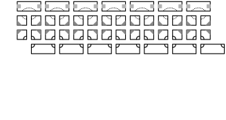
(b)

(c)

(d)

Fig. 3: The zig-zag tile set. (a) The width 4 zig-zag tile set and seed tiles. Each shape represents a single tile. Tiles have matching bonds of strength 1 when the shapes on their edges match. (b) The ribbon structure formed by the zig-zag tile set. (c) The L-shaped seed nucleates linear assemblies. (d) The W-shaped seed tile, with appropriate tiles for vertical zig-zag growth, could nucleate V-shaped assemblies.

(a)

(b)

Fig. 4: Zig-zag tile set growth. (a) Seeded growth of a zig-zag tile set in the aTAM. The same growth pattern occurs reversibly in the kTAM when $G_{mc}=2G_{se}-\epsilon$. (b) Unseeded growth. A possible series of steps by which the tiles could spuriously nucleate in the kTAM.

A self-assembly program is a set of tiles that assembles into a desired shape or set of shapes. The zig-zag tile set (Figure 3a of width $k$ contains tiles that assemble into a periodic ribbon of width $k$ (Figure 3b). Zig-zag tile sets of widths $k\geq 2$ can be constructed. A zig-zag tile set includes a top tile and a bottom tile, each having the same shape as 2 horizontally connected square tiles. Each of the $k-2$ rows between the top and bottom tiles contains two unique middle tiles that alternate horizontally. The alternation of two tile types along the columns enforces the column-wise staggering of the top and bottom tiles. Each tile label has exactly one match on another tile type, so the tiles cannot assemble to form any other structures held together by sticky end bonds.

The tile set is designed to operate in a physical regime where the attachment of a tile to another tile or assembly by two matching sides is energetically favorable, but an attachment by only one bond is energetically unfavorable. In the aTAM, these conditions translate to growth with a threshold of 2. Growth beginning from any non-seed tile in the zig-zag tile set goes nowhere in the aTAM—no two tiles can join by a bond with a strength of at least 2. In contrast, growth can proceed from an L-shaped or W-shaped seed tile (Figures 3c and 3d). Figure 4a illustrates the only possible growth path in the aTAM from the L-shaped seed. The staggering of the top and bottom tiles allows growth to continue indefinitely along a zig-zag path. Note that the top and bottom tiles alternately provide the only way to proceed to each successive column. Assemblies that do not span the full width ($k$ tiles) either cannot bind top tiles or cannot bind bottom tiles, and thus cannot grow indefinitely. Growth from a seed tile of less than full width would stall. For example, with a seed tile of width $k-1$, the top tile could not attach by two bonds to the assembly.

In the kTAM, seeded growth occurs in the same pattern as in the aTAM. Unlike in the aTAM, however, there are also series of reactions that can produce a full width assembly in the absence of a seed tile. The formation of such an assembly is called a spurious nucleation error. An example of such unseeded growth is shown in Figure 4b. Under the conditions of interest, some steps in spurious nucleation are energetically favorable, but at least $k-1$ must be unfavorable before the full-width assembly is formed. Once the full-width assembly is formed, further growth is favorable. Spurious nucleation is a transition from assembly melting, where assemblies are more likely to fall apart than they are to get larger, to assembly growth, where each assembly step is energetically favorable. Any assembly where melting and growth are both energetically favorable is called a critical nucleus.

Classical nucleation theory [56, 11] predicts that the rate of nucleation is limited by the concentration of the most stable critical nucleus, $[A_{c}]$. Intuitively, because more unfavorable reactions are required to form critical nuclei in a wider zig-zag tile set, $[A_{c}]$ should decrease exponentially with $k$. This argument is not rigorous, however, because the number of critical nuclei for a zig-zag tile set also increases with $k$. The rate of spurious nucleation is proportional to the sum of the concentrations of all these critical nuclei. We will show in the following sections that despite the increase in the number of kinds of critical nuclei that can form as $k$ increases, under many conditions nucleation rates do decrease exponentially with $k$.

3 The Self-Assembly Model

To analyze the process of tile assembly, we formally describe the mass-action kTAM. For a given tile set, kTAM describes the set of possible assemblies, their reactions and the dynamics of these reactions. The kTAM has been previously used to analyze complex tile programs [38, 47], and is a general framework for understanding algorithmic self-assembly. Here, we extend the kTAM to include polyomino tiles. We also introduce a variant of the kTAM in which the concentrations of all possible assemblies are considered. This is in contrast to the original kTAM, which tracks only a single, seeded assembly. Our extension is appropriate for studying nucleation, where growth can begin from any tile. Also in contrast to previous work with the kTAM, which used stochastic chemical kinetics, we introduce mass-action kinetics below. Both mass-action and stochastic kinetics are accepted models of chemical kinetics [12], but mass-action is more tractable analytically and the results of both models generally converge when a large populations of molecules are considered. In Section 6, we find that simulations of nucleation using stochastic kinetics are consistent with the bounds on nucleation rates we prove using the mass-action model.

A tile type $\mathbf{t}$ consists of a shape and a set of bond types on each unit edge of the shape. The shape is either a unit square or a polyomino, a finite, connected set of unit squares. The set of possible bond types is referred to as $\Sigma$. A set of tile types is denoted by $\mathbf{T}$. A tile (as contrasted with a tile type) is a tuple of a tile type and a location, which is specified by $L=(x,y)$, where $L$ is the coordinate location of the leftmost top unit square within the polyomino. The set of tiles (all possible tile types in all possible locations) is referred to as $\mathit{T}$. A translation of a tile has the same tile type as the original. Tiles cannot be rotated. Tiles that abut vertically or horizontally are bound if they have the same labels on the abutting sides. A set of tiles is bound if there is a path of bound tiles between any two tiles in the set.

An assembly $A$ is an equivalence class with respect to translation of a non-overlapping, bound finite set of one or more tiles. The set of assemblies is denoted by $\mathcal{A}$ and the set of assemblies consisting of two or more tiles is denoted $\mathcal{A}_{2+}$. We will also use the notation for the set of tiles, $T$ to refer to the assemblies that have only one tile, i.e. $\mathcal{A}-\mathcal{A}_{2+}$. A set of tiles $\tilde{A}$ is considered the canonical representation of $A$ if $\tilde{A}\in A$ and

$$\forall\langle\mathbf{t},(x_{i},y_{i})\rangle\in\tilde{A},x_{i}\geq 0\text{ and }y_{i}\geq 0\text{ and }$$

$$\exists y,\mathbf{t^{\prime}}\text{ s.t. }\langle\mathbf{t^{\prime}},(0,y)\rangle\in\tilde{A}\text{ and }$$

$$\exists x,\mathbf{t^{\prime\prime}}\text{ s.t. }\langle\mathbf{t^{\prime\prime}},(x,0)\rangle\in\tilde{A}$$

That is to say, the canonical representation uses a coordinate system such that the reference locations of the tiles just fit into in the upper right quadrant of the plane with no negative coordinates. Note that polyomino tiles may extend into the other three quadrants, so long as the location of the leftmost top unit of each polyomino is in the first quadrant. For an assembly $A$,

$$width(A)=\max_{x}|y_{1}-y_{2}|\;+\;1\text{, such that } \langle\mathbf{t_{1}},L_{1}\rangle,\langle\mathbf{t_{2}},L_{2}\rangle\in A,$$

$$(x,y_{1})=L_{1},(x,y_{2})=L_{2}.$$

This definition measures width with respect to the reference points for polyomino tiles, ignoring the extent of the other unit squares within the polyomino. $length(A)$, is defined analogously. Note that the definitions of $length$ and $width$ given here are designed to maximize the clarity of the analysis that follows, and may not be appropriate for other analyses of tile assembly. The addition relation is defined between an assembly $A\in\mathcal{A}_{2+}$ and a tile $t$ so that $A+t=B$ if and only if $\tilde{A}$ and $t$ are bound but non-overlapping, and $\tilde{A}\cup t$ is a member of equivalence class $B$. For the attachment of two tiles to each other, we need to be careful to correctly count the number of ways tiles can attach. We consider the set of tile types $\mathbf{T}$ to be listed in some order. The addition relation is defined between two tiles $t_{1}=\langle\mathbf{t_{1}},L_{1}\rangle$ and $t_{2}=\langle\mathbf{t_{2}},L_{2}\rangle$ if either $\mathbf{t_{1}}$ comes before $\mathbf{t_{2}}$ in the ordering of tiles or $\mathbf{t_{1}}=\mathbf{t_{2}}$ and for $L_{1}=(x_{1},y_{1})$ and $L_{2}=(x_{2},y_{2})$, either $y_{1}<y_{2}$ or $x_{1}<x_{2}$ and $y_{1}=y_{2}$ and $t_{1}\cup t_{2}=\tilde{A}$, for some $A\in\mathcal{A}$. In this case, $t_{1}+t_{2}=A$.

Bound tiles have a bond between them. The standard free energy, $G^{\circ}$, of an assembly $A$ is defined as $G^{\circ}(A)=-bG_{se}$, where $b$ is the number of bonds in the assembly and $G_{se}$ (the sticky end energy) is the unitless free energy of a single bond.

The dynamics in the kTAM consists of a set of reactions in which assemblies grow larger or smaller.

In this paper, we consider all possible accretion reactions: reactions either between two tiles or between a tile and an assembly. We also assume that the number of available single tiles does not change during the course of assembly (i.e. the reaction is “powered” by some process or circumstance that keeps monomer concentrations constant).

Formally, the set of powered accretion reactions are

$$R=\left\{A+t\rightarrow B+t,\;B\rightarrow A\;:\right.\ \left.A,B\in\mathcal{A}_{2+},\;\mathit{t}\in\mathit{T},\;A+\mathit{t}=B\right\}\;\cup\;\\ \left\{t_{1}+t_{2}\rightarrow A+t_{1}+t_{2},\;A\rightarrow\emptyset\;:\mathit{t_{1}},\mathit{t_{2}}\in\mathit{T},\;A\in\mathcal{A}_{2+},\;\mathit{t_{1}}+\mathit{t_{2}}=A\right\}$$

The appearance of single tiles on both sides of the association reactions and neither side of the dissociation reactions reflects the powered model’s assumptions that the number of single tiles remains constant.

In the mass-action kTAM, the dynamics of an assembly process are governed by mass-action kinetics. Mass-action kinetics is based on an ideal situation where tiles and assemblies exist in infinite quantities, and move at random through a solution of infinitely large volume. To distinguish the relative abundance of tile types and assemblies in the system, we use the notion of concentration, which denotes the number of copies of the relevant tile type or assembly within a unit volume. The concentration of species $A$ is denoted $[A]$.

Tiles and assemblies form or are consumed because of reactions that happen spontaneously or as a result of collisions between the reactants. This leads to the concentrations of assemblies changing over time. In a physical reaction vessel, an association reaction (a reaction where multiple species interact) occurs at a rate proportional to the frequency with which all the species involved come into physical contact. When the possible reactants are well-mixed and moving randomly through solution, the frequency with which such contact occurs is proportional to the product of the concentrations of all the reactant species. Likewise, dissociation reactions, which have only one reactant, occur randomly with constant probability per time unit per molecule. Even though individual reactions occur stochastically, when the number of particles is infinite, the total reaction rate is deterministic.

These observations lead to mass-action kinetics, which is an idealized model of chemical reactions in a well-mixed vessel [12]. The proportionality constant that relates the product of the concentrations of the reactant species to the rate at which the reaction occurs is a rate constant. In general, for a chemical reaction $\sum_{i}n_{i}S_{i}\rightarrow\sum_{j}m_{j}S_{j}$ with rate constant $k$, where $S_{i}$ are chemical species and $n_{i},m_{j}\in\mathds{Z}^{\geq 0}$ are the reactant and product stoichiometries (the number of times the reactant or product species occurs), mass-action dynamics [12] predict $\frac{d[S_{j}]}{ds}=k(m_{j}-n_{j})\prod_{i}[S_{i}]^{n_{i}}$. Mass action reactions occur in parallel, so that dynamics add linearly for multiple reactions.

In the kTAM, each reaction has a forward rate constant $k_{f}$ that we assume to be the same for all reactions, and a backward rate constant $k_{r}=k_{f}e^{-\Delta G^{\circ}}$, where $\Delta G^{\circ}$ is the difference between the sum of the unitless standard free energies of the reactants and that of the products (where the standard free energy of a single tile is 0). The concentration of all tile types is held at $e^{-G_{mc}}$. (Identical concentrations are considered for convenience only; Appendix A shows how our formalism can be extended trivially to treat reactions where species have different concentrations.) Assemblies consisting of more than a single tile have an initial concentration of 0. Thus, for an assembly $A$ at time point $s$,

$$\frac{d[A]}{ds}=k_{f}\biggl{(}\sum_{\begin{subarray}{c}A+\mathit{t}\rightarrow B+\mathit{t},\\ B\rightarrow A\;\in R\end{subarray}}e^{G^{\circ}(B)-G^{\circ}(A)}[B]-[A]e^{-G_{mc}}\;+\\ \sum_{\begin{subarray}{c}B+\mathit{t}\rightarrow A+\mathit{t},\\ A\rightarrow B\;\in R\end{subarray}}[B]e^{-G_{mc}}-e^{G^{\circ}(A)-G^{\circ}(B)}[A]\;+\sum_{\begin{subarray}{c}\mathit{t_{1}}+\mathit{t_{2}}\rightarrow A+\mathit{t_{1}}+\mathit{t_{2}},\\ A\rightarrow\emptyset\in R\end{subarray}}e^{-2G_{mc}}-e^{G^{\circ}(A)}[A]\biggr{)}.$$ (1)

Each term in the first summation is the difference between the rate at which $A$ and a tile react to form a larger assembly $B$ and the rate at which the larger assembly $B$ decomposes into $A$ and a tile. Each term in the second summation is the difference between the rate of formation of $A$ by a reaction where a single tile binds to a smaller assembly $B$, and the rate decomposition of $A$ into assembly $B$ and a single tile. The terms in the final summation are the rate of formation of $A$ from two single tiles and its dissociation into two single tiles. These final terms are nonzero only if $A$ is an assembly composed of exactly two tiles. In the remainder of this paper, we refer to the mass-action kTAM with powered accretion reactions as simply “the kTAM.”

The free energy $G(A)$, (in contrast to the standard free energy $G^{\circ}(A)$, reflects both the entropy loss due to crystal formation and the enthalpy gain of assembly. For an assembly $A$ with $n$ tiles and $b$ bonds, it is defined as $G(A)=G^{\circ}(A)+nG_{mc}$. The steady state concentration of an assembly $A$ is given by $[A]_{ss}=e^{-G(A)}=e^{\left(bG_{se}-nG_{mc}\right)}$. Recall that $G_{mc}>0$ and $G_{se}>0$, so that the energetic penalty of adding an additional tile can be compensated for by forming sufficiently many new bonds. A smaller $G(A)$ is more favorable, and corresponds to a higher steady state concentration.

This model satisfies detailed balance within $\mathcal{A}_{2+}$. That is, for all reaction pairs $A\rightarrow B$, and $A+t\rightarrow B+t$, $k_{f}[t][A]_{ss}=k_{r}[B]_{ss}$, where $k_{f}$ and $k_{r}$ are the forward and reverse rates in the respective reactions, and for reaction pairs $t_{1}+t_{2}\rightarrow A$ and $A\rightarrow\emptyset$, $k_{f}[t_{1}][t_{2}]=k_{r}[A]_{ss}$. A proof that the kTAM satisfies detailed balance is contained in Appendix A.

4 Thermodynamics of Zig-Zag Assemblies

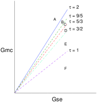
(a)

(b)

(c)

Fig. 5: Physical conditions where zig-zag polymer elongation is favorable. $G_{mc}$ (ln(tile concentration)) and $G_{se}$ (bond strength) define a set of physical conditions for zig-zag tile assembly. $\tau=\frac{G_{mc}}{G_{se}}$. (a) Phase diagram of the width 4 zig-zag tile set. In phase A, above the line $\tau=2$, no assembly reactions are favorable, whereas in regimes B,C,D,E and F, progressively more types of assemblies (shown in (b)) become favorable. (b) The polymeric assemblies which become favorable in the regimes B-F shown in (a). Polymers shown for earlier regimes are also favorable in later phases: the polymer shown for regime B is favorable in regimes C-F and so on. (c) The assemblies that can form from a zig-zag tile set of width $k$ and the physical conditions (in terms of $\tau$) in which these assemblies becomes favorable.

To prove that nucleation rates of zig-zag ribbons decrease exponentially as their widths increase, we would first like to identify the critical nuclei for spurious nucleation. Thermodynamic constraints provide a powerful tool: Because undesirable assemblies have unfavorable energies, we can conclude that they occur rarely without having to consider rates. (In contrast, assemblies with favorable energies may or may not form quickly, depending upon details of the kinetics; such analyses form the bulk of Sections 5 and 6.)

We therefore consider the free energy landscape, where each point in the landscape corresponds to a particular type of assembly. Optimal control over nucleation is achieved in a regime where zig-zag growth is favorable, but the growth of less than full-width (thin) assemblies is unfavorable.

Within the kTAM, the energy landscape for assemblies is formally described by the free energy $G(A)=nG_{mc}-bG_{se}$, which can be evaluated directly for any given assembly $A$. $G_{se}$ and $G_{mc}$ describe the physical conditions for assembly. Changing $G_{se}$ and $G_{mc}$ can bring the system into two qualitatively different phases. In the melted phase, $G(A)$ is bounded below by $G_{mc}$ for all $A$, meaning that no assembly has a concentration of more than $e^{-G_{mc}}$ at steady state. In contrast, in the crystalline phase, $G(A)$ can continue to decrease without bound (so $[A]_{ss}=e^{-G(A)}$ can increase without bound) as certain polymeric assemblies become longer and longer – that is, adding a repeat unit to the assembly strictly decreases its free energy. Within the crystalline phase, there are regimes where the elongation of different types of polymers are favorable or unfavorable. To ensure that thin polymers do not tend to grow, it is enough to show that for each of these polymer types, longer polymers have a higher free energy than shorter ones.

Fig. 6: Zig-zag polymerization reactions. The addition of a polymer unit to a thin assembly consists of an initial unfavorable accretion reaction followed by a series of favorable accretion reactions. (a) A favorable polymerization reaction. The positive free energy change from the four favorable accretion reactions is larger than the negative energy change from the initial unfavorable accretion reaction. Thus, the elongation of polymers of width 3 is favorable when $\tau=1.75$. (b) An unfavorable polymerization reaction. The positive free energy change from the two favorable accretion reactions is not large enough to compensate for the negative energy change from the initial unfavorable accretion reaction, so that the elongation of polymers of width 2 is unfavorable when $\tau=1.75$.

To characterize the energy landscape formally, we consider the important classes of polymeric assemblies and evaluate their free energies. Figure 5b, B-F show the 6 main types of polymeric assemblies for ribbons of width 4 by indicating the repeat group that may be added (by a series of accretion reactions, as shown in Figure 6) to extend the polymer. To determine whether adding a repeat group results in a higher or lower energy assembly, we evaluate $\Delta G=G(A_{m+1})-G(A_{m})=\Delta nG_{mc}-\Delta bG_{se}$ where $A_{m}$ is a polymeric assembly with $m$ repeat units. If $\Delta G$ is negative, then longer polymeric assemblies of this type are more favorable and we can expect this kind of assembly to grow at some rate. This gives a linear condition on $G_{se}$ and $G_{mc}$, specifying a regime of physical conditions in which a certain class of long assembly is favorable. For example, for polymer type E, each repeat unit adds 4 tiles ($\Delta n=4$) and 6 bonds ($\Delta b=6$) , so these polymers grow if $4G_{mc}-6G_{se}<0$, i.e. $\frac{G_{mc}}{G_{se}}<\frac{3}{2}$. Similar calculations result in the phase diagram shown in Figure 5a, which shows the melted phase A, in which no polymers are favorable, and the crystalline phase divided into regimes B-F wherein one additional type of polymer becomes favorable in each successive regime. In all these calculations, the ratio $\tau\stackrel{{\scriptstyle def}}{{=}}\frac{G_{mc}}{G_{se}}$ plays a critical role.

Figure 5c shows the $2k-3$ classes of polymeric assemblies for the width $k$ zig-zag tile set (excluding the full width ribbons) along with the condition on $\tau$ that determines when polymer elongation is favorable. Exclusively the elongation of full-width ribbons is favorable when $2>\tau>\frac{4(k-2)+1}{2(k-2)+1}=2-\frac{1}{2k-3}$. That is, when $2>\tau>2-\frac{1}{2k-3}$, zig-zag growth is favorable, but the elongation of all less than full-width polymers is unfavorable. The regime where $2>\tau>2-\frac{1}{2k-3}$ will be referred to as optimal nucleation control conditions.

Fig. 7: Reactions that increase width, the $\Delta G$ for those reactions, and the resulting conditions (in terms of $\tau$) where those reactions are favorable.

The table in Figure 7 enumerates the assemblies for which growing wider (rather than longer) is favorable. Like the polymerization of thin ribbons, a reaction to produce a wider assembly from a thinner one consists of an initial unfavorable accretion reaction followed by a series of favorable accretion reactions to complete the new row. The number of favorable reactions determines the values of $\tau$ for which the overall reaction is favorable. Very long but thin assemblies can favorably grow wider even when $\tau$ is close to 2, so for optimal nucleation control it is necessary that elongation of thin assemblies be unfavorable. Otherwise, a favorable path to nucleation exists: an assembly can grow longer until it is favorable for it to grow wider and then it can grow to full width.

An example of the difference in the energy landscape between the regime where only the elongation of full width polymers is favorable (optimal nucleation control conditions), and a regime where the growth of thinner polymers is also favorable can be seen in Figure 8. In each landscape, the critical nuclei divide the energy landscape into two basins whose lowest energy assemblies are infinite polymers or fully melted, respectively. A critical nucleus can, via a series of energetically favorable increases or decreases in length or width, either reach full width or melt away. The principal critical nucleus is the most stable critical nucleus. We start by considering the two landscapes under optimal nucleation control conditions, the two left landscapes of Figure 8. In these landscapes, the critical nuclei are of width $k-1$ (or width $k$) for both tile set widths and the most favorable path to nucleation for both tile sets is for a crystal of length 2 to grow to full width. Thus, the barrier to nucleation for a tile set of width 8 is higher than the barrier to nucleation for a tile set of width 4. In contrast, when $\tau=1.77$, the principal critical nucleus is the same for both tile sets: it is an assembly of width 3 and length 4. Under these conditions, the spurious nucleation rate of the tile set of width $k=8$ will not be appreciably smaller than nucleation rate of the tile set of width $k=4$.

Fig. 8: Example energy landscapes. Coarse-grained depictions of the energy landscapes for two zig-zag tile sets of different widths under two different physical conditions. Each square in the grid represents a “perfect” assembly of the labeled width and length. The shading in the square corresponding to each width and length represents the energy of a rectangular assembly of those dimensions. Darker is more favorable. Contour lines group assemblies of similar energies. Large circles denote assembly sizes that are critical nuclei. The most favorable critical nucleus (the principal critical nucleus) is denoted by a large hollow circle.

The primary theorem of the next section will apply only under optimal nucleation control conditions. While this region covers only a small fraction of area in the phase diagram shown in Figure 7, a slow anneal from a high temperature where $\tau\gg 2$ to a temperature in which $\tau<1$ will pass through this regime, and a slow enough anneal will allow the bulk of the reaction to take place in this regime. Therefore, it is reasonable to consider a mechanism for the control of nucleation which is valid only in this narrow range of physical conditions. In the next section, we analyze the nucleation rates of the zig-zag tile set within this regime.

5 An Asymptotic Bound on Spurious Nucleation Rates

The kinetic Tile Assembly Model predicts the concentration of each assembly at all times. For most tile sets, the number of possible assemblies is large, and the individual concentrations of many kinds of intermediate assemblies are not necessarily of interest. However, the sheer number of possible assemblies and possible assembly pathways can significantly affect the overall rate of spurious nucleation, and they can not simply be ignored. Understanding the contribution of many different assembly types to the total spurious nucleation rate is the main technical challenge in what follows. It is often helpful to talk about the concentration of a class $\mathcal{C}\subset\mathcal{A}$ of assemblies, $[\mathcal{C}]=\sum_{A\in\mathcal{C}}[A]$. The derivative of the concentration of a class of assemblies, $\frac{d[\mathcal{C}]}{ds}=\sum_{A\in\mathcal{C}}\frac{d[A]}{ds}$, can be calculated as the difference between the rate at which at which assemblies join the class and that at which they leave the class. Reactions which produce new members of the class from assemblies not in the class are the inward perimeter reactions, $R^{in}=\{A+t\rightarrow B+t,\;A\rightarrow B,\;t_{1}+t_{2}\rightarrow B+t_{1}+t_{2}:A\notin\mathcal{C},\;B\in\mathcal{C}\}$. Reactions which use up members of the class to produce assemblies not in the class (or single tiles) are the outward perimeter reactions = $R^{out}=\{B+t\rightarrow A+t,\;B\rightarrow A,\;B\rightarrow\emptyset:\;A\notin\mathcal{C},\;B\in\mathcal{C}\}$.

Define the flux across a set of reactions $R$ at time $s$ as

$$F(R,s)=\sum_{A+t\rightarrow B+t\in R}k_{f}[A]_{s}e^{-G_{mc}}+\sum_{B\rightarrow A\in R}k_{f}e^{G^{\circ}(B)-G^{\circ}(A)}[B]_{s}\;+\\ \sum_{t_{1}+t_{2}\rightarrow A+t_{1}+t_{2}\in R}k_{f}e^{-2G_{mc}}+\sum_{A\rightarrow\emptyset\in R}k_{f}e^{G^{\circ}(A)}[A]_{s}$$ (2)

where $[A]_{s}$ is the value of $[A]$ at time point $s$. Then $\frac{d[\mathcal{C}]}{ds}(s)=F(R^{in},s)-F(R^{out},s)$.

We will use these formalisms to bound the rate of spurious nucleation in a zig-zag tile set of width $k$. The spuriously nucleated assemblies for a zig-zag tile set of width $k$ will be denoted $\mathcal{C}_{k}$. Let the top tile in Figure 3(a) be designated $\mathbf{t_{t}}$, the bottom tile be $\mathbf{t_{b}}$, and the seed tile be designated $\mathbf{t_{s}}$. Formally,

$$\mathcal{C}_{k}=\{A\in\mathcal{A}:\;\exists(x,y),(w,z)\in\mathds{Z}^{2}\text{ s.t. }A(x,y)=\mathbf{t_{t}},A(w,z)=\mathbf{t_{b}},\;\text{ and }\\ \forall(q,r)\in\mathds{Z}^{2},\;\;A(q,r)\neq\mathbf{t_{s}}\}$$ (3)

Note that the assemblies in $\mathcal{C}_{k}$ do not contain a seed tile, and we are measuring the rate of formation of zig-zag ribbons without seed tiles.

(a)

(b)

(c)

Fig. 9: Spurious nucleation reactions. Three spurious nucleation reactions for a zig-zag tile set of width 4. The reaction may be either favorable or unfavorable. In (b), the addition is favorable when $G_{mc}=2G_{se}-\epsilon$ for small $\epsilon$, because two new bonds are formed; in (a) and (c), the addition is unfavorable, because in each reaction only one new bond is formed.

The inward perimeter reactions for $[\mathcal{C}_{k}]$, which we call the spurious nucleation reactions and denote by $R^{in}_{k}$, are the reactions for which the product is a full width assembly, but the reactant is not. In other words, they are the addition reactions which produce width $k$ assemblies from assemblies of width $k-1$ by adding either a top or bottom double tile (Figure 9). As shown in Section 4, under optimal nucleation control conditions these reactions demarcate the point at which sustained growth can proceed by exclusively favorable steps. The outward perimeter reactions, which we call the ribbon shrinking reactions and denote by $R^{out}_{k}$, are those in which a tile falls off a full width assembly to produce an assembly of width $k-1$. For assemblies that have suffered a ribbon shrinking reaction, there is also a downhill path to complete melting in an energy landscape of the type shown in Figure 8 under optimal nucleation control conditions.

The overall rate of spurious nucleation of width $k$ zig-zag crystals (in units of molar per second),

$$n_{k}(s)=\frac{d[\mathcal{C}_{k}]}{ds}(s)=F(R^{in}_{k},s)-F(R^{out}_{k},s),$$

may be integrated over time to obtain the total concentration of spuriously nucleated assemblies. Furthermore, an upper bound on $n_{k}(s)$ similarly translates into an upper bound on the concentration of spuriously nucleated assemblies. Because the growth path for full-width ribbons is so favorable (zig-zag growth), one such bound is obtained by neglecting the ribbon shrinking reactions and considering just the spurious nucleation reactions:

$$n^{+}_{k}(s)=F(R^{in}_{k},s)>n_{k}(s).$$

In what follows, “the rate of spurious nucleation” refers to $n_{k}(s)$, the rate at which the concentration of spuriously nucleated assemblies increases. We distinguish this rate from $n^{+}_{k}(s)$, the rate of formation of all full-width assemblies, whether they later shrink or not, by referring to the latter as “the rate of spurious nucleation reactions (or events).”

Theorem 1.

For a zig-zag tile set of width $k>2$, if $2>\frac{G_{mc}}{G_{se}}>2-\delta$, $\delta<\frac{1}{2k-3}$, and $G_{se}>\frac{2k\ln{2}}{1-(2k-3)\delta}$, then for all times $s$, $n_{k}(s)<4k_{f}e^{(\delta-k)G_{se}}$.

Proof.

Since $n_{k}^{+}(s)<n_{k}(s)$, we can prove the theorem by showing that $n_{k}^{+}(s)<4k_{f}e^{(\delta-k)G_{se}}$. All the spurious nucleation reactions are addition reactions, so if we compute $n_{k}^{+}(s)$ using Equation 2, the second and fourth terms of the expression are both zero. Spuriously nucleated assemblies are defined as assemblies of width $k$, so the reactants in the spurious nucleation reactions are of width $k-1$ (only accretion reactions are allowed). For a tile set of width $k>2$, the third term of Equation 2—the contribution of the interaction of two tiles—also drops out. Therefore, for a tile set of width $k>2$ with spurious nucleation reactions $R^{in}_{k}$,

$$n_{k}(s)\leq n^{+}_{k}(s)=\sum_{A+\mathit{t}\rightarrow B+\mathit{t}\in R^{in}_{k}}k_{f}[A]e^{-G_{mc}},$$ (4)

where $[A]$ is the concentration of assembly $A$ at time point $s$.

While it is in general difficult to calculate $[A]$ at an arbitrary time point, the following lemma shows that the concentration of an assembly can be bounded by its concentration at steady state, which is easy to compute:

Lemma 2.

In a mass-action powered accretion kTAM, if in the initial state only single tiles have a positive concentration, then every assembly has a concentration less than or equal to its steady state concentration at all time points.

Proof.

See Appendix B. ∎

Lemma 2 implies that

$$F(R^{in}_{k},s)\leq\sum_{A+\mathit{t}\rightarrow B+\mathit{t}\in R^{in}_{k}}k_{f}[A]_{ss}e^{-G_{mc}}$$

where $[A]_{ss}$ is the concentration of assembly $A$ at steady state.

Partitioning the summation according to the length of the reactant assembly gives

$$F(R^{in}_{k},s)\leq\sum_{l=1}^{\infty}\sum_{\begin{subarray}{c}length(A)=l\\ A+t\rightarrow B+\mathit{t}\in R^{in}_{k}\end{subarray}}k_{f}[A]_{ss}e^{-G_{mc}}.$$ (5)

  

(a)

(b)

Fig. 10: Assembly dimensions of rectangular assemblies. (a) A $k-1=3$ by $l=8$ assembly. (b) A $k-1=3$ by $l=7$ assembly.

To be a reactant in a spurious nucleation reaction, $A$ must have a width of $k-1$. Because all bonds in an zig-zag tile set assembly are unique to a given location within the ribbon repeat unit, any potential tile addition either matches the assembly on all sides, such that no errors occur, or matches on no sides, such that the addition does not produce a bound assembly. Thus, $A$ cannot have any mismatches. Each assembly $A$ in the preceding summation can therefore be viewed as a $k-1$ by $l$ rectangular assembly of one of the types shown in Figure 10 with zero or more tiles missing. $2G_{se}>G_{mc}$ by assumption, so the free energy of a $k-1$ by $l$ assembly cannot be more favorable than the free energy of the $k-1$ by $l$ rectangle that contains it, since any missing tiles in the rectangle could be added by favorable reactions. Therefore, the concentration of any $k-1$ by $l$ assembly at steady state must be no larger than the concentration of its corresponding $k-1$ by $l$ rectangular assembly. Note that this bound is very loose, since most assembly types have several tiles attached by only one bond and therefore have a higher free energy. Let $A_{k-1,l}$ be a $k-1$ by $l$ rectangular assembly, and $C(k-1,l)$ be the number of assemblies of width $k-1$ and length $l$. Each assembly can bind a single tile in up to $l/2$ locations (since the tile must be a double tile) along either the top or bottom edge. Thus,

$$F(R^{in}_{k},s) <\sum_{l=1}^{\infty}\sum_{\begin{subarray}{c}length(A)=l\\ A+t\rightarrow B+\mathit{t}\in R^{in}_{k}\end{subarray}}k_{f}[A_{k-1,l}]_{ss}e^{-G_{mc}}$$ (6)

$$\leq\sum_{l=1}^{\infty}C(k-1,l)\frac{l}{2}k_{f}[A_{k-1,l}]_{ss}e^{-G_{mc}}.$$ (7)

A counting argument shows that $C(k-1,l)<2^{(k-1)l+1}$, so

$$F(R^{in}_{k},s)<\sum_{l=1}^{\infty}2^{(k-1)l}lk_{f}[A_{k-1,l}]_{ss}e^{-G_{mc}}.$$ (8)

The steady state concentration of an unseeded assembly with $n$ tiles and $b$ bonds is given by $[A]_{ss}=e^{-nG_{mc}+bG_{se}}$. The assembly $A_{k-1,l}$ contains $(k-2)l$ small tiles and $\lceil l/2\rceil$ top (or bottom) tiles. There are $(l-1)(k-2)$ horizontal bonds between small tiles and $\lceil l/2\rceil-1$ horizontal bonds between large tiles. In addition, there are up to $l$ vertical bonds in each of the $k-2$ spaces between rows of tiles. Therefore,

$$[A_{k-1,l}]_{ss}\leq\exp\left(-\left((k-2)l+l/2\right)G_{mc}\;+\right.\left.\left((k-2)(l-1)+l/2+(k-2)l\right)G_{se}\right).$$

Applying the assumption $G_{mc}>(2-\delta)G_{se}$ and simplifying,

$$[A_{k-1,l}]_{ss}< \exp\left[(2-k)G_{se}+(k\delta-\frac{1}{2}-\frac{3\delta}{2})lG_{se}\right].$$

Thus,

$$F(R^{in}_{k},s)<\;k_{f}e^{-G_{mc}}e^{(2-k)G_{se}}\sum_{l=1}^{\infty}l2^{(k-1)l}e^{(k\delta-\frac{1}{2}-\frac{3\delta}{2})lG_{se}}$$

Since $k\delta-\frac{1}{2}-\frac{3\delta}{2}<0$ when $k>2$ and $\delta<\frac{1}{2k-3}$, bounding $G_{se}$ from below preserves the inequality. Therefore, when $G_{se}>\frac{2k\ln(2)}{1-(2k-3)\delta}$,

$$F(R^{in}_{k},s)< \;k_{f}e^{-G_{mc}}e^{(2-k)G_{se}}\sum_{l=1}^{\infty}l2^{(k-1)l}e^{(k\delta-\frac{1}{2}-\frac{3\delta}{2})l\frac{2k\ln(2)}{1-(2k-3)\delta}}$$ (9)

$$= \;k_{f}e^{-G_{mc}}e^{(2-k)G_{se}}\sum_{l=1}^{\infty}l2^{(k-1)l}e^{-kl\ln{2}}$$ (10)

$$= \;k_{f}e^{-G_{mc}}e^{(2-k)G_{se}}\sum_{l=1}^{\infty}l2^{-l}$$ (11)

$$= \;2k_{f}e^{-G_{mc}}e^{(2-k)G_{se}}$$ (12)

$$= \;2k_{f}e^{(\delta-k)G_{se}}.$$ (13)

∎

This theorem says that the spurious nucleation rate, $n_{k}$, decreases exponentially with $k$ and with $G_{se}$, within the limits of applicability of the theorem—which requires larger $G_{mc}$ for larger $k$, and hence slower growth rates. The strength of the theorem, therefore, lies in the extent to which spurious nucleation decreases faster than the growth rate, $r_{k}$, of seeded crystals. These relative rates translate into the degree of purity that can be obtained when attempting to grow seeded crystals: suppose the concentration of seeds is $c$, and they are grown to a length $L$ during a time period $s=L/r_{k}$. The concentration of unseeded crystals that will have spuriously nucleated in that time is less than $s\cdot n_{k}=L\cdot\frac{n_{k}}{r_{k}}$, i.e., the fraction of crystals that were spuriously nucleated is less than $\frac{L}{c}\cdot\frac{n_{k}}{r_{k}}$. (When we use $n_{k}$ without specifying a particular time, we mean its steady state value, which is an upper bound.) Regardless of what length or amount of seeded crystals is desired, reducing $\frac{n_{k}}{r_{k}}$ is the relevant metric for increasing the yield of desired structures.

One way to study the trade-off between $n_{k}$ and $r_{k}$ is to ask, given a target growth rate $r$, what is the lowest nucleation rate that can be achieved by adjusting $G_{mc}$ and $G_{se}$ while maintaining $r_{k}=r$? Previous work [51] has shown that near the $\tau=2$ phase boundary that is relevant to our theorem, the growth rate is closely approximated by

$$r_{k}=\frac{k_{f}}{k-1}(e^{-G_{mc}}-e^{-2G_{se}})$$

measured in layers per second. The lowest nucleation rate for a given target growth rate $r$ is then $n^{*}_{k}(r)=\min_{\begin{subarray}{c}G_{se},G_{mc}\\ \hbox{\ s.t.\ }r_{k}=r\end{subarray}}n_{k}$. A plot of $n^{*}_{k}(r)$ vs $r$, if it could be calculated, would reveal how much the spurious nucleation rate decreases when the growth rate is decreased. Theorem 1 only gives us an upper bound on $n^{*}_{k}(r)$, but even so, this already gives us a characterization of the advantage provided by wider zig-zag crystals.

Specifically, choosing $2G_{se}-G_{mc}=\epsilon=\ln k$, $\delta=\frac{1}{2}\left(\frac{1}{2k-3}\right)$ and $G_{se}>4k\ln k$, then Equation 13 guarantees that

$$n^{*}_{k}<n_{k} <2k_{f}e^{-G_{mc}}e^{(2-k)G_{se}}$$

$$=2k_{f}e^{-(G_{mc}-2G_{se})}e^{-kG_{se}}$$

$$=2k_{f}e^{\epsilon}e^{-kG_{se}}$$

$$=2k_{f}e^{\ln{k}}e^{-kG_{se}}$$

$$=2k_{f}ke^{-kG_{se}}.$$

Define $n^{B}_{k}=2k_{f}ke^{-kG_{se}}$. Also

$$r_{k}=\frac{k_{f}}{k-1}(e^{-G_{mc}}-e^{-2G_{se}})=\frac{k_{f}}{k-1}(e^{\epsilon-2G_{se}}-e^{-2G_{se}})=k_{f}e^{-2G_{se}}.$$

The ratio $\frac{n_{k}}{r_{k}}$ describes the trade-off between assembly speed $r_{k}$ and spurious nucleation $n_{k}$. This ratio can be no larger than $\frac{n^{B}_{k}}{r_{k}}$. For $k>2$ and the chosen parameters,

$$\frac{n^{B}_{k}}{r_{k}}=\frac{2k_{f}ke^{-kG_{se}}}{k_{f}e^{-2G_{se}}}=2ke^{(2-k)G_{se}}<2ke^{(2-k)4k\ln{k}}.$$

which decreases exponentially with $k$. Thus, under these conditions, seeded zig-zag crystals can be grown with exponentially greater yield as width increases.

The bound $n^{B}_{k}$ where $\epsilon=0.1$ is plotted against $r_{k}$ in Figure 11 for $k=3,\;4,\;5$ and $6$. While these bounds characterizing the trade off between $n^{*}_{k}$ and $r_{k}$ are rigorous, because Theorem 1 is so loose, it is expected that $n^{*}_{k}$ is actually much lower than the bound $n^{B}_{k}$. In the following sections, we will see that this is true; furthermore, the true slopes are even steeper than obtained by Theorem 1.

6 Numerical Estimates of Spurious Nucleation Rates

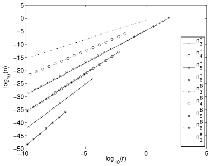
Fig. 11: Analytical upper bounds, steady-state calculations and asymptotic simulations of spurious nucleation rates. The graph compares the growth rate $r_{k}$ (in layers/s) and the rate of spurious nucleation events, $n^{+}_{k}$ (in M/s), for $2G_{se}-G_{mc}=\epsilon=0.1$. $k_{f}=6\times 10^{5}/M/s$ and for all points $G_{se}>\frac{2k\ln{2}}{1-(2k-3)\delta}$ for $k=3,4,5$ and $6$. Analytical upper bounds on the nucleation rate ($n^{B}_{k}=4k_{f}e^{(\delta-k)G_{se}}$) are those given by Theorem 1. The method of numerical calculation of spurious nucleation reaction rates at steady state, $n^{+}_{k}$, is described in Section 6.1. Stochastic simulation methods (giving $n^{\#}_{k}$) are described in Section 6.2.

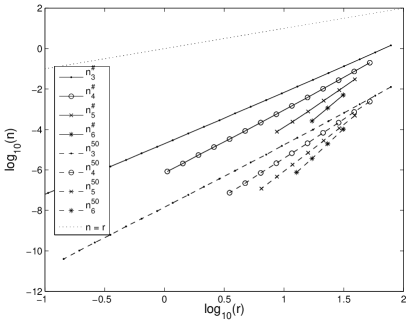
Fig. 12: Estimates of nucleation rates from stochastic simulations. $n^{\#}_{k}$ and $n^{50}_{k}$ vs. $r_{k}$ for $k=3,\;4,\;5$ and $6$. $\epsilon=0.1$. The line $n=r$ is also plotted to illustrate values of $n$ if there were no improvement in nucleation rates with assembly slowdown.

Having proven in the previous section that zig-zag tile sets can be designed to achieve arbitrarily low spurious nucleation rates relative to the growth rates (using a loose upper bound), we now ask whether the nucleation barrier provided by zig-zag tile sets is sufficient for practical implementation in the laboratory (which requires more accurate quantitative assessments). There are two main concerns: first, as each tile must be synthesized, $k$ must be small (6 is currently practical, while 50 is currently too large); second, assembly time must not be too long. (Growing 1000 layers of seeded crystals with less than 1% spurious nucleation—which we refer to as the “typical reaction”—seems like a reasonable goal to accomplish within one week.) Because the analytic bounds of Section 5 are too loose to allow us to obtain a realistic evaluation of nucleation rates, we now develop more accurate numerical calculations and stochastic simulations for estimating spurious nucleation rates.

The analysis in Section 5 overestimates the spurious nucleation rate in three ways. First, it overestimates the concentration of almost all kinds of assemblies by assuming they have the same concentration as a rectangular assembly of the same length and width, and it overcounts the number of different types of assemblies. Second, Lemma 2 shows that the spurious nucleation rate at steady state is the maximal spurious nucleation rate. However, it may take longer to approach steady state than the time needed to run a “typical reaction,” and far from steady state, the spurious nucleation rate may be much smaller than the spurious nucleation rate at steady state. Lastly, this analysis defines a spurious nucleation event for a zig-zag tile set of width $k$ as a reaction that produces an assembly of width $k$, and neglects the backward reaction. In practice, many reactions that form an assembly of width $k$ are unfavorable, so that the product assembly frequently shrinks back to a sub-critical size instead of growing larger. When conditions only slightly favor growth, even assemblies containing several layers have a reasonable chance of shrinking to nothing before they grow substantially. We expect $n_{k}<<n^{+}_{k}$ in this case.

While it is not possible to compute the nucleation rate exactly, in this section we describe three numerical techniques that correct each inaccuracy described above for zig-zag tile sets of widths $k=3,\;4,\;5$ and $6$. In Section 6.1, we compute the rate at which ribbons of width $k$ are formed at steady state using a much more accurate count of the number and steady state concentration of assemblies.. These computations show that the analytic bound of Theorem 1 is too high by at least 4 orders of magnitude for the range of parameters studied. In Section 6.2 we use a stochastic simulation of tile assembly to estimate the rate of spurious nucleation reactions $R^{in}_{k}$. Our results indicate that spurious nucleation reactions occur during a “typical reaction” at a rate that is no more than an order of magnitude lower than the rate at steady state computed in Section 6.1. In Section 6.3, we use the stochastic simulation to investigate whether the rate of spurious nucleation reactions ($n^{+}_{k}=F(R^{in}_{k},s)$) in a typical reaction accurately predicts the rate at which large assemblies appear (which at steady state is equivalent to $n_{k}(s)=F(R^{in}_{k},s)-F(R^{out},s)$). We find that for the range of parameters studied, at least 99% of assemblies that reach full width will melt before growing into large crystals, and thus our other estimates of spurious nucleation rates may be overestimates of $n_{k}$ by at least two orders of magnitude. In Section 6.4, we show that these results together indicate that a zig-zag tile set of width 5 or 6 should be large enough to prevent almost all spurious nucleation in a “typical reaction”, while maintaining reasonable assembly speeds. We conclude with an important caveat to these results. Our results are derived under a powered accretion model of kTAM, while in experiments, small assemblies may aggregate rather than growing exclusively by single tile additions, thus potentially producing nuclei that reach a critical size more quickly than our simulations indicate.

6.1 Spurious Nucleation Rates at Steady State

Recall that for a zig-zag tile set of width $k>2$, the steady state rate of spurious nucleation reactions is given by the sum

$$n^{+}_{k}=\lim_{s\rightarrow\infty}F(R^{in}_{k},s)=\sum_{l=1}^{\infty}\ \ \ \sum_{\begin{subarray}{c}A+t\rightarrow B+\mathit{t}\in R^{in}_{k}\\ \text{s.t. }length(A)=l\end{subarray}}k_{f}[A]_{ss}e^{-G_{mc}},$$

which ignores the rate at which spuriously nucleated assemblies dissolve back into pre-nucleated assemblies. While $[A]_{ss}$ is known (at steady state, for an assembly $A$ with $n$ tiles and $b$ bonds, $[A]_{ss}=e^{bG_{se}-nG_{mc}}$), it is not practical to compute the sum exactly because there are an infinite number of spurious nucleation reactions. Additionally, it can be impractical to evaluate the inner sum even for a single value of $l$: no efficient algorithm is known for exactly enumerating the reactions in $R^{in}_{k}$ (see e.g. [19] for the related problem of counting polyominos). The number of distinct reactions increases exponentially with the length of $A$, so it is prohibitive to calculate all but the first terms of the sum.

Despite these difficulties, the expression can be calculated precisely, with known error bounds, for many $k$. The following lemma shows that under many reaction conditions of interest, the sum converges quickly, and its value can be approximated by summing only the first few terms:

Lemma 3.

When $G_{se}>(\ln 10)(k-2)+\ln{4}$, $G_{mc}=\>2G_{se}-\epsilon$, $0\leq\epsilon<\frac{1}{2k-3}$ $,k>2$ and $l$ is even,

$$\sum_{p=l+1}^{\infty}\left(\sum_{\begin{subarray}{c}A+t\rightarrow B+\mathit{t}\in R^{in}_{k}\\ \text{s.t. }length(A)=p\end{subarray}}k_{f}[A]_{ss}e^{-G_{mc}}\right)<2\left(\sum_{\begin{subarray}{c}A+t\rightarrow B+\mathit{t}\in R^{in}_{k}\\ \text{s.t. }length(A)=l\end{subarray}}k_{f}[A]_{ss}e^{-G_{mc}}\right)$$

Proof.

See Appendix C. ∎

Thus, to calculate the spurious nucleation rate up an accuracy of $\frac{1}{\varepsilon}$, it is only necessary to compute the inner sums of the series until the sum the current value of $l$ is (even and) less than $\frac{1}{2\varepsilon}$. (Note that this approach does not directly yield a proof of an analytic bound for arbitrary $k$, because the formula for the nucleation rate is not a closed form expression.)

We have used this series truncation method to calculate the rate of spurious nucleation to 1 part in $10^{4}$ for $k=3,\;4,\;5$ and 6 and for a range of $G_{se}$, $G_{mc}$ for which $\epsilon=0.1$. The values of $G_{se}$, $G_{mc}$ and $k$ used were in a regime in which Lemma 3 applies. The results are shown in Figure 11.

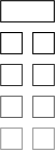
Fig. 13: Hypothesized principal critical nucleus for most spurious nucleation reactions. The rate of spurious nucleation reactions by this assembly (shown in successively lighter shades of gray for tile sets of widths $3,\;4,\;5$ and 6) accounts for a large portion of spurious nucleation at slow speeds, and also accounts for the rate of increase in spurious nucleation rates as assembly gets faster.

In addition to the numerical calculations providing lower estimates, the slopes of $\log n^{+}_{k}$ vs $\log r_{k}$ in Figure 11 are larger than those of $\log n^{B}_{k}$ vs $\log r_{k}$. Specifically the numerical calculations give slopes $\frac{k+2}{2}$, compared to the analytic bounds that give slopes $\frac{k}{2}$. Is this reasonable? In the limit as $G_{mc}\rightarrow\infty$, all spurious nucleation should be dominated by the single species with the highest steady state concentration (adding tiles become so unfavorable that other species can be neglected.) The analysis in Section 4 suggests that this assembly is the one shown in Figure 13. The steady state concentration of this assembly $A$ for a tile set of width $k$ is $[A]_{ss}=e^{-(2k-3)G_{mc}+(3k-6)G_{se}}=e^{-kG_{se}+(2k-3)\epsilon}$, where $\epsilon=2G_{se}-G_{mc}$. If all forward nucleation reactions involve $A$, then

$$n^{+}_{k}\approx 2k_{f}[A]_{ss}e^{-G_{mc}}=2k_{f}e^{-(k+2)G_{se}+(2k-4)\epsilon}$$ (15)

while the speed of growth is

$$r_{k}=\frac{k_{f}}{k-1}\left(e^{-G_{mc}}-e^{-2G_{se}}\right)=k_{f}e^{-2G_{se}}\frac{e^{\epsilon}-1}{k-1},$$

and thus the slope would be $\frac{k+2}{2}$, as observed. The rough estimate of $n^{+}_{k}$ given in Equation 15 is within a factor of three of the value calculated to an accuracy of 1 part in $10^{4}$, as guaranteed by Lemma 3.

6.2 Stochastic simulations for estimating forward nucleation rates before steady state is achieved

Tile set width	$n^{+}_{k}$	$n^{\#}_{k}$	$n^{50}_{k}$
3	$3\times 10^{24}$ years	$1\times 10^{23}$ years	$9\times 10^{5}$ years
4	$2\times 10^{8}$ years	$3\times 10^{6}$ years	$7$ years
5	900 years	$10$ years	$20$ days
6	2 years	$20$ days	$20$ hours

Table 1: Estimated time needed to grow 1000 layers in 1 pmol of free tiles without any spurious nucleation, based on approximations of the spurious nucleation rate. While the total number of tiles in each reaction is constant, the volume differs depending on the speed, which determines the concentration and the spurious nucleation rate.

Tile set width	$n^{+}_{k}$	$n^{\#}_{k}$	$n^{50}_{k}$
3	$1\times 10^{11}$ years	$1\times 10^{10}$ years	200 days
4	40 years	5 years	12 hours
5	10 days	2 days	1 hour
6	7 hours	2 hours	15 minutes

Table 2: Estimated time needed to grow 1000 layers such that less than 1 percent of assemblies are spuriously nucleated based on approximations of the spurious nucleation rate. The seed concentration is $\frac{1}{1000}$ the concentration of free tiles $e^{-G_{mc}}$.

In order to determine whether the steady state approximation is accurate over a typical spurious nucleation reaction, we simulated zig-zag tile assembly for tile sets of widths $k=3,\;4,\;5$ and $6$ and measured the rates of spurious nucleation events during the time it should take to grow 1000 layers from seeds. Since there are an infinite number of powered accretion reactions, exact simulation of growth under the kTAM using mass action dynamics is not possible. Instead, we simulated assembly growth using stochastic chemical reaction dynamics for discrete numbers of molecular assemblies. Here, simulation is possible because even though the probability of any of the infinite number of species arising is larger than 0, the total number species tracked at a given time is finite. To approximate the nucleation rate, we simulated a tiny reaction volume, and used these results to predict the nucleation rate in a much larger volume.

We used the Gillespie algorithm [18] to sample the trajectories of stochastic dynamics of the zig-zag tiles in a small volume $V$, whose value is chosen to ensure the accuracy of our nucleation rate estimate as described below. Following the powered model, our simulation assumes the concentration of each tile type to be constant and explicitly tracks each assembly in the volume containing more than one tile. Initially, no multi-tile assemblies are present. Single tiles are present at a concentration of $e^{-G_{mc}}$, so the rate of two tiles colliding (and thus producing a new assembly to be explicitly tracked) is $\mathbf{A}k_{f}Ve^{-2G_{mc}}$ molecules / second where $\mathbf{A}$ is Avogadro’s number. For each assembly containing two or more tiles, the rate of tile addition at each available site is $k_{f}e^{-G_{mc}}$ and the rate at which a tile with $b$ bonds falls off an assembly is $k_{f}e^{-bG_{se}}$.

For $k=3,\;4,\;5$ and $6$ and a range of $G_{se}$ and $G_{mc}$ where $\epsilon=0.1$, we counted the number of spurious nucleation events, $m$, that took place over the time course of a “typical reaction”, $s=1000/r_{k}$, in a volume $V$ that was chosen large enough to ensure that statistical error in $m$ is less than 10 percent of its value ($P>0.95$). If our simulations yield a nucleation rate of $m$ events per second, the molar rate of nucleation events for a bulk volume is given by $n^{\#}_{k}\approx\frac{m}{V\mathbf{A}}$. The results of the simulation—which were possible only for small enough $G_{se}$ such that nucleation events were frequent enough to be counted—are shown in Figure 12. For $k=3$ and $k=4$, these rates are within a factor of 2 of the linear extrapolation of the curves from Figure 11, and for $k=5$ and $k=6$ these rates are within a factor of 10, indicating that the choice in Section 5 to bound nucleation rates based on steady state concentrations did not affect our estimate of nucleation rates too greatly. This should be expected, given that under the conditions we studied most steady state nucleation appears to involve assemblies like the one shown in Figure 13.

6.3 Nucleation of Long Ribbons

In this paper, we have defined a spurious nucleation reaction for a zig-zag tile set of width $k$ as a reaction in which an assembly of width $k-1$ grows to width $k$. The goal was that this definition would be inclusive, such that all long ribbons would undergo at least one spurious nucleation reaction, but not too loose, such that most spurious nucleation reactions lead to a long ribbon. However, many of these spurious nucleation reactions are not energetically favorable—an assembly may briefly reach width $k$ before a tile falls off. The assembly then either melts or undergoes another spurious nucleation reaction.

At what rate do long ribbons appear? Using the stochastic simulation described in the last section and the same range of physical reaction parameters, we measured $m^{\prime}$, the number of ribbons containing 50 tiles or more that were present at the end of a “typical reaction”, for the widths 3, 4, 5, or 6. $m^{\prime}$ is an estimate of the number of spurious nucleation events that did not subsequently melt, and thus it provides the basis for an estimate for $n_{k}$. As only those crystals that nucleated sufficiently far before the end of the simulation will have grown to a large enough size to have been counted, we use the formula $n^{50}_{k}\stackrel{{\scriptstyle def}}{{=}}\frac{m^{\prime}}{(s-\left(50r_{k}/(k-1)\right))V\mathbf{A}}$, where $s$ is the time of the simulation and $50r_{k}/(k-1)$ is the approximate time to grow to 50 tiles via zig-zag growth. The results are shown in Figure 12.

These simulations suggest that much of the looseness of the analytical bound on nucleation, $n^{B}_{k}$, is caused by our neglecting crystals which under go a nucleation reaction and subsequently melt. These simulations suggest that at least 99% of crystals that undergo a spurious nucleation do not grow into crystals consisting of 50 or more tiles. That is, $n_{k}\ll n^{+}_{k}$.

6.4 Expected Effectiveness in Practice

Do these results indicate that nucleation control with tile sets of width 6 or less are good enough? Recall that our “reasonable goal for a typical reaction” addresses how much time is needed to grow seeded ribbons of 1000 layers with less than 1% of the crystals being spuriously nucleated. The fraction of crystals that are spuriously nucleated is given by $f=\frac{L}{c}\frac{n_{k}}{r_{k}}$, where $L$ is the number of layers to be grown on seeds, and $c$ is the concentration of seeds. While the simulations only measured $n_{k}$ for large values of $r_{k}$, it is possible to approximate $n_{k}$ for smaller values of $r_{k}$ by assuming that the graph of $\log(n_{k})$ vs. $\log(r_{k})$ continues as a line with constant slope as $r_{k}$ and $n_{k}$ decrease. We consider two cases. The first situation (more stringent than “reasonable”) is to grow many ribbons — say, from 1 picomole of each tile type, making $6\times 10^{8}$ ribbons of length 1000 — and not have more than a single spuriously nucleated crystal, i.e., $f<1.67\times 10^{-9}$ and $c=e^{-G_{mc}}/1000$. To satisfy this constraint, we express $f$ in terms of $c$ using our estimates for $n_{k}$, and solve for $c$ (and hence the concentration of free tiles and the volume of the reaction by $\mathbf{A}e^{-G_{mc}}V=10^{-12}$ moles). The time needed to grow the crystals is therefore given as $L/r_{k}$ for these conditions. The results, shown in Table 1, suggest that if $n^{50}_{k}$ is accurate, then this stringent goal could be met using a width 6 zig-zag tile set and a day of growth. The looser estimates and smaller tile set widths are less encouraging. The second situation we consider is the “reasonable” one; again, $c=e^{-G_{mc}}/1000$, but now we only require $f<0.01$. The results are shown in Table 2. In this case, acceptable growth fidelity is predicted to be achieved in less than an hour for width 6, and for only slightly longer times for widths 5 and 4. However, all these estimates are very sensitive to the coefficients of the linear fits to $\log{n_{k}}$ vs $\log{r_{k}}$, which are imperfect because the relationship is not perfectly linear.

The analysis and simulations in this section support the idea that nucleation control using the zig-zag tile set not only works in theory, but should be practical. While in most respects our models appear complete, two effects which may be important in the actual process of assembly are not included. One such effect is tile depletion: while our model considers the concentration of free tiles to be constant, in a typical experiment tiles are used up because they join assemblies. Since the rate of spurious nucleation is concentration dependent, we would expect the rate of spurious nucleation to be larger at the beginning of a reaction, when almost all free tiles remain, than at the end, when many tiles are used up. Because of this effect, our simulations may actually overestimate the spurious nucleation rate in experimental systems.

However, our simulations also neglect an important possible reaction pathway that may greatly increase the rate of spurious nucleation. While our model assumes tiles must be added to assemblies one at a time, in an experiment, small assemblies can also attach to each other. The formation and joining of several small assemblies may be faster than the spurious nucleation pathways described in this paper. A complete understanding of spurious nucleation of zig-zag tiles requires an understanding of the speed of spurious nucleation reactions caused by the joining of small assemblies.

7 Conclusions

7.1 Nucleation of Algorithmic Self-Assembly

Our original motivation was to show that self-assembly programs that work in the aTAM, in which it is straightforward to design tile sets that algorithmically assemble any computationally defined structure, can also be made to work in the more realistic kTAM.

While tile sets that assemble correctly via unseeded growth in the aTAM with a threshold of $\tau=1$ will assemble correctly in the kTAM under the right conditions, programs to assemble structures can be exponentially larger (in terms of number of tile types) than those with a threshold of $\tau=2$ [38]. However, tile sets that are designed to assemble via seeded growth in the aTAM with a threshold $\tau=2$ may fail in the kTAM because mismatch, facet and spurious nucleation errors occur. These problems are ameliorated in the limit of slow assembly speed [51]. Other work has described methods to control mismatch errors and facet errors without significant slowdown [52, 7, 34]. Here, we have developed a construction that may be used to correct the last discrepancy, spurious nucleation errors, again without significant slowdown.

It remains to be formally proven that these constructions can be combined to control all types of errors simultaneously for any tile set of interest. No major difficulties are expected, however, in large part because mismatch and facet errors can both be controlled by a single mechanism [7] and the control of spurious nucleation errors works independently of this mechanism. Both methods work by transforming an original tile set which works in the aTAM at $\tau=2$ into a new (typically larger) tile set that is more robust to particular kinds of errors in the kTAM.

After this paper was submitted, experimental demonstration of a decrease in nucleation rates with ribbon width have supported the predictions made here [42]. Further experiments combining the techniques described here with proofreading techniques, as predicted, resulted in algorithmic assembly where both mismatch error rates and spurious nucleation error rates are low [4], and has enabled other algoithmic self-assembly experiments [16]. It remains to be seen whether facet nucleation rates can be lowered in experimental demonstrations of algorithmic self-assembly, but the principal mechanism in the theoretical proposal for lowering facet nucleation error rates [7] has been has been experimentally confirmed [8].

7.2 Detection of a Single DNA Molecule

Fig. 14: Exponential amplification of assemblies. Probe strands assemble onto a target sequence to create a seed assembly, which nucleates zig-zag growth. Periodic fluid shear causes fragmentation of zig-zag assemblies, leading to exponential amplification. The diagonal structure of the seed assembly shown here is a natural shape for assembling tiles on a scaffold strand [37].

Control over nucleation in algorithmic self-assembly can be seen as a special case of the detection of a single molecule. For a tile set of sufficiently large width, essentially nothing happens when no seed tiles are present, whereas if even a single seed tile is added, growth by self-assembly will result in a macroscopic assembly. Theorem 1 shows that the false-positive rate for detection can be made arbitrarily small by design; the false-negative rate in the kTAM is approximately 0. Although this idealized model does not consider many factors that could lead to poorer detection in a real system, we don’t know of any insurmountable problems with implementing single-molecule detection this way. So far, experiments have shown that seeded growth can be much faster than unseeded growth, even when seeds are present at much lower concentrations than the elements of the zig-zag tile set [42, 4], and no lower limit for detection with current technology has been established.

There are, however, two immediate drawbacks. First, detecting seed-tile assemblies is not as useful as detecting arbitrary DNA sequences. Second, the linear growth of a single zig-zag assembly would require a long time lapse before a macroscopic change is perceptible. As sketched in Figure 14, both obstacles appear surmountable. First, as in [28, 54], a set of strands can be designed to assemble double-crossover molecules on a (sufficiently long) target strand with nearly arbitrary sequence, thus creating the seed assembly if and only if the target strand exists. Second, since fluid shear forces can fragment large DNA assemblies [20], intermittent application of these forces could break large zig-zag assemblies, increasing the number of growing ends with each fragmentation episode. This fragmentation process can be expected to lead to exponential growth in the number of zig-zag assemblies without increasing the false-positive rate. (When a spuriously nucleated assembly does eventually form, of course, it will also be exponentially amplified.)

Based on the analyses of the previous section, we can estimate the effectiveness of this procedure. Is there a reasonable tile set width for which a single seed could amplify to a level of detectability in a reasonably short time without any spurious nucleation occurring within the given volume? Specifically, given a 10 $\mu$L reaction volume, a minimum detection level of $10^{5}$ crystals and a protocol in which assemblies split after growing on average to size 200 layers, we would like to determine the minimum time and tile set width that meet these requirements. Creating $10^{5}$ crystals requires first growing from the seed to size 200, then 17 cycles of fragmentation followed by growing 100 additional layers (50 on each side), so amplification requires $t_{a}=1050/r_{k}$ seconds. The expected time for the first nucleation event is $t_{f}=\frac{1}{n_{k}V\mathbf{A}}$, and our criteria for reliable detection is $t_{f}>100t_{a}$, i.e., $\frac{n_{k}}{r_{k}}<\frac{1}{105000V\mathbf{A}}$. Based on the $n_{k}^{50}$ estimates described in Section 6.2, we use the approximation $\log(n_{k})+2=\frac{k+2}{2}(\log(r_{k})-1.7)$. Solving for $t_{a}$ as a function of $k$, we find that good results are obtained for experimentally feasible widths. For example, with $k=12$, reliable detection of a single seed in $V=10\;\mu$L (i.e. $0.13$ attomolar concentration) is $t_{a}\approx$ 26 hours.

7.3 Exponential Replication of Inheritable Information

The zig-zag constructions detailed in this paper propagate a single bit of information: the presence or absence of the seed tile. Using a tile set that simply copies information, we could use the exponential amplification reaction to detect and identify one of several different target strands, by creating a tile set where the seed assemblies for each target strand contain a different pattern of 1s and 0s.

Furthermore, considering the amplification process as replication, the information encoded in the strip’s width can be seen as a form of inheritable information [41], related to Graham Cairns-Smith’s proposal for information replication within clays [5, 6]. A zig-zag assembly replicates (in the appropriate culture medium consisting of tiles) by growth of new layers followed by random fission [14]. Errors during growth, bit flips, as well as errors that increase or decrease the width of the assembly, are inherited. If one sequence of tiles has a greater reproductive fitness than other sequences—for example, by having a different growth or fission rate—then natural evolution can be expected to occur. In principle, the right selective pressures on such a process could induce the formation of arbitrarily complex crystal genotypes [43].

8 Acknowledgements

The authors are grateful to Ho-Lin Chen, Ashish Goel, Zhen-Gang Wang and Deborah Fygenson for helpful advice and discussions and to Donald Cohen for advice on extending the results included here.

Appendix A Mass-action kTAM satisfies Detailed Balance

This section contains proof that the mass-action kTAM used in this paper satisfies detailed balance within $\mathcal{A}_{2+}$. We prove two facts necessary to show this.

The proof also applies to the case, not considered in this paper, where different tile types have different (but constant) concentrations. For a tile $\mathit{t}$, $S(\mathit{t})$ is defined as the relative concentration of its corresponding tile type. Unit concentration is $e^{-G_{mc}}$, such that the concentration of tile type $\mathbf{t}$, $[\mathbf{t}]=S(\mathbf{t})e^{-G_{mc}}$. Additionally, while only equal strength sticky ends are considered in this work, this proof shows that detailed balance applies to a model of self-assembly with arbitrary sticky end strengths.

Lemma 4.

For all reaction pairs $A+t\rightarrow B+t$ and $B\rightarrow A$, $k_{f}[t][A]_{ss}=k_{r}[B]_{ss}$, where $k_{f}$ and $k_{r}$ are the rates of the respective reactions.

Proof.

$$k_{r}[B]_{ss} =k_{f}e^{G^{\circ}(B)-G^{\circ}(A)}[B]_{ss}$$

$$=k_{f}e^{G^{\circ}(B)-G^{\circ}(A)}e^{-G(B)}$$

$$=k_{f}e^{G^{\circ}(B)-G^{\circ}(A)}e^{-\left(G^{\circ}(B)+\left(\sum_{t^{\prime}\in B}G_{mc}-\ln(S(t^{\prime}))\right)\right)}$$

$$=k_{f}e^{-G^{\circ}(A)}e^{-\sum_{t^{\prime}\in B}\left(G_{mc}-\ln(S(t^{\prime}))\right)}.$$

Because $A+t=B$,

$$=k_{f}e^{-G^{\circ}(A)}e^{-\sum_{t^{\prime}\in A}\left(G_{mc}-\ln(S(t^{\prime}))\right)}e^{-G_{mc}+\ln(S(t))}$$

$$=k_{f}e^{-G(A)}e^{-G_{mc}+\ln(S(t))}$$

$$=k_{f}[A]_{ss}[t].$$

∎

Lemma 5.

For reaction pairs $t_{1}+t_{2}\rightarrow A$ and $A\rightarrow\emptyset$, $k_{f}[t_{1}][t_{2}]=k_{r}[A]_{ss}$.

Proof.

$$k_{r}[A]_{ss} =k_{f}e^{G^{\circ}(A)}[A]_{ss}$$

$$=k_{f}e^{G^{\circ}(A)}e^{-G(A)}$$

$$=k_{f}e^{G^{\circ}(A)}e^{-\left(G^{\circ}(A)+2G_{mc}-\ln(S(t_{1}))-\ln(S(t_{2}))\right)}$$

$$=k_{f}e^{-G_{mc}+\ln(S(t_{1}))}e^{-G_{mc}+\ln(S(t_{2}))}$$

$$=k_{f}[t_{1}][t_{2}].$$

∎

Appendix B Steady State Concentration as a Bound on Assembly Concentration in a Powered Accretion Self-Assembly Model

This section contains the proof of Lemma 2: In a mass-action powered accretion kTAM, if in the initial state only single tiles have a positive concentration, then every assembly has a concentration less than or equal to its steady state concentration at all time points.

Suppose that this lemma is not true. Then there is a time at which the concentrations of one or more assemblies exceed their values at steady state. Since the concentrations of all assemblies are zero initially, there must be a first time point $s$ at which for at least one assembly $A$, $[A]=[A]_{ss}$. At this time point, the concentrations of all other assemblies are either at or below their respective steady state concentrations. The rate of change of $[A]$ is given by Equation 1:

$$\frac{d[A]}{ds}=k_{f}\biggl{(}\sum_{\begin{subarray}{c}A+\mathit{t}\rightarrow B+\mathit{t},\\ B\rightarrow A\;\in R\end{subarray}}e^{G^{\circ}(B)-G^{\circ}(A)}[B]-[A]e^{-G_{mc}}\;+\\ \sum_{\begin{subarray}{c}B+\mathit{t}\rightarrow A+\mathit{t},\\ A\rightarrow B\;\in R\end{subarray}}[B]e^{-G_{mc}}-e^{G^{\circ}(A)-G^{\circ}(B)}[A]\;+\sum_{\begin{subarray}{c}\mathit{t_{1}}+\mathit{t_{2}}\rightarrow A+\mathit{t_{1}}+\mathit{t_{2}},\\ A\rightarrow\emptyset\in R\end{subarray}}e^{-2G_{mc}}-e^{G^{\circ}(A)}[A]\biggr{)}.$$

Consider a single term in the second summation, $[B]e^{-G_{mc}}-e^{G^{\circ}(A)-G^{\circ}(B)}[A]$, involving some assembly $B$. We know that $[A]$ has reached its steady state concentration, so $[A]=e^{-G(A)}$. By assumption, $[B]\leq[B]_{ss}=e^{-G(B)}$. Assembly $A$ includes one more tile, $t$, than does assembly $B$, so $G^{\circ}(A)-G^{\circ}(B)=G(A)-G(B)-G_{mc}$. Therefore,

$$[B]e^{-G_{mc}}-e^{G^{\circ}(A)-G^{\circ}(B)}[A] =[B]e^{-G_{mc}}-e^{G(A)-G(B)-G_{mc}}[A]$$

$$=[B]e^{-G_{mc}}-e^{G(A)-G(B)-G_{mc}}e^{-G(A)}$$

$$=[B]e^{-G_{mc}}-e^{-G(B)}e^{-G_{mc}}$$

$$=e^{-G_{mc}}\left([B]-e^{-G(B)}\right)$$

$$\leq 0.$$

Similarly, for an assembly $B$ that is a term in the first summation, $B$ has the extra tile $t$ so that $G^{\circ}(B)-G^{\circ}(A)=G(B)-G(A)-G_{mc}$. The term can be simplified to

$$e^{G^{\circ}(B)-G^{\circ}(A)}[B]-[A]e^{-G_{mc}} =e^{G(B)-G(A)-G_{mc}}[B]-e^{-G(A)}e^{-G_{mc}}$$

$$\leq e^{G(B)-G(A)-G_{mc}}e^{-G(B)}-e^{-G(A)}e^{-G_{mc}}$$

$$=0.$$

The terms in the third summation are also non-positive, since

$$e^{-2G_{mc}}-e^{G^{\circ}(A)}[A] =e^{-2G_{mc}}-e^{G^{\circ}(A)}e^{-G(A)}$$

$$=e^{-2G_{mc}}-e^{G(A)-2G_{mc}}e^{-G(A)}$$

$$=0.$$

The change in concentration $\frac{d[A]}{ds}(s)$ is composed entirely of terms of this form. Since each of these terms is non-positive, $\frac{d[A]}{ds}(s)$ is non-positive when $[A]=[A]_{ss}$. Thus, $[A]$ can never rise above its steady state value.

As in Appendix A, this proof also applies to a model of self-assembly with arbitrary stoichiometry and sticky end strengths.

Appendix C Fast Convergence of Nucleation Rates at Steady State

This section contains a proof of Lemma 3 for zig-zag tile sets of width $k$.

We start by re-writing the lemma to use convenient notation to refer to the inner sums within the series for $n_{k}^{+}$, which refer to the rate of spurious nucleation events involving assemblies $A$ of width $k-1$ and length $l$:

$$N_{p}=\sum_{\begin{subarray}{c}A+t\rightarrow B+\mathit{t}\in R^{in}_{k}\\ \text{s.t. }length(A)=p\end{subarray}}k_{f}[A]_{ss}e^{-G_{mc}},$$

such that $n_{k}^{+}=\sum_{l=1}^{\infty}N_{l}$. Now, Lemma 3 may be stated as:
When $G_{se}>(\ln 10)(k-2)+\ln{4}$, $G_{mc}=\>2G_{se}-\epsilon$, $0\leq\epsilon<\frac{1}{2k-3},k>2$ and $l$ is even, then $\sum_{p=l+1}^{\infty}N_{p}<2N_{l}$.

To prove this lemma, we will prove two sub-lemmas. First,

Lemma 6.

If $G_{se}>\left(\ln{4}\right)(k-2)+\ln{\frac{12}{5}}$, $G_{mc}=\>2G_{se}-\epsilon$, $l$ is even and $0\leq\epsilon<\frac{1}{2k-3}$, then $N_{l+1}<\frac{1}{2}N_{l}$.

Proof.

We will partition the assemblies of length $l+1$ into classes corresponding to assemblies of length $l$. We will then show the total spurious nucleation rate of reactions containing the assemblies in each class is at least twice as small as the spurious nucleation rate of reactions containing its corresponding assembly. The class of assemblies of length $l+1$ corresponding to an assembly $B$ of length $l$ will be denoted $\hat{B}$.

To assign the assemblies to classes, we introduce a procedure that takes an assembly $A$ of width $k-1$ and length $l+1$, and then “condenses” its right end to yield an assembly $B$ with width $k-1$ and length $l$. Specifically, $A$ and $B$ are identical except for the last two columns of $A$ and the last column of $B$ and if $A$ had a tile in either the ultimate or penultimate column in some particular row, then $B$ will have a tile in its last column in the same row. Recall that for valid zig-zag assemblies, if a tile is present in a particular spot, its tile type is determined by its neighbors – thus, we don’t have to specify tile types in our condensation procedure, since there is no choice. Formally, we say that $B=\mathbf{condensation}(A)$ if

$$\forall 0\leq a<k-1,\;0\leq b<l-1:\;\tilde{A}(a,b)=\tilde{B}(a,b),\text{and }\\ \forall 0\leq a<k-1:\;\tilde{B}(a,l-1)=0\text{\ iff\ }\tilde{A}(a,l-1)=\tilde{A}(a,l)=0.$$

Recall that $\tilde{A}$, the canonical representation of $A$, begins indexing sites at 0, so the first column has index 0 and the last ($l+1^{\text{st}}$) column has index $l$. Also note that since $l$ is even, $A$ cannot have a double tile extending into its last column, so no double tiles are condensed.

To see that for every assembly $A$, $\mathbf{condensation}(A)$ is bound, note first that $A$ is an assembly, so it is bound. Furthermore, the connectivity graph of $B=\mathbf{condensation}(A)$ (with a vertex for each tile and an edge for each abutting pair) is just a graph-theoretic contraction of the connectivity graph of $A$ that combines any two vertices in the same row of the last two columns of $A$ (then possibly adding some extra edges). Therefore, $B$ remains bound. Thus, each $A$ of width $l+1$ is assigned to a unique, valid assembly $B$ of width $l$.

Condensation is many-to-one, so there are many assemblies $A$ that condense onto the same smaller assembly $B$. We assign $A$ to the class corresponding to the assembly $\mathbf{condensation}(A)$, i.e., the class

$$\hat{B}=\left\{A:\mathbf{condensation}(A)=B\right\}.$$

For a given assembly $B$ of length $l$, the elements of $\hat{B}$, all of length $l+1$, can be created by adding $p$ tiles ($1\leq p\leq k-2$) to the $l+1^{\text{st}}$ column of $B$, and then removing $h$ tiles ($0\leq h\leq p-1$) from the $l^{\text{th}}$ column.

Imagine making these changes one at a time, say from top to bottom, in each row either moving or adding a tile. For each of the $p-h$ tiles that are added to the $l+1^{\text{st}}$ column where the corresponding tiles in the $l^{\text{th}}$ column are not removed, $p-h$ tiles are added to the assembly and no more than $2(p-h)-1$ bonds may be formed. For the $h$ tiles that are moved from the $l^{\text{th}}$ to the $l+1^{\text{st}}$ column, no tiles are added, and no more bonds can be created (some might even be lost). Therefore, for each such assembly $A$,

$$[A]_{ss}\leq e^{-(p-h)G_{mc}}e^{(2(p-h)-1)G_{se}}[B]_{ss}.$$

Let $l_{A}$ be the number of spurious nucleation reactions that an assembly $A$ is a reactant of. The rate of spurious nucleation events involving assemblies of length $l+1$ is therefore given by:

$$N_{l+1} =\sum_{\begin{subarray}{c}A,C\in\mathcal{A}\\ \text{s.t.}\;A+t\rightarrow C+t\in R^{in}_{k}\\ length(A)=l+1\end{subarray}}k_{f}[A]_{ss}e^{-G_{mc}}$$

We now partition this sum by summing over all smaller assemblies $B$, and then for each $A\in\hat{B}$ (recall $\hat{B}=\{A\;\text{s.t.}\;\mathbf{condensation}(A)=B\}$) we count the spurious nucleation reactions:

$$= \sum_{\begin{subarray}{c}B\in\mathcal{A}\\ \text{s.t.}\;length(B)=l\end{subarray}}\;\;\sum_{\begin{subarray}{c}A\in\hat{B},C\in\mathcal{A}\\ \text{s.t.}\;A+t\rightarrow C+t\in R^{in}_{k}\end{subarray}}k_{f}[A]_{ss}e^{-G_{mc}}$$

$$\leq \sum_{\begin{subarray}{c}A,B\in\mathcal{A}\\ \text{s.t.}\mathbf{condensation}(A)=B\\ length(B)=l\end{subarray}}l_{A}k_{f}[A]_{ss}e^{-G_{mc}}$$

Partitioning $\hat{B}$ according to the number of tiles added and moved, and using our inequality for $[A]_{ss}$ in terms of $[B]_{ss}$, we have:

$$\leq \sum_{\begin{subarray}{c}B\in\mathcal{A}\\ \text{s.t.}\;length(B)=l\end{subarray}}\;\sum_{p=1}^{k-2}{k-2\choose p}\sum_{h=0}^{p-1}{p-1\choose h}l_{A}k_{f}[B]_{ss}e^{-(p-h)G_{mc}}e^{(2(p-h)-1)G_{se}}e^{-G_{mc}}$$

Under the conditions of the lemma, $G_{mc}>2G_{se}-\frac{1}{2k-3}$ so that

$$< \;\sum_{\begin{subarray}{c}B\;s.t.\\ length(B)=l\end{subarray}}\sum_{p=1}^{k-2}{k-2\choose p}\sum_{h=0}^{p-1}{p-1\choose h}l_{A}k_{f}[B]_{ss}e^{-2(p-h)G_{se}}e^{\frac{p-h}{2k-3}}e^{(2(p-h)-1)G_{se}}e^{-G_{mc}}$$

$$= \;\sum_{\begin{subarray}{c}B\;s.t.\\ length(B)=l\end{subarray}}\sum_{p=1}^{k-2}{k-2\choose p}\sum_{h=0}^{p-1}{p-1\choose h}l_{A}k_{f}[B]_{ss}e^{\frac{(p-h)}{2k-3}}e^{-G_{se}}e^{-G_{mc}}$$

$$= \;\sum_{\begin{subarray}{c}B\;s.t.\\ length(B)=l\end{subarray}}l_{A}k_{f}[B]_{ss}\sum_{p=1}^{k-2}{k-2\choose p}e^{\frac{p}{2k-3}}e^{-G_{se}}\sum_{h=0}^{p-1}{p-1\choose h}e^{\frac{-h}{2k-3}}e^{-G_{mc}}$$

Noting that the inner sums are binomial expansions of (e.g. $(1+x)^{n}=\sum_{i=0}^{n}{n\choose i}x^{i}$) or portions thereof, we can simplify further:

$$= \;\sum_{\begin{subarray}{c}B\;s.t.\\ length(B)=l\end{subarray}}l_{A}k_{f}[B]_{ss}\sum_{p=1}^{k-2}{k-2\choose p}e^{\frac{p}{2k-3}}e^{-G_{se}}(1+e^{\frac{-1}{2k-3}})^{p-1}e^{-G_{mc}}.$$

Since for $k>2$, $\frac{1}{2}<(1+e^{\frac{-1}{2k-3}})^{-1}<\frac{3}{5}$,

$$< \;\sum_{\begin{subarray}{c}B\;s.t.\\ length(B)=l\end{subarray}}\frac{3}{5}l_{A}k_{f}[B]_{ss}\sum_{p=1}^{k-2}{k-2\choose p}e^{\frac{p}{2k-3}}e^{-G_{se}}(1+e^{\frac{-1}{2k-3}})^{p}e^{-G_{mc}}$$

$$< \;\sum_{\begin{subarray}{c}B\;s.t.\\ length(B)=l\end{subarray}}\frac{3}{5}l_{A}k_{f}[B]_{ss}\sum_{p=1}^{k-2}{k-2\choose p}e^{\frac{p}{2k-3}}2^{p}e^{-G_{se}}e^{-G_{mc}}$$

$$< \;\sum_{\begin{subarray}{c}B\;s.t.\\ length(B)=l\end{subarray}}\frac{3}{5}l_{A}k_{f}[B]_{ss}\left(1+2e^{\frac{1}{2k-3}}\right)^{k-2}e^{-G_{se}}e^{-G_{mc}}.$$

Similarly, for $k>2$, $(1+2e^{\frac{1}{2k-3}})<4$, and $l_{A}\leq l_{B}+1$ since the longer assembly $A$ can have at most one more spurious nucleation reaction than $B$, so

$$\leq \;\sum_{\begin{subarray}{c}B\;s.t.\\ length(B)=l\end{subarray}}\frac{3}{5}(l_{B}+1)k_{f}[B]_{ss}e^{\ln(4)(k-2)}e^{-G_{se}}e^{-G_{mc}}$$

$$\leq \;\sum_{\begin{subarray}{c}B\;s.t.\\ length(B)=l\end{subarray}}\frac{6}{5}l_{B}k_{f}[B]_{ss}e^{\ln(4)(k-2)}e^{-G_{se}}e^{-G_{mc}}.$$

When $G_{se}>\ln(4)(k-2)+\ln(\frac{12}{5})$,

$$< \;\sum_{\begin{subarray}{c}B\;s.t.\\ length(B)=l\end{subarray}}\frac{1}{2}l_{B}k_{f}[B]_{ss}e^{-G_{mc}}$$

$$= \;\frac{1}{2}\sum_{\begin{subarray}{c}A+t\rightarrow B+\mathit{t}\in R^{in}_{k}\\ \text{s.t.}\;length(A)=l\end{subarray}}k_{f}[A]_{ss}e^{-G_{mc}}=\frac{1}{2}N_{l}.$$

∎

The above sub-lemma takes care of the smaller odd terms, but to show that the entire summation is bounded, we show that the smaller even terms are also bounded.

Lemma 7.

If $G_{se}>\ln(10)(k-2)+\ln(4)$, $\;G_{mc}>\>(2G_{se}-\frac{1}{2k-3}),k>2$ and $l$ is even, then $N_{l+2}<\frac{1}{2}N_{l}$.

Proof.

The proof for this sub-lemma is similar to that for Lemma 6, except that the condensation function is defined so that the presence of a double tile in the $l+1^{\text{st}}$ and $l+2^{\text{nd}}$ columns is taken into account.

Here, we use a procedure that takes an assembly $A$ of width $k-1$ and length $l+2$, and then condenses its right end to yield an assembly $B$ with width $k-1$ and length $l$. Again, $A$ and $B$ are identical except for the rightmost three columns of $A$ and the last column of $B$ and if $A$ has a tile in any of the last three columns in some particular row, then $B$ will have a tile in its last column in the same row. An added detail is that we must now consider that the rightmost two columns of $A$ may contain a double tile; in this case, the rightmost two columns of $B$ must have a double tile also. The double tile may either be on the top or on the bottom; without loss of generality, we assume it is on the bottom, since the other case can be treated identically. Again, the tile types of the new tiles in $B$ are determined by their neighbors. Formally, we say that $B=\mathbf{condensation^{\prime}}(A)$ if

$$\forall 0\leq a<k-1,\;0\leq b<l-1,(a,b)\neq(k-2,l-2):\tilde{A}(a,b)=\tilde{B}(a,b),\text{ and }$$

$$\forall 0\leq a<k-1:\;\tilde{B}(a,l-1)=0\text{\ iff\ }\tilde{A}(a,l-1)=\tilde{A}(a,l)=\tilde{A}(a,l+1)=0,\text{ and }$$

$$\tilde{B}(k-2,l-2)=0\text{\ iff\ }\tilde{A}(k-2,l-2)=\tilde{A}(k-2,l)=\ 0.$$

The proof that every assembly $A$ has a bound $\mathbf{condensation^{\prime}}$ is virtually identical to the proof in the previous lemma. The rest of the proof is also similar, except that different numbers of tiles may be removed from the $l+1^{\text{st}}$ and $l+2^{\text{nd}}$ columns.

For a given assembly $A$, creating $\tilde{A}$ from $\tilde{B}$, where $\mathbf{condensation^{\prime}}(A)=B$, requires adding $p$ tiles, $1\leq p\leq 2k-3$, to the $(l+1)^{\text{st}}$ and $(l+2)^{\text{nd}}$ columns of $B$, and then removing $h$ tiles, $1\leq h<k-1$, from the $l^{\text{th}}$ column.

For each of the $p-h$ tiles that are added to the $(l+1)^{\text{st}}$ column and $(l+2)^{\text{nd}}$ columns where the corresponding tiles in the $l^{\text{th}}$ column are not removed, $p-h$ tiles added to the assembly and no more than $2(p-h)-1$ bonds may be formed. For the $h$ tiles that are moved from the $l^{\text{th}}$ to the $(l+1)^{\text{st}}$ column or $(l+2)^{\text{nd}}$, no tiles are added, and no more bonds can be created.

Thus, the spurious nucleation rate of these assemblies is given by:

$$N_{l+2} =\sum_{\begin{subarray}{c}A+t\rightarrow C+t\in R^{in}_{k}\\ \text{s.t. }length(A)=l+2\end{subarray}}k_{f}[A]_{ss}e^{-G_{mc}}$$

$$< \sum_{\begin{subarray}{c}A,B\\ \text{s.t.}\mathbf{condensation^{\prime}}(A)=B\\ length(B)=l\end{subarray}}l_{A}k_{f}[A]_{ss}e^{-G_{mc}}$$

$$< \sum_{\begin{subarray}{c}B\;s.t.\\ length(B)=l\end{subarray}}\sum_{p=1}^{2k-3}{2k-3\choose p}\sum_{h=0}^{k-2}{k-2\choose h}\;l_{A}k_{f}[B]_{ss}e^{-G_{mc}}e^{-(p-h)G_{mc}}e^{(2(p-h)-1)G_{se}}.$$

When $G_{mc}>2G_{se}-\frac{1}{2k-3}$, this similarly reduces to

$$< \sum_{\begin{subarray}{c}B\;s.t.\\ length(B)=l\end{subarray}}l_{A}k_{f}[B]_{ss}e^{-G_{mc}}e^{-G_{se}}(1+e^{\frac{-1}{2k-3}})^{k-2}(1+e^{\frac{1}{2k-3}})^{2k-3}$$

$$< \sum_{\begin{subarray}{c}B\;s.t.\\ length(B)=l\end{subarray}}l_{A}k_{f}[B]_{ss}e^{-G_{mc}}e^{-G_{se}}\left((1+e^{\frac{-1}{2k-3}})(1+e^{\frac{1}{2k-3}})^{2}\right)^{k-2}.$$

For $k>2$, $(1+e^{\frac{-1}{2k-3}})(1+e^{\frac{1}{2k-3}})^{2}<10$, and thus

$$< \sum_{\begin{subarray}{c}B\;s.t.\\ length(B)=l\end{subarray}}l_{A}k_{f}[B]_{ss}e^{-G_{mc}}e^{-G_{se}}10^{k-2}.$$

Therefore, when $G_{se}>\ln(10)(k-2)+\ln(4)$, and recalling that $l_{A}\leq l_{B}+1$,

$$< \;\sum_{\begin{subarray}{c}B\;s.t.\\ length(B)=l\end{subarray}}\frac{1}{4}(l_{B}+1)k_{f}[B]_{ss}e^{-G_{mc}}$$

$$< \;\sum_{\begin{subarray}{c}B\;s.t.\\ length(B)=l\end{subarray}}\frac{1}{2}l_{B}k_{f}[B]_{ss}e^{-G_{mc}}$$

$$= \;\frac{1}{2}\sum_{\begin{subarray}{c}A+t\rightarrow B+\mathit{t}\in R^{in}_{k}\\ \text{s.t.}\;length(A)=l\end{subarray}}k_{f}[A]_{ss}e^{-G_{mc}}=\frac{1}{2}N_{l}.$$

∎

Now, we can combine Lemma 6 and Lemma 7 to derive Lemma 3. If $l$ is even,

$$\sum_{p=l+1}^{\infty}N_{p} =N_{l+1}+N_{l+2}+N_{l+3}+N_{l+4}+\ldots$$

$$<\frac{1}{2}N_{l}+\frac{1}{2}N_{l}+\frac{1}{4}N_{l}+\frac{1}{4}N_{l}+\ldots$$

$$<2N_{l}.$$

References

- [1] Leonard M. Adleman, Qi Cheng, Ashish Goel, and Ming-Deh Huang, Running time and program size for self-assembled squares, in Symposium on the Theory of Computing (STOC), New York, 2001, ACM, pp. 740–748.
- [2] Gagan Aggarwal, Michael H. Goldwasser, Ming-Yang Kao, and Robert T. Schweller, Complexities for generalized models of self-assembly, in Symposium on Discrete Algorithms, Providence, RI, 2004, AMS/SIAM, pp. 880–889.
- [3] Robert D. Barish, Paul W. K. Rothemund, and Erik Winfree, Two computational primitives for algorithmic self-assembly: Copying and counting, Nano Lett., 5 (2005), pp. 2586–2592.
- [4] Robert D. Barish, Rebecca Schulman, Paul W. K. Rothemund, and Erik Winfree, An information-bearing seed for nucleating algorithmic self-assembly, Proc. Nat. Acad. Sci. USA, 106 (2009), pp. 6054–6059.
- [5] A. Graham Cairns-Smith, The life puzzle: on crystals and organisms and on the possibility of a crystal as an ancestor, Oliver and Boyd, New York, 1971.
- [6] , The chemistry of materials for artificial Darwinian systems, International Reviews in Physical Chemistry, 7 (1988), pp. 209–250.
- [7] Ho-Lin Chen and Ashish Goel, Error free self-assembly using error prone tiles, in DNA Computing 10, C. Ferretti, G. Mauri, and C. Zandron, eds., vol. LNCS 3384, Berlin Heidelberg, 2004, Springer-Verlag, pp. 62–75.
- [8] Ho-Lin Chen, Rebecca Schulman, Ashish Goel, and Erik Winfree, Preventing facet nucleation during algorithmic self-assembly, Nano Letters, 7 (2007), pp. 2913–2919.
- [9] Sean R. Collins, Adam Douglass, Ronald D. Vale, and Jonathan S. Weissman, Mechanism of prion propagation: Amyloid growth occurs by monomer addition, PLoS Biology, 2 (2004), p. e321.
- [10] Matthew Cook, Paul W. K. Rothemund, and Erik Winfree, Self-assembled circuit patterns, in DNA Computing 9, Junghuei Chen and John Reif, eds., vol. LNCS 2943, Berlin Heidelberg, 2004, Springer-Verlag, pp. 91–107.
- [11] Roger Davey and John Garside, From Molecules to Crystallizers, Oxford University Press, Oxford, UK, 2000.
- [12] Ken A. Dill and Sarina Bromberg, Molecular Driving Forces: Statistical Thermodynamics in Chemistry and Biology, Garland Science, New York, 2002.
- [13] Robert M. Dirks and Niles A. Pierce, Triggered amplification by hybridization chain reaction, Proc. Nat. Acad. Sci. USA, 101 (2004), pp. 15275–15278.
- [14] Greg Egan, Wang’s carpets, in New Legends, Greg Bear, ed., Legend, London, 1995.
- [15] Tsu-Ju Fu and Nadrian C. Seeman, DNA double-crossover molecules, Biochemistry, 32 (1993), pp. 3211–3220.
- [16] Kenichi Fujibayashi, Rizal Hariadi, Sung Ha Park, Erik Winfree, and Satoshi Murata, Toward reliable algorithmic self-assembly of DNA tiles: a fixed-width cellular automaton pattern, Nano Letters, 8 (2008), pp. 3554–3560.
- [17] Kenichi Fujibayashi and Satoshi Murata, Precise simulation model for DNA tile self-assembly, IEEE Transactions on Nanotechnology, 8 (2009), pp. 361–368.
- [18] D. T. Gillespie, A general method for numerically simulating the stochastic time evolution of coupled chemical reactions, J. Comput. Phys., 22 (1976), pp. 403–434.
- [19] Solomon W. Golomb, Polyominoes, Princeton University Press, Princeton, N.J., 2 ed., 1994.
- [20] Rizal Hariadi and Bernard Yurke. In preparation, 2009.
- [21] Yu He, Yi Chen, Haipeng Liu, Alexander E. Ribbe, and Chengde Mao, Self-assembly of hexagonal DNA two-dimensional (2D) arrays, J. Amer. Chem. Soc., 127 (2005), pp. 12202–12203.
- [22] J. F. Kelleher, S. J. Atkinson, and T. D. Pollard, Sequences, structural models and cellular localization of the actin-related proteins, J. Cell. Biol., 10 (1995), pp. 197–210.
- [23] Thomas H. LaBean, Hao Yan, Jens Kopatsch, Furong Liu, Erik Winfree, John H. Reif, and Nadrian C. Seeman, Construction, analysis, ligation, and self-assembly of DNA triple crossover complexes, J. Amer. Chem. Soc., 122 (2000), pp. 1848–1860.
- [24] Michail G. Lagoudakis and Thomas H. LaBean, 2-D DNA self-assembly for satisfiability, in DNA Based Computers V, Erik Winfree and David K. Gifford, eds., vol. 54 of DIMACS, Providence, RI, 2000, AMS, pp. 141–154.
- [25] Jean-Marie Lehn, Supramolecular chemistry, Science, 260 (1993), pp. 1762–1764.
- [26] Andrea C. Levi and Miroslav Kotrla, Theory and simulation of crystal growth, J. Phys. - Condens. Mat., 9 (1997), pp. 299–344.
- [27] Dage Liu, Sung Ha Park, John H. Reif, and Thomas H. LaBean, DNA nanotubes self-assembled from triple-crossover tiles as templates for conductive nanowires, Proc. Nat. Acad. Sci. USA, 101 (2004), pp. 717–722.
- [28] Chengde Mao, Thomas H. LaBean, John H. Reif, and Nadrian C. Seeman, Logical computation using algorithmic self-assembly of DNA triple-crossover molecules, Nature, 407 (2000), pp. 493–496.
- [29] Chengde Mao, Weiqiong Sun, and Nadrian C. Seeman, Designed two-dimensional DNA Holliday junction arrays visualized by atomic force microscopy, J. Amer. Chem. Soc., 121 (1999), pp. 5437–5443.
- [30] Ivan V. Markov, Crystal Growth for Beginners, World Scientific, Singapore, 2003.
- [31] J.E. McDonald, Homogenous nucleation of vapor condensation, Amer. J. Phys., 30 (1962), p. 870.
- [32] James C. Mitchell, J. Robin Harris, Jonathan Malo, Jonathan Bath, and Andrew J. Turberfield, Self-assembly of chiral DNA nanotubes, J. Amer. Chem. Soc., 126 (2004), pp. 15342–16343.
- [33] Michelle Moritz, Michael B. Braunfeld, John W. Sedat, Bruce Alberts, and David A. Agard, Microtubule nucleation by big gamma-tubulin-containing rings in the centrosome, Nature, 378 (1995), pp. 638–640.
- [34] John H. Reif, Sudheer Sahu, and Peng Yin, Compact error-resilient computational DNA tiling assemblies, in DNA Computing 10, C. Ferretti, G. Mauri, and C. Zandron, eds., vol. LNCS 3384, Berlin Heidelberg, 2004, Springer-Verlag, pp. 293–307.
- [35] Paul W. K. Rothemund, Using lateral capillary forces to compute by self-assembly, Proc. Nat. Acad. Sci. USA, 97 (2000), pp. 984–989.
- [36] Paul W. K. Rothemund, Axel Ekani-Nkodo, Nick Papadakis, Ashish Kumar, D. Kuchnir Fygenseon, and Erik Winfree, Design and characterization of programmable DNA nanotubes, J. Am. Chem. Soc., 126 (2004), pp. 16344–16352.
- [37] Paul W. K. Rothemund, Nick Papadakis, and Erik Winfree, Algorithmic self-assembly of DNA Sierpinski triangles, PLOS Biology, 2 (2004), pp. 424–436.
- [38] Paul W. K. Rothemund and Erik Winfree, The program-size complexity of self-assembled squares, in Symposium on Theory of Computing (STOC), New York, 2000, ACM, pp. 459–468.
- [39] Rebecca Schulman, Shaun Lee, Nick Papadakis, and Erik Winfree, One dimensional boundaries for DNA tile self-assembly, in DNA Computing 9, Junghuei Chen and John Reif, eds., vol. LNCS 2943, Berlin Heidelberg, 2004, Springer-Verlag, pp. 108–125.
- [40] Rebecca Schulman and Erik Winfree, Programmable control of nucleation for algorithmic self-assembly, in DNA Computing 10, Berlin Heidelberg, 2004, Springer-Verlag.
- [41] , Self-replication and evolution of DNA crystals, in Advances in Artificial Life, 8th European Conference, vol. 3630, Berlin Heidelberg, 2005, Springer-Verlag.
- [42] , Synthesis of crystals with a programmable kinetic barrier to nucleation, Proc. Nat. Acad. Sci. USA, 104 (2007), pp. 15236–15241.
- [43] , How crystals that sense and respond to their environment could evolve, Natural Computing, 7 (2008), pp. 219–237.
- [44] David Sept and J. Andrew McCammon, Thermodynamics and kinetics of actin filament nucleation, Biophysical Journal, 81 (2001), pp. 867–874.
- [45] V. A. Shneidman, K. A. Jackson, and K. M. Beatty, On the applicability of the classical nucleation theory in an Ising system, J. Chem. Phys., 111 (1999), pp. 6932–6941.
- [46] David Soloveichik and Erik Winfree, Complexity of compact proofreading for self-assembled patterns, in DNA Computing 11, A. Carbone and N.A. Pierce, eds., vol. LNCS 3892, Berlin Heidelberg, 2006, Springer-Verlag.
- [47] , Complexity of self-assembled shapes, SIAM Journal on Computing, 36 (2007), pp. 1544–1569.
- [48] Chang-Shung Tung and II Eugene S. Carter, Nucleic acid modeling tool (NAMOT): an interactive graphic tool for modeling nucleic acid structures, Bioinformatics, 10 (1994), pp. 427–433.
- [49] George M. Whitesides, John P. Mathias, and Christopher T. Seto, Molecular self-assembly and nanochemistry: a chemical strategy for the synthesis of nanostructures, Science, 254 (1991), pp. 1312–1319.
- [50] Erik Winfree, On the computational power of DNA annealing and ligation, in DNA Based Computers, Richard J. Lipton and Eric B. Baum, eds., vol. 27 of DIMACS, Providence, RI, 1996, AMS, pp. 199–221.
- [51] , Simulations of computing by self-assembly, Tech. Report CS-TR:1998.22, Caltech, 1998.
- [52] Erik Winfree and Renat Bekbolatov, Proofreading tile sets: Error-correction for algorithmic self-assembly, in DNA Computing 9, Junghuei Chen and John Reif, eds., vol. LNCS 2943, Berlin Heidelberg, 2004, Springer-Verlag, pp. 126–144.
- [53] Erik Winfree, Furong Liu, Lisa A. Wenzler, and Nadrian C. Seeman, Design and self-assembly of two-dimensional DNA crystals, Nature, 394 (1998), pp. 539–544.
- [54] Hao Yan, Thomas H. LaBean, Liping Feng, and John H. Reif, Directed nucleation assembly of DNA tile complexes for barcode-patterned lattices, Proc. Nat. Acad. Sci. USA, 100 (2003), pp. 8103–8108.
- [55] Hao Yan, Sung Ha Park, Gleb Finkelstein, John H. Reif, and Thomas H. LaBean, DNA-templated self-assembly of protein arrays and highly conductive nanowires, Science, 301 (2003), pp. 1882–1884.
- [56] A. C. Zettlemoyer, ed., Nucleation, Marcel Dekker, New York, 1969.