Single-particle and Interaction Effects on the Cohesion and Transport and Magnetic Properties of Metal Nanowires at Finite Voltages

Abstract

The single-particle and interaction effects on the cohesion, electronic transport, and some magnetic properties of metallic nanocylinders have been studied at finite voltages by using a generalized mean-field electron model. The electron-electron interactions are treated in the self-consistent Hartree approximation. Our results show the single-particle effect is dominant in the cohesive force, while the nonzero magnetoconductance and magnetotension coefficients are attributed to the interaction effect. Both single-particle and interaction effects are important to the differential conductance and magnetic susceptibility.

I Introduction

Metal nanowires have been the subject of many experimental and theoretical studies Agraït et al. (2003). An important feature is the quantization of motion of electrons because of spatial confinements. In the linear regime, the Coulomb interaction among the electrons are not important, and the transport properties can be well described by Landauer formula Datta (1995) in the framework of the free electron model where the transmission probability can be calculated at equilibrium. Under a finite bias, however, the scattering states of right- and left-moving electrons in a nanowire are populated differently, even if there is no inelastic scattering within the nanowire. An adequate treatment of the electron-electron interactions is therefore crucial to correctly describe this non-equilibrium electron distribution in the contact. Some studies of cohesion Zagoskin (1998); Bogacheck et al. (2000) and transport Xu (1993); Pascual et al. (1997); Zagoskin (1998); García-Martín et al. (2000); Bogacheck et al. (1997) in metal nanowires at finite voltages using continuum models did not include electron-electron interactions so that the calculated transport and energetics depended separately on both the left and right chemical potentials $\mu_{+}$ and $\mu_{-}$, thus violating the “gauge invariance” condition: The calculated physical quantities should depend only on the voltage $eV=\mu_{+}-\mu_{-}$, and should be invariant under a global shift of the bias since the total charge is conserved. Christen and Büttiker (1996) Other calculations have been made for non-equilibrium metallic contacts including the electron-electron interactions within the local-density approximation. Hakkinen and Manninen (1998); Nakamura et al. (1999); Yannouleas et al. (1998) However, these calculations utilized the canonical ensemble, which is not appropriate for an open mesoscopic system. Finally, a self-consistent formulation of transport and cohesion at finite bias has been developed based on ab initio and tight-binding calculations, Todorov et al. (2000); Di Ventra and Lang (2002); Brandbyge et al. (2002); Mehrez et al. (2002); Mozos et al. (2002) but ab initio calculations can thus far only simulate small-size systems.

In this paper, we use the extended nanoscale mean-field electron model developed in Ref. Zhang et al., 2005 to investigate the single-particle and Coulomb interaction effects on the cohesion, transport and magnetic properties of metal nanowires at finite voltages. Since those quantities are response functions, they can be used to characterize how the single-particle motion of electrons and their Coulomb interactions respond to the corresponding external forces. Those properties have been analyzed by Zagoskin Zagoskin (1998) and Bogachek et. al Bogacheck et al. (2000) using a free-electron model which can only take into account the single-particle effect. Here we emphasize the necessity of an adequate treatment of electron-electron interactions not only to satisfy the gauge invariance, but also to show that the response of the Coulomb interactions to the applied voltage and magnetic field can give rise important effects on the cohesion, transport and magnetic properties at finite voltages.

This paper is organized as follows: In Sec. II, we briefly introduce the extended nanoscale mean-field electron model. The details of this model are described in Ref. Zhang et al., 2005. The the cohesion, differential conductance, and magnetic properties are studied in sections III and IV. Sec. V presents some discussions and conclusion.

II Model

Here we briefly introduce the extended nanoscale mean-field electron model. Details can be found in Ref. Zhang et al., 2005. In this paper, we only consider the temperature $T=0$. We consider a cylindrical metallic mesoscopic conductor connected to two reservoirs with respective chemical potentials $\mu_{+(-)}=\mu+eV_{+(-)}$, where $\mu$ is the electron chemical potential in the reservoirs at equilibrium, and $V_{+(-)}$ is the voltage at the left (right) reservoir. While there is no general prescription for constructing a free energy for such a system out of equilibrium, it is possible to do so based on scattering theory if inelastic scattering can be neglected, i.e. if the length $L$ of the wire satisfies $L\ll L_{in}$. In that case the scattering states within the wire populated by the left (right) reservoir form a subsystem in equilibrium with that reservoir and the dissipation only takes place within the reservoirs for the outgoing electrons. Using the hard-wall boundary and treating the electron-electron interactions in the Hartree approximation, one can define a non-equilibrium grand-canonical potential $\Omega$ of the system at zero temperature as Christen (1996); Zhang et al. (2005)

$$\Omega_{0}[R_{0},V,U]=-\frac{4\varepsilon_{F}L}{3\lambda_{F}}\sum_{\begin{subarray}{c}\alpha=\pm\\ \nu\end{subarray}}\left(\frac{\varepsilon_{\alpha}-\varepsilon_{\nu}}{\varepsilon_{F}}\right)^{3/2}\!\!\!-N_{+}U,$$ (1)

where $\varepsilon_{F}$ and $k_{F}$ are the Fermi energy and Fermi wave vector, respectively, $\varepsilon_{\alpha}=\mu_{\alpha}-U$, and $\varepsilon_{\nu}=\varepsilon_{F}\gamma_{\nu}^{2}/k_{F}^{2}R_{0}^{2}$ is the $\nu$-th transverse eigenvalue of an electron in a cylindrical wire with radius $R_{0}$, with $\gamma_{\nu}$ the zeros of Bessel functions, $U$ is the Hartree potential energy, which must be self-consistently determined, and $N_{+}$ is the total number positive background charges and is taken to be

$$N_{+}=\frac{k_{F}^{3}R^{2}_{0}L}{3\pi}-\frac{k_{F}^{2}R_{0}L}{4}+\frac{k_{F}L}{3\pi}.$$ (2)

The second term on the r.h.s of Eq. (2) corresponds to the well know surface correction in the free-electron model, Stafford et al. (1999) which is essentially equivalent to placing the hard-wall boundary at a distance $d=3\pi/8k_{F}$ outside the surface of the metal wire. Lang (1973) The last term represent an integrated curvature contribution.

Based on the assumptions of our model, the Hartree energy $U$ is constant along the wire and can be self-consistently determined by the following charge neutrality condition at a given voltage $V$,

$$Q=\frac{1}{2}e[N_{-}(\mu_{+}-U)+N_{-}(\mu_{-}-U)]-eN_{+}=0,$$ (3)

where

$$N_{-}(\mu_{\pm}-U)=\frac{2L}{\lambda_{F}\sqrt{\varepsilon_{F}}}\sum_{\nu}(\mu_{\pm}-U-\varepsilon_{\nu})^{1/2}$$ (4)

is the number of right (left)-moving electrons in the cylindrical wire up to energy $\mu_{+(-)}-U$. The summation is over all states such that $\varepsilon_{\nu}<\mu_{+(-)}-U$. The uniformity of the Hartree potential $U$ can be destroyed either by the realistic atomic structure of wire (including impurities in the wire), which can cause both elastic and inelastic scatterings, or the nonideal couplings between the wire and the reservoirs, which induce backscattering (see Ref. Zhang et al., 2005 for detailed discussion). For our purposes in this paper, these effects are not important. Equation (3) gives a relationChristen and Büttiker (1996)

$$U=U_{s}+\frac{1}{2}(\mu_{+}+\mu_{-})-\varepsilon_{F},$$ (5)

where $U_{s}$ is calculated with a symmetric voltage drop $V_{+}=-V_{-}=\frac{1}{2}V$ between the two ends of the wire. Equation (5) will guarantee that all physical quantities calculated in the following are just a function of voltage $V$, and not of $\mu_{-}$ and $\mu_{+}$ separately.

The current in the cylindrical wire, according to our assumptions, is given as

$$I(R_{0},V,U)=\frac{2e}{h}\sum_{\nu}\int_{\mu_{-}-U}^{\mu_{+}-U}dE\ \theta(E-\varepsilon_{\nu}),$$ (6)

where $h$ is the Planck constant.

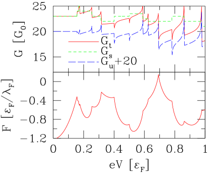
Figure 1: (Color line)The differential conductance and cohesive force of a metal cylindrical nanowire versus voltage for a nanowire with radius $k_{F}R_{0}=10.64$. Here $G_{s}$ and $G_{u}$ are the contributions from single-particle motion and interaction effect, respectively, and $G=G_{t}$ is the total differential conductance given by Eq. (8).

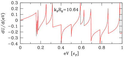
Figure 2: (Color line) The derivative of the Hartree energy $U$ with respect to the voltage.

III Cohesion and Differential Conductance

The cohesive force $F=-\left.\frac{\partial\Omega[R_{0},V,U]}{\partial L}\right|_{N_{+}}$, where the derivative is taken at constant background positive charge $N_{+}$, is given by

$$F(R_{0},V,U)=\frac{4\varepsilon_{F}}{3\lambda_{F}}\sum_{\begin{subarray}{c}\alpha=\pm\\ \nu\end{subarray}}\left(\frac{\varepsilon_{\alpha}-\varepsilon_{\nu}}{\varepsilon_{F}}\right)^{1/2}\\ \times\left[\frac{\varepsilon_{\alpha}-\varepsilon_{\nu}}{\varepsilon_{F}}+3k_{F}L\frac{\gamma_{\nu}^{2}}{k_{F}^{3}R_{0}^{3}}\left.\frac{dR_{0}}{dL}\right|_{N_{+}}\right].$$ (7)

The first term comes from the single-particle levels and the second term is due to the finite size effect. The contribution from the derivative of Hartree potential with respect to $L$ in the electronic free energy is completely canceled by that from the positive charge background, and the interactions affect the cohesive force only by shifting the chemical potentials, or equivalently by shifting the single-particle levels by an amount of the Hartree potential $U$. Therefore, the cohesion of metal nanowires is determined by the single-particle motion of the electrons, even at finite voltages.

The differential conductance $G=\frac{\partial I}{\partial V}$ is given by

$$G(R_{0},V,U)=\frac{G_{0}}{2}\sum_{\begin{subarray}{c}\alpha=\pm\\ \nu\end{subarray}}\theta\left(\varepsilon_{\alpha}-\varepsilon_{\nu}\right)\bigg{[}1-\alpha\frac{\partial U}{\partial(eV)}\bigg{]},$$ (8)

where $G_{0}=2e^{2}/h$ is the unit quantum conductance. We see that both single-particle motion and interactions contribute to the differential conductance.

The differential conductance $G$ and cohesive force as a function of voltage $V$ are shown in Fig. 1. In the figure, we have split the total differential conductance $G$ into the single-particle contribution part $G_{s}$ and the interaction contribution part $G_{u}$. At small voltages, $G=G_{s}$ and is equal to that obtained from free electron model, which is consistent with the result of linear transport. At large voltages, there are peak structures at the conductance jumps, which come from $G_{u}$. This is because at the subband thresholds, a small voltage change can induce large fluctuation of the Hartree potential, as can be seen in Fig. 2. From Fig. 1, one can also see the correlation between the variations of the conductance jumps and the force oscillation as a function of the voltage, which should be observable experimentally.

We should mention that an adequate treatment the electron-electron interactions (Hartree approximation in this work), is essential to satisfying the gauge invariance. The calculated cohesive force and differential conductance are just functions of the voltage between the two ends of the wire. This is in contrast to the results in Refs. Zagoskin, 1998 and Bogacheck et al., 2000, which depends on the partition $\beta$ of the voltage drops between the two contacts by using a charge neutrality: $N_{-}(\varepsilon_{F}+\beta eV)+N_{-}(\varepsilon_{F}-(1-\beta)eV)=2N_{-}(\varepsilon_{F})$. This treatment is clearly not self-consistent and does not satisfy the condition of gauge invariance. We should also mention that we should treat the system in the grand canonical ensemble so that the Hartree potential on the force oscillation is not double-counted, as did in Ref. van Ruitenbeck et al., 1997.

IV Magnetic Properties

We have already seen that it is very important to treat the electron-electron interactions appropriately to calculate the cohesive force and the differential conductance. The interactions can also produce significant effects in magnetic properties. By using the free electron model, the calculated magnetoconductance coefficient $\sigma$ and magnetotension coefficient $\Upsilon$ in are identically zero Zagoskin (1998). However, since the Hartree potential $U$ has to be determined self-consistently by Eq. (3) in presence of the magnetic field. As we will show that, the response of Hartree potential is sensitive to the external magnetic field at thresholds of the single-particle subbands, and gives rise non-zero magnetoconductance coefficient and magnetotension coefficient at these sub-bands. We should also show that this response of Hartree potential to the magnetic field also affects the magnetic susceptibility.

Using perturbation theory, the effect of a weak longitudinal magnetic field $H$ (i.e. a field such that the cyclotron radius $r_{c}\gg R_{0}$ perpendicular to the cross section of the wire) can be included as a spin-dependent shift of the transverse eigenvaluesZagoskin (1998)

$$\varepsilon_{\nu s}(H)=\varepsilon_{F}\left[\frac{\gamma^{2}_{\nu}}{k_{F}^{2}R_{0}^{2}}+(m_{\nu}+gm_{s})\frac{H}{H_{0}}\right],$$ (9)

where $H_{0}=k_{F}^{2}hc/2e$, $g$ is the gyro magnetic ratio factor, $c$ is the speed of light, $m_{\nu}$ is the orbital angular momentum, and $m_{s}=\pm\frac{1}{2}$ is the spin of an electron.

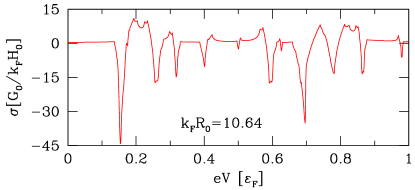
Figure 3: (Color line) The magnetoconductance coefficient $\sigma$ versus the bias voltage.

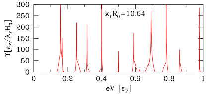
Figure 4: (Color line) The magnetotension coefficient $\Upsilon$ versus the bias voltage.

The generalized grand-canonical potential $\Omega$ and the current at weak magnetic field are modified to be

$$\Omega_{0}[R_{0},V,H]=-\frac{2\varepsilon_{F}L}{3\lambda_{F}}\sum_{\begin{subarray}{c}\alpha=\pm\\ \nu,s\end{subarray}}\left(\frac{\varepsilon_{\alpha}-\varepsilon_{\nu s}}{\varepsilon_{F}}\right)^{3/2}\!\!\!-N_{+}U,$$ (10)

and

$$I(R_{0},V,H)=\frac{2e}{h}\sum_{\nu,s}\int_{\mu_{-}-U}^{\mu_{+}-U}dE\ \theta(E-\varepsilon_{\nu s}).$$ (11)

The Hartree potential $U$ should be self-consistently determined by Eq. (3) under both voltage and the magnetic field. The cohesive force $F$ and differential conductance $G$ are also modified to be

$$F(R_{0},V,H)=\frac{2\varepsilon_{F}}{3\lambda_{F}}\sum_{\begin{subarray}{c}\alpha=\pm\\ \nu,s\end{subarray}}\left(\frac{\varepsilon_{\alpha}-\varepsilon_{\nu s}}{\varepsilon_{F}}\right)^{1/2}\\ \times\left[\frac{\varepsilon_{\alpha}-\varepsilon_{\nu s}}{\varepsilon_{F}}+3k_{F}L\frac{\gamma^{2}_{\nu}}{k_{F}^{3}R_{0}^{3}}\left.\frac{dR_{0}}{dL}\right|_{N_{+}}\right],$$ (12)

and

$$G(R_{0},V,H)=\frac{G_{0}}{4}\sum_{\begin{subarray}{c}\alpha=\pm\\ \nu,s\end{subarray}}\theta\left(\varepsilon_{\alpha}-\varepsilon_{\nu s}\right)\left[1-\alpha\frac{\partial U}{\partial(eV)}\right].$$ (13)

The calculated cohesive force and differential conductance at small magnetic field from Eqs. (12) and (13) are not much different from Eqs. (7) and (8). These two equations serve the purpose to calculate the magnetotension and magnetoconductance coefficients below.

The magnetotension coefficient $\Upsilon$ is defined as $\Upsilon=(\partial F/\partial H)_{H=0}$ and magnetoconductance coefficient $\sigma$ is defined as $\sigma=\frac{1}{L}(\partial G/\partial H)_{H=0}$. Using Eqs. (12) and (13), one gets

$$\sigma(V) =-\frac{G_{0}}{2}\sum_{\alpha=\pm}\left(1-\alpha\frac{\partial U}{\partial(eV)}\right)\left.\frac{\partial U}{\partial H}\right|_{H=0}g(\varepsilon_{\alpha})$$

$$\ \ \ \ -\frac{G_{0}}{2}\sum_{\begin{subarray}{c}\alpha=\pm\\ \nu\end{subarray}}\alpha\theta(\varepsilon_{\alpha}-\varepsilon_{\nu})\left.\frac{\partial^{2}U}{\partial H\partial(eV)}\right|_{H=0},$$ (14)

and

$$\Upsilon(V)=-\frac{2}{\lambda_{F}}\sum_{\begin{subarray}{c}\alpha=\pm\\ \nu\end{subarray}}\left[\left(\frac{\varepsilon_{\alpha}-\varepsilon_{\nu}}{\varepsilon_{F}}\right)^{-1/2}\frac{L\gamma^{2}_{\nu}}{k^{2}_{F}R^{3}_{0}}\left.\frac{\partial R_{0}}{\partial L}\right|_{N_{+}}\right.\\ +\left.\left(\frac{\varepsilon_{\alpha}-\varepsilon_{\nu}}{\varepsilon_{F}}\right)^{1/2}\right]\times\left.\frac{\partial U}{\partial H}\right|_{H=0},$$ (15)

where $g(\varepsilon_{\alpha})$ is the density of states at energy $\varepsilon_{\alpha}$ of electrons injected from reservoir $\alpha$. From these two equation, one can see that nonzero magnetotension and magnetoconductance coefficients are attributed to the response of the Hartree potential $U$ to the magnetic field.

The calculated results for $\sigma$ and $\Upsilon$ are shown in Figs. 3 and 4. Whenever there is a subband opening, there is a peak in these two coefficients. This is because the magnetic field increases the fluctuation of the Hartree potential at those subbands, which can be seen in Fig. 5.

One can consider the single-particle and interaction effects on the magnetic susceptibility which is define as $\chi=-\frac{1}{L}\left(\frac{\partial^{2}\Omega_{0}}{\partial H^{2}}\right)_{H=0}$. Using the generalized grand canonical potential Eq. (10), and keeping only the dominant part, one gets

$$\chi(eV)\approx\frac{1}{2\varepsilon_{F}\lambda_{F}}\sum_{\begin{subarray}{c}\alpha=\pm\\ \nu s\end{subarray}}\left(\frac{\varepsilon_{\alpha}-\varepsilon_{\nu s}}{\varepsilon_{F}}\right)^{-1/2}\\ \times\left.\left(\frac{\partial(U+\varepsilon_{\nu s})}{\partial H}\right)^{2}\right|_{H=0}.$$ (16)

The result is presented in Fig. 6. For nanowires with small radii $R_{0}$, $\frac{\partial U}{\partial H}$ is of the same order as $\frac{\partial\varepsilon_{\nu s}}{\partial H}=\varepsilon_{F}(m_{\nu}+gm_{s})/H_{0}$, both single-particle effect and interaction effects are important to the magnetic susceptibility. For nanowires with large $R_{0}$, $\frac{\partial U}{\partial H}$ is negligible comparing to $\frac{\partial\varepsilon_{\nu s}}{\partial H}$.

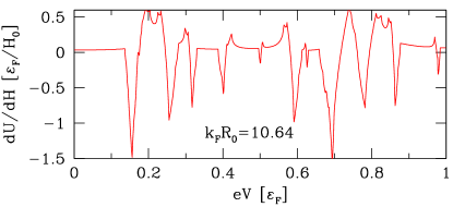
Figure 5: (Color line) The derivative of the Hartree energy $U$ with respect to the magnetic field $H$ versus the bias voltage.

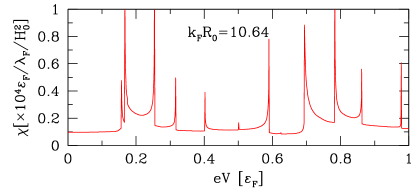
Figure 6: (Color line) The magnetic susceptibility $\chi$ versus voltage.

V Discussions and Conclusion

We should point out that based on our recent stability analysis Zhang et al. (2005), the nonzero $\sigma$ and $\Upsilon$ and the spikes of $G$ and $\chi$ usually appear in the mechanical unstable zones. However, this mechanical instability should be a problem only in the measurement of $\Upsilon$ since such a measurement is a mechanical process. The sensitivity of the Hartree potential to the applied voltage and magnetic field can be observed by measuring the differential conductance $G$, magnetoconductance coefficients and magnetic susceptibility as a function of the applied voltage as long as the measuring time is shorter than the lifetime caused by the mechanical instability.

In conclusion, we have used the generalized mean field electron model at finite voltage bias Zhang et al. (2005) to analyze the single-particle and interaction effects on the cohesion, transport and magnetic properties of cylindrical metal nanowires. At finite voltage bias, it is crucial to treat the electron-electron interactions adequately so that the calculated physical quantities are gauge invariant. Our results show that the cohesive force is determined by the single-particle effect, while the nonzero magnetotension and magnetoconductance coefficients are attribute of the response of the Hartree potential to the magnetic field. Both single-particle and interaction effects are important to the differential conductance and the magnetic susceptibility.