Fluctuation induced first-order phase transitions in a dipolar Ising ferromagnet slab

Abstract

We investigate the competition between the dipolar and the exchange interaction in a ferromagnetic slab with finite thickness and finite width. From an analytical approximate expression for the Ginzburg-Landau effective Hamiltonian, it is shown that, within a self-consistent Hartree approach, a stable modulated configuration arises. We study the transition between the disordered phase and two kinds of modulated configurations, namely, striped and bubble phases. Such transitions are of the first-order kind and the striped phase is shown to have lower energy and a higher spinodal limit than the bubble one. It is also observed that striped configurations corresponding to different modulation directions have different energies. The most stable are the ones in which the modulation vanishes along the unlimited direction, which is a prime effect of the slab’s geometry together with the competition between the two distinct types of interaction. An application of this model to the domain structure of MnAs thin films grown over GaAs substrates is discussed and general qualitative properties are outlined and predicted, like the number of domains and the mean value of the modulation as functions of temperature.

I Introduction

Magnetic phase transitions in materials with finite spacial dimensions is still a subject with many aspects to be understood and to be investigated theoretically. In these systems, one finds the competition between a strong, short-range interaction (exchange) and another weak, long-range one (dipolar), from which a modulated stable configuration is expected to outcome science . Due to the variety of possible modulated patterns, like striped, bubble and intermediate shapes, many different complex domain structures are likely to be seen. This phenomenon is observed not only in magnetic materials doniach ; allen , but also in other systems characterized by the same kind of competition between an organizing local interaction and a frustrating long-range interaction science : for example, spontaneous modulation of mesoscopic phases is found in biological systems, amphifilic solutions wu , Langmuir monolayers langmuir and block copolymers fredrickson .

There are, indeed, several analytical and numerical studies in the literature investigating size effects on the critical behaviour of magnetic systems finito_pbc1 ; finito_pbc2 ; finito_pbc3 . However, the majority of them deals with periodic boundary conditions, and not free boundaries, which comes to be the case for many materials. Even the works related to this latter kind of systems finito_Dbc1 ; finito_Dbc2 ; finito_Dbc3 do not take into account the weak, long-range (dipolar) interaction, which changes drastically the underlying physics. As shown by Garel and Doniach doniach , the inclusion of the dipolar interaction in the Ginzburg-Landau effective Hamiltonian of a magnetic slab with infinite width leads to a minimum in the Fourier space characterized by a non-zero wave vector. This is responsible not only for instability towards the spacial homogeneous phase but also for the existence of a large volume, in the Fourier space, for fluctuations of the order parameter to take place and induce a first-order transition (Brazovskii transition braso ). Therefore, to achieve a more complete understanding of finite magnetic systems, it is necessary not only to consider the finiteness of the them but also the fluctuations of the order parameter.

To explain some properties of many real materials, size effects are in fact necessary. For example, concerning non-magnetic systems, Huhn and Dohm have proposed that size effects are responsible for the temperature shift of the specific heat maximum in confined $\mathrm{He^{4}}$ finito_Dbc2 . In what concerns magnetic systems, a material that has been deeply experimentally investigated in recent years and in which size effects may play a significant role is MnAs thin films grown on GaAs mnas_prl . The reason why this heterostructure is calling so much attention is due not only to its academical appeal but also to its possible application as a spintronic device tanaka . In contrast with bulk MnAs, which presents an abrupt transition from the low temperature hexagonal (ferromagnetic) $\alpha$ phase to the high temperature orthorhombic (paramagnetic) $\beta$ phase bean , the MnAs:GaAs films show a wide region of coexistence between $\alpha$ and $\beta$ phases from approximately $0\,^{\circ}\mathrm{C}$ to $50\,^{\circ}\mathrm{C}$ kaganer ; ney ; engel ; paniago ; iikawa . In this region, periodic stripes subdivided in ferromagnetic and paramagnetic terraces arise. X-ray diffraction experiments paniago and microscopy measurements engel have shown that, while the temperature varies, the width of the ferro and paramagnetic terraces change, but the stripes remain with the same periodic width. These experiments have also brought out the terraces morphology, showing the complex phases inside the ferromagnetic terraces. As their width is of the same order of magnitude as their thickness, both spacial limitations are important to understand their internal domain structure.

Here is an outline of the article: in Section 2, we construct an expression for the Ginzburg-Landau effective Hamiltonian of a dipolar Ising ferromagnetic slab with finite width and finite thickness, considering Dirichlet boundary conditions (i.e., vanishing of the order parameter at the walls). We show that a modulated phase arises as the ordered one, and is represented by a dotted semi-ellipsis in the Fourier space as a result of frustration and Dirichlet boundary conditions. In Section 3, we apply a self-consistent Hartree calculation to take into account the fluctuations of the order parameter around the region of minimum energy. Generalizing the original method developed by Brazovskii braso to the case of this finite system, we calculate the free energy profiles for two different types of modulation: striped and bubble phases. We show that the striped phases are more stable than the bubble ones and also that the energy degeneracy concerning the region of minimum energy is broken along the finite direction. In Section 4, we discuss the application of the model to the real case of MnAs:GaAs films. Although in such systems the magnetization is rather vectorial than Ising-type, general qualitative properties due to the nature of the interactions and to the slab’s geometry can be obtained. Section 5 is devoted to the final remarks and followed by an appendix where details of some calculations are explicitly derived.

II Ginzburg-Landau for the finite slab

We consider a slab with thickness $D$ ($z$ axis), width $d$ ($x$ axis) and no limitation along the $y$ axis; the magnetization is supposed to point only to the $\hat{z}$ direction (Ising model) and to depend upon $x$ and $y$ only (uniform along $\hat{z}$). This is, indeed, a very simplified model of a ferromagnetic stripe on the MnAs:GaAs coexistence region, but we will postpone this discussion until the last section. Our purpose in this section is to obtain a two-dimensional Ginzburg-Landau to describe the system; first, consider the well-known mean field expansion of the free energy due to the exchange interaction negele :

$$F_{exch}[m]=D\int d^{2}rf_{exch}\,,$$ (1)

where

$$f_{exch}=\frac{T_{c}}{16a}\left|\vec{\nabla}m\right|^{2}+\frac{(T-T_{c})}{2a^{3}}m^{2}+\frac{T_{c}}{12a^{3}}m^{4}\,.$$ (2)

$T_{c}$ is the Ising ferromagnetic critical temperature, $a$ is the lattice parameter and $m(\vec{r})$, the scalar order parameter, is the coarse-grained spin in the position $\vec{r}=(x,y)$. We are denoting, through all this article, the integrals over the region limited by the plane of the slab as:

$$\int d^{2}r=\int_{-\infty}^{\infty}\int_{0}^{d}dxdy\,.$$

For the sake of simplicity, we consider a cubic lattice. In the long wavelength limit, the actual crystallographic structure will not change significantly the basic physical properties of the system. In this limit, we can calculate the dipolar contribution to the total energy $f_{dip}$ using just Maxwell equations.

To obtain $f_{dip}$, we express the magnetization $M(\vec{r})$ at the position $\vec{r}$ in terms of its Fourier components as

$$M(\vec{r})=\frac{g\mu_{B}}{a^{3}}\sum_{n>0,q_{y}}m_{n,q_{y}}\sin\left(\frac{n\pi x}{d}\right)e^{-iq_{y}y}\,,$$ (3)

where $g$ is the gyromagnetic factor, $\mu_{B}$ is the Bohr magneton and:

$$m_{n,q_{y}}=\frac{2}{dL_{y}}\int_{0}^{d}\int_{-\infty}^{\infty}m(\vec{r})\sin\left(\frac{n\pi x}{d}\right)e^{iq_{y}y}dxdy\,.$$ (4)

In expression (3), the sine term appears as a consequence of the boundary condition that the magnetization vanishes at the edges of the slab (Dirichlet boundary conditions). In what concerns MnAs:GaAs thin films, this condition approximates the fact that, in the coexistence region, the ferromagnetic terraces are succeeded by paramagnetic ones.

As we show in Appendix A, the magnetostatic energy of the arbitrary configuration (3) can be straightforward calculated from Maxwell equations, yielding:

$$f_{dip}=\left(\frac{g\mu_{B}}{a^{3}}\right)^{2}\sum_{q_{y},n,n^{\prime}}4\pi^{2}nn^{\prime}m_{n,q_{y}}m_{n^{\prime},-q_{y}}p\int_{0}^{\infty}du\frac{\left(1-e^{-\frac{1}{p}\sqrt{u^{2}+(q_{y}d)^{2}}}\right)\left[1+(-1)^{nn^{\prime}+1}\cos(u)\right]}{\sqrt{u^{2}+(q_{y}d)^{2}}\left(u^{2}-n^{2}\pi^{2}\right)\left(u^{2}-n^{\prime 2}\pi^{2}\right)}\,,$$ (5)

where the sums are over $n$ and $n^{\prime}$ with same parity and where we have denoted the slab’s aspect ratio as $p=d/D$. As we wish a simple model to describe the main physical properties of the slab, we look for an analytical approximation for (5). Disregarding the cross terms, which are usually negligible, we have that the sum of the direct terms is:

$$f_{dip}=\left(\frac{g\mu_{B}}{a^{3}}\right)^{2}\sum_{n,q_{y}}\pi\frac{\left(1-e^{-qD}\right)}{qD}m_{n,q_{y}}m_{n,-q_{y}}\,,$$ (6)

where we denoted the wave vector modulus by:

$$q=\sqrt{\frac{n^{2}\pi^{2}}{d^{2}}+q_{y}^{2}}\,.$$ (7)

The accuracy of the approximation (6) depends on the values of the parameters involved and on the pair $(n,q_{y})$ considered. In the experimental case of interest, namely, the MnAs:GaAs films in the neighbourhood of the phase transition between the ordered and disordered phases, this approximation implies in errors less than $20\%$ as long as $p>0.5$.

The approximate analytical expression obtained is very similar to the expression deduced by Garel and Doniach for a slab with infinite width doniach . The only difference is that, in the present case, the wave vector component along the $x$ direction is discrete due to the slab’s finite width. It is clear that in the limit $d\rightarrow\infty$ we recover the same expression.

Using equation (6), we obtain the following expression for the total free energy density

$$f_{tot}=\sum_{n>0,q_{y}}\left[\frac{T-T_{c}}{4a^{3}}+f(q)\right]m_{n,q_{y}}m_{n,-q_{y}}+\frac{T_{c}}{96a^{3}}\sum_{\{n_{i}\},\{q_{i}\}}m_{\{n_{1},n_{2},n_{3}\},-q_{1}-q_{2}-q_{3}}m_{n_{1},q_{1}}m_{n_{2},q_{2}}m_{n_{3},q_{3}}\,,$$ (8)

where

$$f(q)=\frac{T_{c}q^{2}}{32a}+\left(\frac{g\mu_{B}}{a^{3}}\right)^{2}\pi\frac{\left(1-e^{-qD}\right)}{qD}\,,$$ (9)

and

$$\left\langle m\right\rangle_{\{n_{1},n_{2},n_{3}\},-q_{1}-q_{2}-q_{3}} = \left(\left\langle m\right\rangle_{n_{1}+n_{2}-n_{3}}+\left\langle m\right\rangle_{n_{1}-n_{2}+n_{3}}+\left\langle m\right\rangle_{-n_{1}+n_{2}+n_{3}}-\left\langle m\right\rangle_{n_{1}+n_{2}+n_{3}}\right.$$ (10)

$$\left.-\left\langle m\right\rangle_{n_{1}-n_{2}-n_{3}}-\left\langle m\right\rangle_{-n_{1}+n_{2}-n_{3}}-\left\langle m\right\rangle_{-n_{1}-n_{2}+n_{3}}\right)_{,-q_{1}-q_{2}-q_{3}}\,.$$

The quartic term is the same as those obtained in previous works about finite systems with Dirichlet boundary conditions (see, for instance, finito_Dbc1 ; finito_Dbc3 ). The effects of the two interactions mentioned before are evident from (9): while the $q^{2}$ term, generated by the exchange energy, favours $q=0$ (non-modulated) configurations, the last term, generated by the dipolar energy, favours $q\rightarrow\infty$ configurations. The total energy reaches its minimum value when the wave vector modulus is given by (as long as $q_{0}D\gg 1$):

$$q_{0}=\frac{1}{a}\left(\frac{16\pi g^{2}\mu_{B}^{2}}{T_{c}Da^{2}}\right)^{1/3}\,,$$ (11)

which means that the most relevant thermodynamic states are characterized by a non-zero modulation ($q_{0}\neq 0$). Expression (11) is the same as the one obtained by Garel and Doniach in doniach for the minimum energy of the infinite slab; however, in their case, the phase space of low energy excitations is described a circle in the Fourier space, whereas in the present situation it is described by a dotted semi-ellipsis in the $(n,q_{y})$ space, as it is shown in figure 1.

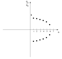
(a)                                       (b)

Figure 1: Region on the momentum (Fourier) space corresponding to the minimum of the Ginzburg-Landau for the case of a slab with (a) infinite width and (b) finite width.

Expanding (8) around its minimum, it is straightforward to obtain the respective partition function:

$$Z=\int\mathcal{D}m\exp\left(-\mathcal{H}[m]\right)\,,$$ (12)

where the Ginzburg-Landau effective Hamiltonian $\mathcal{H}$ is given by:

$$\mathcal{H}[m] = \frac{1}{2}\int\int d^{2}rd^{2}r^{\prime}m(\vec{r})G_{0}^{-1}(\vec{r},\vec{r}^{\prime})m(\vec{r}^{\prime})$$ (13)

$$+\frac{u}{4}\int d^{2}rm^{4}(\vec{r})\,,$$

and the correlation function $G_{0}$ is written in terms of its Fourier series as:

$$G_{0}^{-1}(\vec{r},\vec{r}^{\prime}) = \frac{1}{\pi d}\sum_{n>0}\int dq_{y}\left.G_{n,q_{y}}^{(0)}\right.^{-1}\sin\left(\frac{n\pi x}{d}\right)\sin\left(\frac{n\pi x^{\prime}}{d}\right)e^{-iq_{y}(y-y^{\prime})}\,,$$

$$\left.G_{n,q_{y}}^{(0)}\right.^{-1} = \frac{1}{r_{0}+c\left(q-q_{0}\right)^{2}}\,.$$ (14)

The parameters $u$, $r_{0}$ and $c$ appearing in the above expressions can be written in terms of the microscopic parameters of the systems as:

$$u = \frac{DT_{c}}{3a^{3}T}\,,$$

$$r_{0} = \frac{\left(T-T^{*}\right)D}{a^{3}T}\,,$$

$$c = \frac{3DT_{c}}{8aT}\,,$$ (15)

where we defined the shifted critical temperature:

$$T^{*}=T_{c}\left[1-6\left(\frac{\pi g^{4}\mu_{B}^{4}}{16D^{2}a^{4}T_{c}^{2}}\right)^{1/3}\right]\,.$$ (16)

Therefore, considering the expression for the correlation function, (14), it is expected some similarity between this system and the Brazovskii’s model braso . The question is if the reduction in the momentum (Fourier) space, due to the discreteness of the $x$ components ($q_{x}=n\pi/d$), is able to substantially change the picture, since Garel and Doniach have shown that, for the case of an infinite slab, in which $q_{x}$ is continuous, a fluctuation induced first-order phase transition does occur between the ordered (modulated) and the disordered phase doniach .

III Hartree calculation and Brazovskii’s procedure

As we detailed in the previous section, there is a degenerate region at the Fourier space, expressed by the non-zero wave vector modulus $q_{0}$, corresponding to the minimum of the Ginzburg-Landau effective Hamiltonian. Hence, there is a large space for fluctuations of the order parameter to take place, and a mean-field approach to calculate the partition function (12) - and its corresponding thermodynamical properties - is not satisfactory. To deal with that, we generalize the procedure adopted by Brazovskii braso to our finite system. Such procedure is based on the Hartree self-consistent method, that consists on replacing the quartic term by an effective quadratic one lubenski :

$$\frac{u}{4}\int d^{2}rm^{4}(\vec{r})\rightarrow\frac{3u}{2}\int d^{2}r\left\langle m^{2}(\vec{r})\right\rangle m^{2}(\vec{r})\,.$$ (17)

Then, using the identity

$$\left\langle m^{2}(\vec{r})\right\rangle=G(\vec{r},\vec{r})+\left\langle m(\vec{r})\right\rangle^{2}\,,$$

and substituting in (13), it is clear that a self-consistent equation is obtained for the correlation function:

$$G^{-1}(\vec{r},\vec{r}^{\prime}) = G_{0}^{-1}(\vec{r},\vec{r}^{\prime})+3uG(\vec{r},\vec{r})\delta(\vec{r}-\vec{r}^{\prime})+$$ (18)

$$+3u\left\langle m(\vec{r})\right\rangle^{2}\delta(\vec{r}-\vec{r}^{\prime})\,,$$

where the Dirac delta function is to be understood as belonging to the intervals $[0,d]$ ($x$ axis) and $[-\infty,\infty]$ ($y$ axis), and not to $[-\infty,\infty]$ and $[-\infty,\infty]$, as it is usually assumed.

Following Brazovskii, the dominant contributions for the correlation function $G(\vec{r},\vec{r}^{\prime})$ come from the diagonal Fourier components $G_{(n,q_{y}),(n,-q_{y})}$ such that $\sqrt{n^{2}\pi^{2}/d^{2}+q_{y}^{2}}=q_{0}$. Therefore, it is useful to write the self-consistent equation on the Fourier space

$$G_{n,q_{y}}^{-1} = \left.G_{n,q_{y}}^{(0)}\right.^{-1}+\frac{3u}{2}\left\langle G\right\rangle+\frac{3u}{4}\left\langle G\right\rangle_{n}+\frac{9u}{4}\sum_{p_{y}}\left\langle m\right\rangle_{n,p_{y}}\left\langle m\right\rangle_{n,-p_{y}}-\frac{3u}{4}\sum_{p_{y}}\left\langle m\right\rangle_{n,p_{y}}\left\langle m\right\rangle_{3n,-p_{y}}+$$ (19)

$$\frac{3u}{4}\sum_{m\neq n,p_{y}}\left\langle m\right\rangle_{m,p_{y}}\left[2\left\langle m\right\rangle_{m,-p_{y}}-\left\langle m\right\rangle_{m+2n,-p_{y}}+\left\langle m\right\rangle_{2n-m,-p_{y}}-\left\langle m\right\rangle_{m-2n,-p_{y}}\right]\,,$$

where

$$\left\langle G\right\rangle_{m} = \frac{1}{\pi d}\int dp_{y}G_{m,p_{y}}\,,$$

$$\left\langle G\right\rangle = \sum_{m}\left\langle G\right\rangle_{m}\,.$$ (20)

The summation in (19) is over the region comprehended by the dotted semi-ellipsis shell whose thickness $\Lambda$ is such that $\Lambda\ll q_{0}$. In this region, the diagonal Fourier components $G_{n,q_{y}}$ can be expanded as:

$$G_{n,q_{y}}=\frac{1}{r+c\left(q-q_{0}\right)^{2}}$$ (21)

and their mean values can be evaluated to yield

$$\left\langle G\right\rangle_{n} = \frac{4q_{0}}{\pi\sqrt{c}\sqrt{r}}\frac{1}{\sqrt{\frac{q_{0}^{2}d^{2}}{\pi^{2}}-n^{2}}}\,,$$

$$\left\langle G\right\rangle = \frac{4q_{0}}{\pi\sqrt{c}\sqrt{r}}\sum_{m=1}^{N\left(q_{0}d/\pi\right)}\frac{1}{\sqrt{\frac{q_{0}^{2}d^{2}}{\pi^{2}}-m^{2}}}\,.$$ (22)

Here $N(x)$ denotes the integer closest to $x$ and smaller than $x$. Therefore, equation (19) can be written as:

$$r = r_{0}+\frac{\Gamma_{n}u}{\sqrt{r}}+\frac{9u}{4}\sum_{p_{y}}\left\langle m\right\rangle_{n,p_{y}}\left\langle m\right\rangle_{n,-p_{y}}-\frac{3u}{4}\sum_{p_{y}}\left\langle m\right\rangle_{n,p_{y}}\left\langle m\right\rangle_{3n,-p_{y}}+$$ (23)

$$\frac{3u}{4}\sum_{m\neq n,p_{y}}\left\langle m\right\rangle_{m,p_{y}}\left[2\left\langle m\right\rangle_{m,-p_{y}}-\left\langle m\right\rangle_{m+2n,-p_{y}}+\left\langle m\right\rangle_{2n-m,-p_{y}}-\left\langle m\right\rangle_{m-2n,-p_{y}}\right]\,,$$

where:

$$\Gamma_{n}=\frac{6q_{0}}{\pi\sqrt{c}}\sum_{m=1}^{N\left(q_{0}d/\pi\right)}\frac{\left(1+\frac{\delta_{m,n}}{2}\right)}{\sqrt{\frac{q_{0}^{2}d^{2}}{\pi^{2}}-m^{2}}}\,.$$ (24)

It is clear that the self-consistent equation for the renormalized parameter $r$ , equation (23), depends on the system phase through $\left\langle m(\vec{r})\right\rangle$. However, for any configuration $\left\langle m(\vec{r})\right\rangle$, analogously to braso , the equation does not allow the solution $r=0$, what implies that the transition from the disordered to this ordered phase (characterized by the mean value $\left\langle m(\vec{r})\right\rangle$) is not second-order. Therefore, a first-order transition is expected, as well as the raise of metastable states (and the respective spinodal stability limits).

To further investigate how the system achieves all the possible distinct modulated states, it is useful to calculate the free energy difference between these configurations and the disordered one. Hence, we use the same procedure as Brazovskii and consider that the conjugate field $h$ grows from zero in the disordered phase to a maximum value and then goes again to zero in the ordered stable phase, characterized by an amplitude $A\neq 0$ braso :

$$\Delta F=F_{ord}-F_{desord}=\int_{0}^{A}\frac{dF}{dA^{\prime}}dA^{\prime}=\int_{r}^{r_{A}}\left(\sum_{n,q}\frac{\delta F}{\delta\left\langle m\right\rangle_{n,q}}\frac{d\left\langle m\right\rangle_{n,q}}{dA}\right)\frac{dA}{dr^{\prime}}dr^{\prime}\,,$$ (25)

where

$$\frac{\delta F}{\delta\left\langle m\right\rangle_{n,q}}=h_{n,q}$$

is the conjugate field in the Fourier space. A lengthy but straightforward calculation gives:

$$h_{n,q} = G_{n,q}^{-1}\left\langle m\right\rangle_{n,q}+\frac{u}{4}\sum_{m,m^{\prime},p,p^{\prime}}\left\langle m\right\rangle_{m,p}\left\langle m\right\rangle_{m^{\prime},p^{\prime}}\left\langle m\right\rangle_{\{m,m^{\prime},n\},q-p-p^{\prime}}-$$ (26)

$$\frac{9u}{4}\left\langle m\right\rangle_{n,q}\sum_{p}\left\langle m\right\rangle_{n,p}\left(\left\langle m\right\rangle_{n,-p}-\frac{1}{3}\left\langle m\right\rangle_{3n,-p}\right)-$$

$$\frac{3u}{4}\left\langle m\right\rangle_{n,q}\sum_{m\neq n,p}\left\langle m\right\rangle_{m,p}\left[2\left\langle m\right\rangle_{m,-p}-\left\langle m\right\rangle_{m+2n,-p}+\left\langle m\right\rangle_{2n-m,-p}-\left\langle m\right\rangle_{m-2n,-p}\right]-$$

$$\frac{3u}{4}\left\langle G\right\rangle_{3n}\left\langle m\right\rangle_{3n,q}+\frac{3u}{4}\sum_{m\neq n}\left\langle G\right\rangle_{m}\left(-\left\langle m\right\rangle_{n+2m,q}+\left\langle m\right\rangle_{2m-n,q}-\left\langle m\right\rangle_{n-2m,q}\right)\,.$$

We follow Garel and Doniach doniach and study two different modulated configurations: the striped and the bubble phases.

Striped phases

The name stripes may be somehow misleading, as genuine stripes cannot be formed due to the boundary conditions, unless they lie only along the $y$ direction. In fact, these phases refer to the simplest modulated configuration that can arise in the finite system:

$$\left\langle m\right\rangle_{n,q} = A\delta_{n,n_{0}}\left(\delta_{q,q_{0y}}+\delta_{q,-q_{0y}}\right)$$ (27)

$$\left\langle m\left(\vec{r}\right)\right\rangle = 2A\sin\left(\frac{n_{0}\pi x}{d}\right)\cos\left(q_{0y}y\right)\,,$$ (28)

where

$$\sqrt{\frac{n_{0}^{2}\pi^{2}}{d^{2}}+q_{0y}^{2}}=q_{0}\,.$$

Therefore, the use of the name stripes is to make contact with the phases of the infinite slab rather than to describe exactly the geometrical pattern. Figure 2 compares the general picture of the simplest modulated phases of the infinite and of the finite slab.

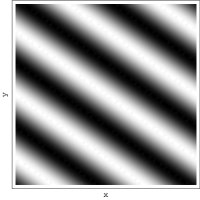
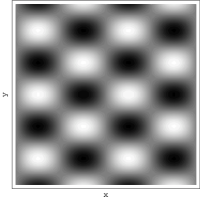
(a)                                       (b)

Figure 2: Contour plot of the order parameter along the slab’s plane concerning the simplest modulated phases that arise in the case of (a) an infinite slab and (b) a finite slab.

Substituting equation (28) in expressions (23) and (26), we obtain the following expressions for the self-consistent and the state equations:

$$r = r_{0}+\frac{\Gamma_{n_{0}}u}{\sqrt{r}}+\frac{9}{2}uA^{2}\,,$$

$$h = rA-\frac{9}{4}uA^{3}\,.$$ (29)

Imposing that the conjugate field vanishes in the ordered phase (denoted by $r_{A}$), we get:

$$-r_{A}=r_{0}+\frac{\Gamma_{n_{0}}u}{\sqrt{r}}\,.$$ (30)

This equation is the same as the one obtained for the case of an infinite slab, and was considered by Brazovskii in his original work. It implies that these striped phases can arise as metastable states below the spinodal stability limit:

$$r_{spinodal}\approx-1.89\left(u\Gamma_{n_{0}}\right)^{2/3}\,.$$

To obtain the free energy difference between these modulations and the disordered phase, we take $\left\langle m\left(\vec{r}\right)\right\rangle=0$ in (23); we get:

$$r=r_{0}+\frac{\Gamma_{n_{0}}u}{\sqrt{r}}\,.$$ (31)

Using (25), the free energy difference is

$$\Delta F_{s}=\frac{2\left(u\Gamma_{n_{0}}^{4}\right)^{1/3}}{9}\left[-\frac{\rho_{A}^{2}}{2}-\frac{\rho^{2}}{2}-\sqrt{\rho}+\sqrt{\rho_{A}}\right]\,,$$ (32)

where we defined the auxiliary variables

$$\rho_{i}=\frac{r_{i}}{\left(u\Gamma_{n_{0}}\right)^{2/3}}\,.$$ (33)

The new feature that appears as a consequence of the finiteness of the system is the dependence of the factor $\Gamma_{n_{0}}$ with respect to the slab’s width $d$ and to the modulation label $n_{0}$, which indicates what point of the semi-ellipsis is taken to modulate the system. It is clear that a modulation labeled by $n_{0}$ can arise only if:

$$\frac{q_{0}d}{\pi}\geq n_{0}$$ (34)

otherwise the semi-ellipsis does not comprehend this specific point. Such label can be interpreted as the number of “spread” domains along the $x$ direction, since there are no sharp walls and the magnetization changes sign continuously from one domain to another.

From the definition of $\Gamma_{n_{0}}$, equation (24), it is clear that when the ratio $q_{0}d/\pi$ is an integer the factor diverges. However, this does not mean that the free energy difference diverges, since the spinodal limit also depends upon $\Gamma_{n_{0}}$. A plot of this energy as a function of the ratio $q_{0}d/\pi$ for a given temperature is shown in figure 3. Firstly, it is clear that there are barriers in the energy profile whenever:

$$\frac{q_{0}d}{\pi}\in\mathbb{Z}$$ (35)

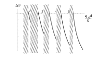
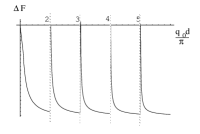
(a)                                       (b)

Figure 3: General behaviour of the free energy difference between the striped phase ($n_{0}=1$) and the disordered phase as a function of the ratio $q_{0}d/\pi$. The temperature in (a) is greater than the temperature in (b). The shaded regions indicate that the ordered state is not metastable (temperature above the spinodal) and therefore it does not make sense to define a free energy difference.

We also note that, as the temperature decreases, the barriers heights become approximately uniform. Another important consequence of the $\Gamma_{n_{0}}$ dependence upon $n_{0}$ is the break of the semi-ellipsis degeneracy. In a mean-field approach, all the different modulations that can exist for a certain slab’s width $d$ would have the same energy. However, as shown in figure 4, when we take into account the fluctuations, each modulation $n_{0}$ assumes distinct energy values, implying that the high degeneracy of the minimum energy is broken. Moreover, as the slab’s width increases ($d\rightarrow\infty$), the energies get closer again, what agrees with the result for the infinite slab, where there is no degeneracy break.

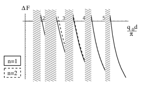
Figure 4: General behaviour of the free energy difference between the ordered and the disordered states concerning the striped phase with $n_{0}=1$ (full line) and the striped phase with $n_{0}=2$ (dashed line). The shaded regions indicate that the ordered state is not metastable (temperature above the spinodal) and therefore it does not make sense to define a free energy difference.

A deeper analysis reveals that, in fact, only the degeneracy along the $q_{x}$ direction is broken, and not the other along the $q_{y}$ direction. This is only a reflection of the translational invariance break along the $x$ direction, due to the existence of edges.

It is important to analyze carefully the energy barriers that appear when condition (35) is met, because in such situation (and only in it) genuine stripes, characterized by modulation only along the $x$ direction, can appear. This configuration is given by

$$\left\langle m\right\rangle_{n,q} = A\delta_{n,n_{0}}\delta_{q,0}$$ (36)

$$\left\langle m\left(\vec{r}\right)\right\rangle = A\sin\left(\frac{n_{0}\pi x}{d}\right)$$ (37)

and does not obey to the same Hartree or state equations of the configurations previously considered. Indeed, a direct substitution of (37) in (23) and (26) imply that:

$$r = r_{0}+\frac{\Gamma_{n_{0}}u}{\sqrt{r}}+\frac{9}{4}uA^{2}\,,$$

$$h = rA-\frac{3}{2}uA^{3}\,.$$ (38)

Hence, the self-consistent equation is given by:

$$-\frac{r_{A^{\prime}}}{2}=r_{0}+\frac{\Gamma_{n_{0}}u}{\sqrt{r_{A^{\prime}}}}$$ (39)

and the free energy difference by:

$$\Delta F_{s^{\prime}}=\frac{2\left(u\Gamma_{n_{0}}^{4}\right)^{1/3}}{9}\left[-\frac{\rho_{A^{\prime}}^{2}}{4}-\frac{\rho^{2}}{2}-\sqrt{\rho}+\sqrt{\rho_{A^{\prime}}}\right]\,.$$ (40)

A plot comparing the energy profiles of the “general” stripes and the stripes with no modulation along the $y$ direction is shown in figure 5. It is clear that the latter is always more stable than the former; however, it is important to bear in mind that the genuine stripes can only appear when condition (35) is fulfilled. The spinodal limit for them is given approximately by $-1.5\left(u\Gamma_{n_{0}}\right)^{2/3}$, what means that these configurations always appear before the “general stripes”. Therefore, we can say that whenever the geometric condition (35) is met and the system can be divided in non-modulated configurations along the $y$ direction, it will do.

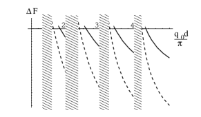
Figure 5: General behaviour of the free energy difference between the ordered and disordered states concerning the “general” striped phase ($n_{0}=1$ - full line) and the genuine striped phase with no modulation along the $y$ direction ($n_{0}=1$ - dashed line) as a function of the ratio $q_{0}d/\pi$. The shaded regions indicate that the ordered state is not metastable (temperature above the spinodal) and therefore it does not make sense to define a free energy difference.

Bubble phases

In an infinite slab, where the wave vector components $q_{x}$ and $q_{y}$ are continuous, an hexagonal bubble phase is described by the configuration doniach :

$$\sum_{i=1}^{3}\cos\left(\vec{k}_{i}\cdot\vec{r}\right),\quad\sum_{i=1}^{3}\vec{k}_{i}=0\;\mathrm{and}\;\left|\vec{k}_{i}\right|=q_{0}\,.$$ (41)

It is clear that such condition can no longer be satisfied by the finite slab, due to the boundary conditions. Than, to study other phases than the simplest “striped” ones, we consider a phase that resembles some aspects of the bubbles in the infinite slab, as shown in figure 6:

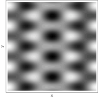
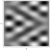
(a)                                       (b)

Figure 6: Contour plot of the order parameter along the slab’s plane concerning the “bubble” phases that arise in the case of (a) an infinite slab and (b) a finite slab.

$$\left\langle m\right\rangle_{n,q} = A\left(\delta_{n,n_{0}}\delta_{q,q_{0y}}+\delta_{n,n_{0}}\delta_{q,-q_{0y}}+\delta_{n,n_{0}+1}\delta_{q,q_{1y}}+\delta_{n,n_{0}+1}\delta_{q,-q_{1y}}\right)\,,$$

$$\left\langle m\left(\vec{r}\right)\right\rangle = A\sin\left(\frac{n_{0}\pi x}{d}\right)\cos\left(q_{0y}y\right)+A\sin\left(\frac{\left(n_{0}+1\right)\pi x}{d}\right)\cos\left(q_{1y}y\right)\,,$$ (42)

where:

$$\sqrt{\frac{n_{0}^{2}\pi^{2}}{d^{2}}+q_{0y}^{2}}=\sqrt{\frac{(n_{0}+1)^{2}\pi^{2}}{d^{2}}+q_{1y}^{2}}=q_{0}\,.$$ (43)

Once more, we adopt the name bubbles to keep the correspondence to the case of the infinite slab, and not to describe the actual geometric pattern. We note that this configuration can take place as long as:

$$\frac{q_{0}d}{\pi}\geq n_{0}+1\,.$$ (44)

Substituting expression (42) in (23) and (26) yields the following Hartree and state equations:

$$r = r_{0}+\frac{\Gamma_{n_{0}}u}{\sqrt{r}}+\frac{15}{2}uA^{2}\,,$$

$$h = rA-\frac{9}{4}uA^{3}\,.$$ (45)

Since the conjugate field vanishes in the ordered bubble state, we obtain, for the self-consistent equation:

$$-\frac{7}{3}r_{A}=r_{0}+\frac{\Gamma_{n_{0}}u}{\sqrt{r_{A}}}\,.$$ (46)

The spinodal is approximately $-2.51\left(u\Gamma_{n_{0}}\right)^{2/3}$, what means that this configuration appears after the striped phases. In a mean-field calculation, they (and any other modulation characterized by $q_{0}$) would appear simultaneously for both the infinite and the finite slab. Therefore, the fluctuations break also this degeneracy, but this is not an effect due to the finiteness of the system, since it occurs also for the infinite slab.

Using (45) and (46), the energy difference is calculated as:

$$\Delta F_{b}=\frac{4\left(u\Gamma_{n_{0}}^{4}\right)^{1/3}}{15}\left[-\frac{7\rho_{A}^{2}}{6}-\frac{\rho^{2}}{2}-\sqrt{\rho}+\sqrt{\rho_{A}}\right]\,.$$ (47)

As it is the case for the striped phases, energy barriers are observed when condition (35) is met and, for different values of the label $n_{0}$, different values of energy are observed. Figure 7 compares the energy difference of this bubble phase with the one referring to the striped phase; we note that, in general, the former is greater than the latter, what means that the simplest modulation is more stable. Moreover, since the bubble’s spinodal is lower than the stripe’s spinodal, we expect that the magnetic domain configuration will never be divided into bubbles.

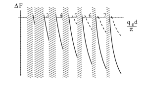
Figure 7: General behaviour of the free energy difference between the ordered and disordered states concerning the striped (full line) and the bubble phase (dashed line), both with $n_{0}=1$, as a function of the ratio $q_{0}d/\pi$. The shaded regions indicate that the ordered state is not metastable (temperature above the spinodal) and therefore it does not make sense to define a free energy difference.

This picture can change in the presence of an external magnetic field along the $z$ direction. As showed by Garel and Donicah doniach in the case of the infinite slab, in a mean-field approach, the magnetic field can favour the formation of bubbles instead of stripes for certain temperature ranges. We expect that, in the present case of the finite slab in the Hartree self-consistent approach, a similar phenomenon can occur. However, since this is not the scope of this work, we do not investigate further such subject .

More complex patterns built up from other combinations of the semi-ellipsis points are also possible; however, the calculations involved become more difficult. From the previous analysis, we expect that the simplest modulation will be the most stable one, as it is the case for the infinite slab. The main difference is that, in the latter case, the spinodal of more complex phases are greater, and not lower, than the spinodal of the simplest modulation.

IV Applications to $MnAs:GaAs$ films

The aspects presented in the last section are particularly interesting on systems in which the slab’s width $d$ can be varied. In fact, this is the case for MnAs thin films grown over GaAs substrates, where it is observed the formation of ferromagnetic terraces whose widths depends almost linearly upon the temperature paniago :

$$d(T)=600-12T\,,$$ (48)

where $d$ is given in nanometers and $T$ in Celsius degrees. This is valid in the region where the ferromagnetic terraces coexist with the paramagnetic stripes, from $0\,^{\circ}\mathrm{C}$ to $50\,^{\circ}\mathrm{C}$. In this section, we intend to discuss the domain structures inside the ferromagnetic terraces, considering them as finite slabs, and compare to experimental results.

It is important to notice that, in the MnAs:GaAs system, the spins responsible for the magnetism are not scalar (Ising-like), but vector (due to the crystalline field, they would be better described by a $xz$ model, and an approach following the lines of pokrovsky would be necessary). Besides, the film thickness is larger than $100\,\mathrm{nm}$, what means that three dimensional domains could be formed. Nonetheless, as we are concerned with the general picture of the problem, we believe that this simple model proposed can outline some general properties due to the nature of the competing interactions (strong short-range versus weak long-range) and to the geometry involved (Dirichlet boundary conditions in Cartesian coordinates). However, the specific features of the domains that would be formed can be much more complex, as we showed previously for the case of one-dimensional Néel walls fernandes .

First of all, we need to estimate the order of magnitude of the parameters. We do not intend to obtain an exact quantitative description, but rather some qualitative insights about the domain structure of each ferromagnetic terrace. Therefore, based on the experimental studies regarding MnAs:GaAs thin films kaganer ; ney ; engel ; paniago ; iikawa , we take $a=5\,\textrm{\r{A}}$, $g=3$, $D=130\,\mathrm{nm}$ and $T_{c}=32\,\mathrm{meV}$.

Substituting these values in the equations deduced in the previous sections, we can study the behaviour of striped and bubble phases inside the ferromagnetic terraces. Figure 8 shows the energy difference between the striped phases and the paramagnetic (disordered) phase. We note that the temperature is always below the spinodal limit and that there are local energy minima referring to the configurations in which there is no modulation along the $y$ direction. Such configurations comprehend structures from $1$ (the last energy minimum) to $10$ (the first energy minimum) “spread” domains lying along the $x$ direction. Note that, for a real system, in which there are impurities and the various ferromagnetic terraces do not have exactly the same width at a given temperature, these local minima would not be so sharp and the free energy profile would be continuous, as sketched in the figure.

We also see that, when $T\approx 45\,^{\circ}\mathrm{C}$ ($d\approx 550\,\mathrm{nm}$), the semi-ellipsis at the Fourier space representing the minimum energy does not comprehend any positive and integer $n$, what means that the modulated state cannot arise anymore. Above this temperature, it is likely that the interaction between neighbour ferromagnetic terraces will play an important role to determine the new stable configurations.

Figure 8: Free energy difference between the striped and the disordered phases for MnAs:GaAs films as a function of temperature (in Celsius degrees). The sharp minima refer to the configurations for which there is no modulation along the $y$ direction and $n$ domains along the $x$ direction, where $n$ goes from $10$ (first minimum) to $1$ (last minimum). Contour plots for some of these configurations are presented, as well as a sketch of this profile in the case of a real system.

Another aspect that is not represented explicitly in the figure is that the break of degeneracy between states corresponding to different number of domains $n$ is very weak, since the energy scales involved are experimentally unnoticeable. This is due not only to the large value of the slab’s thickness $D$ but also due to the fact that the temperature is far below the spinodal limit. Therefore, in the beginning, when the temperature is just above $0\,^{\circ}\mathrm{C}$, all configurations with $n\leq 10$ and non-zero $q_{y}$ (such that the wave vector modulus is $q_{0}$) are degenerate. As the temperature increases, the system meets the first local free energy minimum, corresponding to $n=10$. Hence, at this temperature, the terrace will be divided in $10$ domains along the $x$ direction and no modulation along the $y$ direction. In the sequence, all configurations with $n\leq 9$ and $q_{y}\neq 0$ are again degenerate; however, since the system was previously in a $10$ domain configuration, it will be energetically favourable to “destroy” just one domain along the $x$ direction before it meets the local minimum corresponding to $n=9$. Therefore, we expect that each local free energy minimum corresponds to a change in the number of domains along the $x$ direction, and that, for these specific temperatures (where the free energy has these local “traps”) , the configurations will be non-modulated along the $y$ direction.

An experimental measure that can show the occurrence of these local free energy minima is the mean value of $q_{y}$, the $y$-component of the modulation, that can be obtained by x-ray scattering. As we have already pointed out, in a real sample not all the ferromagnetic slabs will have the same width determined by (48). Instead, we can consider, as in coelho , a Gaussian distribution for the widths, in which the mean width is given by (48). Figure 9 shows the behaviour of $\left\langle q_{y}\right\rangle$ as a function of temperature for a Gaussian distribution whose mean standard variation is $5\%$ of the mean width. Note that the local minima referring to the configurations whose number of domains along the $x$ axis is large are almost suppressed, while the minima correspondent to a small number of domains are more pronounced.

Figure 9: Mean value of the MnAs:GaAs films modulation along the $y$ direction, in units of $10^{3}\textrm{\r{A}}^{-1}$, as a function of the temperature in Celisus degrees. A Gaussian distribution is considered for the widths of the sample’s terraces.

This prediction for the qualitative behaviour of $\left\langle q_{y}\right\rangle$ is a consequence only of the competition between the interactions involved (which generates the semi-ellipsis at the phase space) and of the geometry considered (since the local minima appear when the modulation length $\pi/q_{0}$ is “commensurate” to the slab’s width $d$, favouring the modulation to lie only along the width’s direction). It does not depend on any particular aspect of the model, and is expected to hold even in a vectorial model. Unfortunately, until this moment, there are no experimental data available to verify such prediction.

In figure 10, we compare the energy difference of the bubble phases to the energy of the striped ones, but without the local energy minima, to make the plot easier to read. It is clear that the former is always greater than the latter, what makes one expect to not find bubbles inside the ferromagnetic terraces. In fact, the Magnetic Force Microscopy (MFM) images of MnAs:GaAs films do not show configurations like bubbles, but rather structures similar to the stripes predicted by our model and presented in figure 2b. Moreover, as discussed in plake ; coelho , the MFM images also suggest that when the magnetization lies along the $z$ direction, the ferromagnetic terraces are divided in $2$ or $3$ domains, and not in the wider range of $1$ to $10$ domains predicted by our model. Of course, there are several ingredients lacking in our model to make it more realistic, like the vector nature of the magnetization and the presence of topological defects that may take into account these features (indeed, Garel and Doniach showed that the occurrence of dislocations in the case of the infinite slab can melt the ordered phase). Nonetheless, our simple model, taking into account only the nature of the interactions and the geometry involved, is able to describe some general qualitative features of the system.

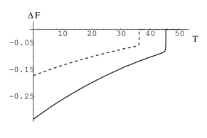
Figure 10: Free energy difference between ordered and disordered states associated to the striped (full line) and bubble (dashed line) phases for MnAs:GaAs films as a function of temperature (in Celsius degrees). The lines correspondent to the configurations for which the $y$ direction is non-modulated were removed for the sake of clearance.

V Conclusions

In this work, motivated by the recent experiments that show the morphology of the MnAs:GaAs ferromagnetic stripes, we developed a general theory that describes the magnetic phase transitions at a dipolar Ising ferromagnet slab with finite thickness and finite width. We showed that although the modulated phase occupies a smaller volume in the $(q_{x},q_{y})$ momentum space than the one occupied by the same phase in the case of an infinite slab, the transition between the ordered and the disordered configurations is still first-order and induced by fluctuations (a Brazovskii type transition). This happens because all the momentum space “shrinks” in the case of the finite slab, due to the discretization of the momentum component in the limited direction ($x$), what is a consequence of the boundary conditions. And what is fundamental to the Brazovskii transition occur is not the absolute volume of the modulated phase, but how large it is when compared to the rest of the momentum space. So, in the case we studied there is still enough phase space to the fluctuations of the order parameter induce a transition.

We also showed that, for the finite slab, there is the possibility of first-order transitions between the modulated and the disordered phases driven not by temperature, but by variation of the slab’s width. Studying two different modulated configurations, namely, striped (figure 2b) and bubble (figure 7b) ones, we showed that the first has lower energy and higher spinodal then the latter, what means that bubble phases are not expected to be observed in such materials. This is in qualitative agreement with MFM images realized on MnAs:GaAs thin films, where the domain structures inside the ferromagnetic terraces are similar to the stripes of figure 2b).

Another effect of the finiteness of the slab was that modulated phases characterized by different number of “spread” domains (referring to the semi-ellipsis minimum energy projection along the $q_{x}$ axis ) have different energies. Thus, fluctuations of the order parameter, together with finite size effects, break the high degree of degeneracy of the ground state. In the case of the infinite slab, there was already a break of degeneracy (referring to the differences in energy between striped and bubble phases, for instance), but in the finite case, we noticed that it was deeper (as some degeneracies between different stripes are also broken). It is clear that this effect, in the momentum space, is a consequence of the break of translational invariance in the real space. However, for the case of the MnAs:GaAs system studied so far, we saw that this break is practicable undetectable, due to the large film thickness (hundreds of lattice parameters) and temperature (that is far below the spinodal limit).

In addition, we noted that for slabs whose widths $d$ are “commensurate” with the modulation wavelength $\pi/q_{0}$, the most stable configuration is the one for which there is no modulation along the unlimited ($y$) direction. This is reflected by the occurrence of steps in the energy profiles of the system. In what concerns MnAs:GaAs films, we noticed that such steps generate local minima in the free energy profile that are responsible for changes of the number of “spread” domains in the $x$ direction inside the ferromagnetic terraces. Although MFM images reveal that there can be phases, inside the terraces, with different number of domains ($2$ and $3$), they show that this number is not so large as the predicted by our model (below $10$). Moreover, it was not reported yet any configuration without modulation along the $y$ direction. In fact, we do not expect that this actually happens, not only because of the precision required (the slab’s width must be commensurate to the modulation wavelength), but also for the fact that the $y$ direction is not unlimited. Rather, we expect that the mean modulation along the $y$ direction increases with temperature and oscillates near the region where the “commensurate widths” occur, as showed in figure 9. Unfortunately, as of yet there is no experiments that can verify this behaviour.

Hence, this model is only the first step towards a more complete understanding of the complex features of the MnAs:GaAs phase diagram and could be applied to other similar systems where there is a competition between organizing and frustrating interaction plus a finite slab geometry. An improved theory should surely comprehend not an Ising model, but a vectorial one, even because it is observed, in the MFM images, configurations in which the magnetization lies along the $x$ axis. Due to the crystalline field of the material, no components of the magnetization along the $y$ direction is expected. Another important thing to take into account is the topological defects, which can play fundamental role in two-dimensional systems.

Appendix A: Dipolar energy

In this appendix, we explicitly calculate the magnetostatic energy of an arbitrary configuration of the slab. First, let us derive a general expression to compute magnetostatic energies: given a certain magnetization $\vec{M}(\vec{r})$, in the absence of free currents, the magnetic field generated can be described by the magnetic scalar potential $\phi(\vec{r})$ that satisfies the Poisson equation jackson :

$$\nabla^{2}\phi=-4\pi\rho\,,$$

where $\rho$, the effective magnetic poles density, is given by:

$$\rho=-\vec{\nabla}\cdot\vec{M}\,.$$

Hence, the magnetostatic energy is written, in the Fourier space, as:

$$E=2\pi\int\frac{\left|\rho(\vec{k})\right|^{2}}{k^{2}}d^{3}k\,.$$ (49)

Let us now apply this formalism to our specific case, namely, an arbitrary magnetization of a slab with thickness $D$ and length $d$. Making use of step functions, it can be written, in the whole space, as:

$$\vec{M}(\vec{x})=M(x,y)\theta(x)\theta(d-x)\theta(D/2-z)\theta(D/2+z)\hat{z}\,,$$ (50)

where $M(x,y)$ is given by (3), as explained before. Hence, a straightforward calculation yields, for the effective magnetic poles density in the Fourier space:

$$\rho(\vec{k})=\left(\frac{g\mu_{B}}{a^{3}}\right)\frac{-iL_{y}}{(2\pi)^{3/2}}\sum_{n}m_{n,k_{y}}\sin\left(\frac{k_{z}D}{2}\right)\left[e^{ik_{x}d}(-1)^{n}-1\right]\left[\frac{1}{(k_{x}+n\pi/d)}-\frac{1}{(k_{x}-n\pi/d)}\right]\,.$$

Substituting this expression in (49), we obtain the dipolar energy:

$$E=\frac{2L_{y}^{2}}{d^{2}}\left(\frac{g\mu_{B}}{a^{3}}\right)^{2}\sum_{n,n^{\prime}}nn^{\prime}\int d^{3}k\,\frac{m_{n,k_{y}}m_{n^{\prime},-k_{y}}}{\left(k_{x}^{2}+k_{y}^{2}+k_{z}^{2}\right)}\sin^{2}\left(\frac{k_{z}D}{2}\right)\frac{\left[1+(-1)^{nn^{\prime}+1}\cos(k_{x}d)\right]}{\left(k_{x}^{2}-\frac{n^{2}\pi^{2}}{d^{2}}\right)\left(k_{x}^{2}-\frac{n^{\prime 2}\pi^{2}}{d^{2}}\right)}\,,$$

where the summation is to be understood as involving $n$ and $n^{\prime}$ with same parity. Therefore, there are three integrals to be evaluated; the one referring to $k_{y}$ can be rewritten as a summation and the one referring to $k_{z}$ can be calculated analytically:

$$\int_{-\infty}^{\infty}dk_{z}\frac{\sin^{2}\left(\frac{k_{z}D}{2}\right)}{\left(k_{x}^{2}+k_{y}^{2}+k_{z}^{2}\right)}=\frac{\pi}{2}\frac{\left(1-e^{-D\sqrt{k_{x}^{2}+k_{y}^{2}}}\right)}{\sqrt{k_{x}^{2}+k_{y}^{2}}}\,,$$

yielding the following expression for the density of dipolar energy:

$$f_{dip}=\frac{E}{L_{y}Dd}=\frac{4\pi^{2}}{Dd^{3}}\left(\frac{g\mu_{B}}{a^{3}}\right)^{2}\sum_{k_{y},n,n^{\prime}}nn^{\prime}m_{n,k_{y}}m_{n^{\prime},-k_{y}}\int_{0}^{\infty}dk_{x}\frac{\left(1-e^{-D\sqrt{k_{x}^{2}+k_{y}^{2}}}\right)\left[1+(-1)^{nn^{\prime}+1}\cos(k_{x}d)\right]}{\sqrt{k_{x}^{2}+k_{y}^{2}}\left(k_{x}^{2}-\frac{n^{2}\pi^{2}}{d^{2}}\right)\left(k_{x}^{2}-\frac{n^{\prime 2}\pi^{2}}{d^{2}}\right)}$$

which, by a simple change of coordinates, becomes expression (5).

References

- (1) M. Seul and D. Andelman, Science 267, 476 (1995)
- (2) T. Garel and S. Doniach, Phys. Rev. B 26, 325 (1982)
- (3) R. Allenspach and A. Bischof, Phys. Rev. Lett. 69, 3385 (1992)
- (4) D. Wu, D. Chandler and B. Smith, J. Phys. Chem. 96, 4077 (1992)
- (5) R. M. Weis and H. M. McConnell, Nature (London) 310, 47 (1984)
- (6) G. H. Fredrickson and E. Helfand, J. Chem. Phys. 87 (1987)
- (7) E. Brézin and J. Zinn-Justin, Nucl. Phys. B 257[FS14], 867 (1985)
- (8) S. Singh and R. K. Pathria, Phys. Pev. B 34, 2045 (1986)
- (9) A. Esser, V. Dohm and X. S. Chen, Physica A 222, 355 (1995)
- (10) J. Rudnick, G. Gaspari and V. Privman, Phys. Pev. B 32, 7594 (1985)
- (11) W. Huhn and V. Dohm, Phys. Rev. Lett. 61, 1368 (1988)
- (12) V. Dohm, Z. Phys. B - Condensed Matter 75, 109 (1989)
- (13) S. A. Brazovskii, Zh. Eksp. Teor. Fiz. 68, 175 (1975)
- (14) A. K. Das, C. Pampuch, A. Ney, T. Hesjedal, L. Däweritz, R. Koch and K. H. Ploog, Phys. Rev. Lett. 91, 087203 (2003)
- (15) M. Tanaka, Semicond. Sci. Technol. 17, 327 (2002)
- (16) C. P. Bean and D. S. Rodbell, Phys. Rev. 126, 104 (1962)
- (17) V. M. Kaganer, B. Jenichen, F. Schippan, W. Braun, L. Daweritz and K. H. Ploog, Phys. Rev. B 66, 045305 (2002)
- (18) A. Ney, T. Hesjedal, C. Pampuch, A. K. Das, L. Daweritz, R. Koch, K. H. Ploog, T. Tolinski, J. Lindner, K. Lenz and K. Baberschke, Phys. Rev. B 69, 081306 (2004)
- (19) R. Engel-Herbert, J. Mohanty, A. Ney, T. Hesjedal, L. Däweritz and K. H. Ploog, Appl. Phys. Lett. 84, 1132, 2004.
- (20) R. Magalhães-Paniago, L. N. Coelho, B. R. A. Neves, H. Westfahl, F. Iikawa, L. Daweritz, C. Spezzani and M. Sacchi, Appl. Phys. Lett. 86, 053112 (2005)
- (21) F. Iikawa, M. Knobel, P. V. Santos, C. Adriano, O. D. D. Couto, M. J. S. P. Brasil, C. Giles, R. Magalhães-Paniago and L. Daweritz, Phys. Rev. B 71, 045319 (2005)
- (22) J. W. Negele and H. Orland, Quantum Many-Particle Systems, Advanced Book Classics, Perseus, USA (1998)
- (23) P. M. Chaikin and T. C. Lubensky, Principles of Condensed Matter Physics, Cambridge University Press, United Kingdom (1995)
- (24) A. Kashuba and V. L. Pokrovsky, Phys. Rev. Lett. 70, 3155 (1993)
- (25) R. M. Fernandes, H. Westfahl Jr., R. Magalhães-Paniago and L. N. Coelho, cond-mat/0605357 (2006)
- (26) T. Plake, T. Hesjedal, J. Mohanty, M. Kastner, L. Däweritz and K. H. Ploog, Appl. Phys. Lett. 84, 1132 (2004)
- (27) L. N. Coelho, R. Magalhães-Paniago, B. R. A. Neves, F. C. Vicentin, H. Westfahl, R. M. Fernandes, F. Iikawa, L. Däweritz, C. Spezzani and M. Sacchi, cond-mat/0605356 (2006)
- (28) J. D. Jackson, Classical Electrodynamics, John Wiley and Sons, USA (1998)