The quenching of compressible edge states around antidots

Abstract

We provide a systematic quantitative description of the edge state structure around a quantum antidot in the integer quantum Hall regime. The calculations for spinless electrons within the Hartree approximation reveal that the widely used Chklovskii et al. electrostatic description greatly overestimates the widths of the compressible strips; the difference between these approaches diminishes as the size of the antidot increases. By including spin effects within density functional theory in the local spin-density approximation, we demonstrate that the exchange interaction can suppress the formation of compressible strips and lead to a spatial separation between the spin-up and spin-down states. As the magnetic field increases, the outermost compressible strip, related to spin-down states starts to form. However, in striking contrast to quantum wires, the innermost compressible strip (due to spin-up states) never develops for antidots.

A quantum antidot is a potential hill in a two-dimensional electron gas (2DEG) usually defined by means of an electrostatic split gate, see Fig. 1. In a perpendicular magnetic field, electrons are trapped around the antidot in bound states formed by magnetic confinement. Experimental studies of magnetotransport in quantum antidots reported over the last decade reveal a rich magneto-conductance structure in the quantum Hall regime Andy ; Goldman_Science ; Maasilta ; Karakurt ; Goldman2005 ; Ford_1994 ; Mace ; Kataoka_1999 ; Kataoka_2000 ; Kataoka_2002 ; Kataoka_2003 . Some of the observed magneto-conductance features can be understood within a one-electron picture in terms of semi-classical and quantum electron dynamics Andy . However, a majority of experiments confirm a central role played by electron interactions and spin effects in antidot measurements. This includes, for example, the first direct observation of the fractionally quantized electron charge Goldman_Science , fractional statistics Goldman2005 , the striking effect of the frequency doubling of the Aharonov-Bohm (AB) oscillations Ford_1994 ; Kataoka_2000 , the detection of the Coulomb charging Kataoka_1999 , the observation of the Kondo effect Kataoka_2002 and selective spin-injection Kataoka_2003 . Interest in antidot structures is also motivated by their potential for spintronic applications, where they can be used to inject or detect spin-polarized currents APL or even as quantum gates Berggren . The antidots also provide a system for investigating edge states in general, because of the detailed information one can obtain from the dependence of AB peak positions on field and gate voltage.

A detailed microscopic understanding of antidot systems therefore requires a rigorous theory accounting for both interaction and spin effects. In contrast to quantum dots and wires which have been the subject of intense theoretical study (see e.g. QDOverview ; Ihnatsenka and references therein), the energetics of quantum antidots has received, with only a few exceptions Hwang , practically no attention. In particular, the central issue concerning the structure of edge states and the formation of the compressible strips around antidots still remains an open question. The structure of the antidot edge states represents an important key to an understanding of various effects such as AB oscillations Ford_1994 ; Kataoka_2000 , Coulomb charging Kataoka_1999 and spin selectivity Kataoka_2003 , and it has been a subject of recent lively discussions Karakurt ; PRL_comments . The main goal of the present paper is to provide a rigorous theoretical description for the spin-resolved structure of edge states around a quantum antidot.

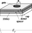
Figure 1: Calculated electrostatic confinement potentials $V_{conf}(r)$ for a quantum antidot with different gate radii $R$. The inset shows a schematical layout of the device defined in GaAs heterostructure with a cap layer of the width $c=14$ nm, a donor layer of the width $d=36$ nm, and a spacer layer of the width $s=10$ nm. The donor concentration $n_{d}=6\cdot 10^{23}$ m^-3. The above parameters (corresponding to the bulk electron density $n_{bulk}\sim 2\cdot 10^{15}\text{m}^{-2}$) are used for all antidot structures discussed in the paper.

We consider an antidot defined within a GaAs heterostructure by a circular gate of radius $R$ as illustrated in the inset to Fig. 1. We assume that electron motion is confined to the plane parallel to the heterostructure interface, $\mathbf{r}=(x,y).$ The external electrostatic confinement, $V_{conf}(r)=V_{Schottky}+V_{d}+V_{g}(r),$ includes the Schottky barrier $V_{Schottky}=0.8$ eV and the potential due to a layer of donors of width $d$ situated at a distance $c$ from the surface Martorell , $V_{d}=-n_{d}d\left(c+d/2\right)e^{2}/\varepsilon_{0}\varepsilon_{r},$ with $n_{d}$ being the donor concentration and $\varepsilon_{r}$ the GaAs dielectric constant. The electrostatic potential $V_{g}(r)$ due to a circular gate is given by an analytical expression provided by Davies (Eq. (3.17) in Ref. Davies, ). The electrostatic confinement $V_{conf}(r)$ for different gate radii $R$ is shown in Fig. 1 .

Utilizing the circular symmetry of the structure we introduce cylindrical coordinates and write down the wave function in the form $\psi(r)=e^{il\varphi}\phi(r),$ where $l=0,\pm 1,\ldots$ is the orbital quantum number. The Schrödinger equation in a perpendicular magnetic field $B$ reads

$$-\frac{1}{r}\frac{\partial}{\partial r}r\frac{\partial\phi^{\sigma}(r)}{\partial r}+\left[\left(\frac{l}{r}+\frac{qr}{2}\right)^{2}+V^{\sigma}(r)\right]\phi^{\sigma}(r)=E\phi^{\sigma}(r),$$ (1)

where the lengths are measured in units of the lattice constant $a$ (used for numerical discretization), energies in units of $\hbar^{2}/2m^{\ast}a^{2};$ $q=eBa^{2}/\hbar,$ and $\sigma=\pm{\frac{1}{2}}$ describes spin-up and spin-down states, $\uparrow,\downarrow$. We include electron interactions and spin effects within the framework of density functional theory (DFT) in the local spin density approximation (LSDA) ParrYang . The choice of DFT+LSDA for the description of many-electron effects is motivated, on one hand, by its practical implementation efficiency within a standard Kohn-Sham formalism Kohn , and on the other hand, by the excellent agreement between the DFT+LSDA and exact diagonalization Stephanie and variational Monte-Carlo calculations Rasanen ; QDOverview performed for few-electron systems. Within the framework of the DFT+LSDA, the total confinement potential can be written in the form

$$V^{\sigma}(r)=V_{conf}(r)+V_{H}(r)+V_{xc}^{\sigma}(r)+g\mu_{B}B\sigma,$$ (2)

where

$$V_{H}(r)=\frac{e^{2}}{4\pi\varepsilon_{0}\varepsilon_{r}}\int d\mathbf{r}^{\prime}n(\mathbf{r}^{\prime})\left[\frac{1}{\left|\mathbf{r}-\mathbf{r}^{\prime}\right|}-\frac{1}{\sqrt{\left(\mathbf{r}-\mathbf{r}^{\prime}\right)^{2}+4b^{2}}}\right]$$ (3)

is the Hartree potential including the contribution from mirror charges ($b$ is the distance from the 2DEG to the surface), $n(r)=\sum_{\sigma}n^{\sigma}(r);\;n^{\sigma}(r)=\sum_{i}\left|\psi_{i}^{\sigma}(r)\right|^{2}f_{FD}(E-E_{F})$ is the electron density, and $f_{FD}$ is the Fermi-Dirac distribution. For the exchange and correlation potential $V_{xc}^{\sigma}(r)$ we utilize a widely used parameterization from Tanatar and Cerperly TC (see Ref. Ihnatsenka, for the explicit expressions for $V_{xc}(r)$). This parameterization is valid for magnetic fields corresponding to filling factors $\nu>1$, which sets the limit for the applicability of our results. The last term in Eq. (2) accounts for the Zeeman energy where $\mu_{b}=\frac{e\hbar}{2m_{e}}$ is the Bohr magnetron, and the bulk $g$ factor of GaAs is $g=-0.44$. We solve Eq. (1) self-consistently expanding the wavefunctions into sin-basis. Because the antidot represents an open system, we choose the computational domain sufficiently large to ensure that the electron density in the bulk (i.e. far away from the antidot) is constant and does not change when we increase the domain size.

Following our previous analysis of edge state structure in quantum wires Ihnatsenka ; Ihnatsenka2 ; Ihnatsenka3 , we start with the Hartree approximation [disregarding exchange and correlation interactions by setting $V_{xc}^{\sigma}(r)=0$ in Eq. (2) ]. Figure 2 (a) shows the electron density profiles (the local filling factors) $\nu(r)=n(r)/n_{B}$ $(n_{B}=eB/h)$ around antidots with different radii for a representative value of magnetic field $B=4.2$ T. The corresponding average wave function positions $\psi_{i}$ for different eigenenergies $E_{i}$ (i.e. the magnetosubbands) are shown in Figs. 2 (b)-(d) illustrating the formation of the compressible strips around the antidots. [Note that in Fig. 2 each eigenstate $\psi_{i}$ is represented by a dot. Because of a large number of the eigenstates, $\sim 10^{4},$ the dots are merged into solid lines]. The compressible strips are composed of partially filled electron states that screen the external potential and lead to a flattening of the subbands in the compressible regions Chklovskii . [Following Refs. Ando ; Ihnatsenka ; Ihnatsenka2 ; Ihnatsenka3 We define the compressible strips within the window $\left|E-E_{F}<2\pi kT\right|$)]. Figure 2 also shows the total confining potential $V(r)$, Eq. (2). Note that the calculated spin-up and spin-down densities and potentials are virtually indistinguishable on the scale of the figure. Hence, in this magnetic field interval the effect of the Zeeman term on the subband structure is negligible, so that we may refer to the Hartree results as being the case of spinless electrons.

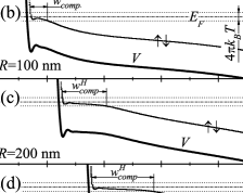
Figure 2: (a) The electron density profile (local filling factor), $\nu(r)=n(r)/n_{B}$ for antidots of different radii $R$ calculated in the Hartree approximation. (b) The corresponding magnetosubband structure (i.e. the overage position of the wave functions $\psi_{i}$). Fat solid lines indicate the total confining potential $V(r)$, Eq. (2). Magnetic field $B=4.2$ T. Temperature $T=1$ K.

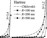
Figure 3: Width of the compressible strips around quantum antidot with different radii $R$ as a function of magnetic field calculated within the Hartree approximation (i.e. for the spinless electrons) and its comparison to the Chklovskii et al. predictions Chklovskii . $N=1,2$ and 3,4 refer to the subband number corresponding to the two lowest (spin degenerate) edge states. Temperature $T=1$ K.

Figure 3 shows the width of the compressible strips for spinless electrons, $w_{comp}^{H}$, around antidots of different radii. For a comparison, we also plot Chklovskii et al. Chklovskii analytical expressions, $w_{comp}^{Chk},$ giving the length of the compressible strips at the edge of a semi-infinite 2DEG. [$w_{comp}^{Chk}$ depends on two parameters, the depletion length $l,$ and the filling factor in the bulk, $\nu_{bulk}=n_{bulk}/n_{B}.$ We extract $l$ from the calculated self-consistent density distribution by fitting to the dependence $n(r)=n_{bulk}\left(\frac{r-l}{r+l}\right)^{1/2}$where $n_{bulk}$ is the electron density far away from the antidot Chklovskii ; Ando ; Ihnatsenka2 ]. It has been demonstrated that for the case of quantum wires the width of the compressible strips for spinless electrons calculated in the Hartree approach, $w_{comp}^{H},$ is in very good agreement with the Chklovskii et al. predictions Chklovskii for $w_{comp}^{Chk}$ Ando ; Ihnatsenka2 . This is obviously not the case for the antidot structures where the Chklovskii et al. predictions Chklovskii greatly overestimates the compressible strip width. For example, for an antidot with the radius $R=200$ nm, the innermost compressible strip (i.e. corresponding to the edge state closest to the antidot) starts to form at $B\approx 3.9$ T, whereas for the 2DEG edge this strip starts to already form at $B\approx 2.6$ T, see Fig. 3. The difference between $w_{comp}^{H}$ and $w_{comp}^{Chk}$ is most pronounced for small antidot radii $R$ and decreases as $R$ increases (note that the limit $R\rightarrow\infty$ effectively corresponds to the case of a straight boundary, i.e. the semi-infinite 2DEG). The difference between $w_{comp}^{H}$ and $w_{comp}^{Chk}$ can be understood as follows. For the case of a semi-infinite gate an electron in the vicinity of the edge of the 2DEG experiences the Hartree potential originated from electrons in the semi-infinite region not covered by the gate. However, for the case of the antidot the Hartree potential is stronger as it includes an additional contribution from the electrons surrounding the antidot (that are otherwise depleted for the case of the semi-infinite 2DEG). This additional contribution effectively repels the electrons from the boundary towards the bulk of the 2DEG. This leads to less effective screening and thus to steeper potential preventing the formation of compressible strips.

Figure 4: (Color online) (a) Width of the compressible strips for spinless electrons in the Hartree approximation, $w_{comp}^{H}$, as compared to $d_{sep}+w_{comp}^{\downarrow DFT}$ calculated within DFT. (b) With of the compressible strips for spin-up and spin-down states $w_{comp}^{\uparrow DFT},w_{comp}^{\downarrow DFT}$ calculated within DFT. (c), (e) The electron density profiles (local filling factor), $\nu^{\sigma}(r)=n^{\sigma}(y)/n_{B}$ for different magnetic fields (indicated by arrows in (a)) $B=4.3$ T and $4.4$ T, and, (d), (f) the corresponding magnetosubband structure (i.e. the overage position of the wave functions $\psi^{\sigma}_{i}$). Fat solid lines indicate the total confining potential $V^{\sigma}(r)$ , Eq. (2). $T=1$ K.

Let us now analyze the spin-resolved edge state structure within the DFT approximation. Figures 4 (c)-(f) show the electron density profiles (the local filling factors) $\nu^{\sigma}(r)=n^{\sigma}(r)/n_{B}$ and the average wave function position $\psi_{i}^{\sigma}$ for different energies $E_{i}^{\sigma}$ (the magnetosubband structure) around the antidots with radius $R=200$ nm for different representative magnetic fields $B=4.3$ T and $B=4.4$ T. Within the Hartree approximation the subbands are virtually degenerate since the Zeeman splitting is very small in the magnetic field interval under investigation (see Fig. 2). In contrast, the exchange interaction included within the DFT approximation causes the separation of the subbands for spin-up and spin-down electrons. Indeed, the exchange potential for spin-up electrons depends on the density of spin-down electrons and vice versa ParrYang ; TC ; Ihnatsenka . In compressible regions the subbands are only partially filled (because $f_{FD}<1$ in the the window $|E-E_{F}|\lesssim 2\pi kT$), and, therefore, the population of spin-up and spin-down subbands may be different. In the DFT calculation, this population difference (triggered by Zeeman splitting) is strongly enhanced by the exchange interaction leading to different effective potentials for spin-up and spin-down electrons and eventually to a subband spin splitting. As a result, the compressible region present in the Hartree approximation is suppressed and the spin-up and spin-down states become spatially separated by the distance $d_{sep}\approx w_{comp}^{H}$, see Figs. 4 (a)-(d). On further increasing the magnetic field the compressible strip starts to form for the outer (spin-down) state such that $d_{sep}+w_{comp}^{\downarrow DFT}\approx w_{comp}^{H},$ see Figs. 4 (a)–(b),(e)-(f) ($w_{comp}^{\sigma DFT}$ is the width of the compressible strip for the spin state $\sigma$ calculated in the DFT approximation).

Far away from the antidot the subbands remain degenerate since they are situated below the Fermi energy $E\lesssim E_{F}-2\pi kT$ and are thus fully occupied ($f_{FD}=1$). As a result, the corresponding spin-up and spin-down densities are the same, hence the exchange and correlation potentials for the spin-up and spin-down electrons are equal, $V_{xc}^{\uparrow}(r)=V_{xc}^{\downarrow}(r)$.

A similar scenario for subband spin splitting also holds for quantum wires Ihnatsenka2 . However, an important and interesting distinction is that for quantum wires, as the magnetic field is increased, compressible strips form first for spin-up and then for spin-down states. In contrast, for the case of the antidot only the compressible strip for the spin-down state forms, whereas the compressible strip for the spin-up states (situated close to the antidot) never develops, see Fig. 4(b) [This conclusion holds for all antidots sizes studied in this paper, see Fig. 1]. Just as for the case of spinless electrons discussed above, we attribute this difference to less effective screening for the antidot structure leading to a rather steep potential near the antidot boundary that prevents formation of the compressible strip for the innermost (spin-up) state. Note that the absence of the compressible strip for the inner (spin-up) state is consistent with the interpretation of the unexpected doubling of the frequency of the Aharonov-Bohm oscillations explained in Ref. Kataoka_2000 in terms of a charging of the outermost compressible regions around the antidots by electrons of the same spin. Our calculations indicate that the charging of the innermost (spin-up states) is unlikely since the spin-up states do not form the compressible regions. [We note however, that we are not yet in a position to comment on whether charging of the compressible strips proposed in Ref. Kataoka_2000 really does takes place. The answer to this question can be obtained from self-consistent transport calculations similar to those reported in e.g. Ref. open_dot . Such calculations are currently in progress.]

Finally we stress that all the results and conclusions presented in this paper for a temperature $T=1$ K remain valid for lower temperatures, since calculations performed for $T=0.2$ K reveal that the width of the compressible strips remain practically unchanged.

It is important to note that the effect of reduced screening that strongly affects the antidot edge structure as discussed above might also be imperative for the case of quantum dot, where the spin selectivity in the edge state regime might strongly depend on the gate layout Ciorda . The implications of this effect for quantum dot geometries remains to be identified.

To conclude, we find that for spinless electrons edge states around an antidot start to form for magnetic fields significantly higher than those predicted by Chklovskii et al. electrostatic description Chklovskii . By including spin effects within spin density functional theory we show that the exchange interaction leads to qualitatively novel features in antidot edge state structure, such as the suppression of compressible strips for lower fields, spatial separation between spin-up and spin down states, and to the total absence of the innermost compressible strip due to spin-up states (as opposed to the outermost compressible strip due to spin-down states that forms at higher fields).

S. I. acknowledges financial support from the Swedish Institute. Discussions with C. J. B. Ford, M. Kataoka and A. S. Sachrajda are greatly appreciated. We thankful to C. J. B. Ford and A. S. Sachrajda for critical reading of the manuscript and valuable suggestions.

References

- (1) G. Kirczenow et al., Phys. Rev. Lett. 72, 2069 (1994); C. Gould, et al., ibid., 77, 5272 (1996).
- (2) V. J. Goldman and B. Su, Science 267, 1010 (1995).
- (3) I. J. Maasilta and V. J. Goldman, Phys. Rev. B 57 R4273 (1998).
- (4) I. Karakurt et al., Phys. Rev. Lett. 87, 146801 (2001).
- (5) V. J. Goldman, J. Liu and A. Zaslavsky, Phys. Rev. B 71, 153303 (2005).
- (6) C. J. B. Ford et al., Phys. Rev. B 49, 17456 (1994).
- (7) D. R. Mace et al., Phys. Rev. B 52, R8672 (1995).
- (8) M. Kataoka et al., Phys. Rev. Lett 83, 160 (1999).
- (9) M. Kataoka et al., Phys. Rev. B 62, R4817 (2000).
- (10) M. Kataoka et al., Phys. Rev. Lett 89, 226803 (2002).
- (11) M. Kataoka et al., Phys. Rev. B 68 153305 (2003).
- (12) I. V. Zozoulenko and M. Evaldsson, Appl. Phys. Lett. 85, 3136 (2004).
- (13) P. Jaksch, I. Yakimenko, K.-F. Berggren, Intl. J. of Nanoscience 3, 309 (2004).
- (14) S. M. Reimann and M. Manninen, Rev. Mod. Phys. 74, 1283 (2002).
- (15) S. Ihnatsenka and I. V. Zozoulenko, Phys. Rev. B 73, 075331 (2006).
- (16) N. Y. Hwang, et al., Phys. Rev. B 70, 085322 (2004).
- (17) M. Kataoka and C. J. B. Ford, Phys. Rev. Lett. 92, 199703 (2004); V. J. Goldman, ibid., 199704 (2004).
- (18) J. Martorell, H. Wu and D. W. L. Sprung, Phys. Rev. B 50, 17298 (1994).
- (19) J. H. Davies, Semicond. Sci. Techn. 3, 995 (1988).
- (20) R. G. Parr and W. Yang, Density-Functional Theory of Atoms and Molecules, (Oxford Science Publications, Oxford, 1989).
- (21) W. Kohn and L. Sham, Phys. Rev. 140, A1133 (1965).
- (22) M. Borgh et al., Intl. J. Quant. Chem. 105, 817 (2005).
- (23) E. Räsänen et al., Phys. Rev B 67, 235307 (2003).
- (24) B. Tanatar and D. M. Ceperley, Phys. Rev. B 39, 5005, (1989).
- (25) S. Ihnatsenka and I. V. Zozoulenko, Phys. Rev. B 73, 155314 (2006).
- (26) S. Ihnatsenka and I. V. Zozoulenko, Phys. Rev. B, to be published (cond-mat/0605008).
- (27) D. B. Chklovskii, B. I. Shklovskii, and L. I. Glazman, Phys. Rev. B 46, 4026 (1992); D. B. Chklovskii, K. A. Matveev, and B. I. Shklovskii, Phys. Rev. B 47, 12605 (1993).
- (28) T. Suzuki and T. Ando, Physica B 249-251, 415 (1998).
- (29) M. Evaldsson and I. V. Zozoulenko, Phys. Rev. B 73, 035319 (2006).
- (30) M. Ciorga et al., Phys. Rev. B. 61, R16315 (2000).