Power-law random walks

Abstract

We present some new results about the distribution of a random walk whose independent steps follow a $q-$Gaussian distribution with exponent $\frac{1}{1-q};\,\,\,q\in\mathbb{R}$. In the case $q>1$ we show that a stochastic representation of the point reached after $n$ steps of the walk can be expressed explicitly for all $n$. In the case $q<1,$ we show that the random walk can be interpreted as a projection of an isotropic random walk, i.e. a random walk with fixed length steps and uniformly distributed directions.

I Introduction

The name “random walk" (RW) was originally proposed by Pearson in 1901 pearson with reference to a simple model to describe mosquito infestation in a forest, although previous important work in related subjects had been already published by Lord Rayleigh. Around the same time, the theory of random walks was also developed by Bachelier in a remarkable doctoral thesis published in 1900 pearson . He proposed the random walk as the fundamental model for financial time series, long before this idea became the basis for modern theoretical finance. He also made the connection between discrete random walks and the continuous diffusion (or heat) equation, which is a major scientific theme. Around the same time as Pearson’ s work, Einstein also published his seminal paper on Brownian motion (normal diffusion), a random walk driven by collisions with gas molecules. Similar theoretical ideas were also published independently by Smoluchowski pearson . One can confidently assert that RW is one of the most basic themes of science.

The statistical properties of random walks tend toward universal distributions after large numbers of independent steps. In the case of the concomitant probability distribution function (PDF) for the final position, the result for isotropic random walks is a multidimensional generalization of the Central Limit Theorem (CLT) for sums of independent, identically distributed (IID) random variables. When the assumptions of the Central Limit Theorem break down, random walks can exhibit rather different behavior from that of normal diffusion. For instance, the limiting distribution for the position of a Brownian particle may not be Gaussian. In particular, power-law distributions become of paramount importance in such a context. One way to violate the CLT with IID displacements is via “heavy-tailed" probability distributions, which assign sufficient probability to very large steps so that the variance is infinite. In this context one speaks of anomalous diffusion (AD). In an AD-scenario power-law probability distributions and power-law entropies become ubiquitous. The associated literature is really vast. See for instance, Ref. okamoto ; gellmann ; lissia ; euro ; anteneodo and references therein.

In this effort we revisit the distribution of a random walk whose independent steps follow a power-law distribution of the $q-$Gaussian type with exponent equal to $1/(1-q);\,\,\,q\in\mathbb{R}.$ In the case $q>1$ we show that a stochastic representation of the point reached after $n$ steps of the walk can be expressed explicitly for all $n$ so that the superstatistics framework holds even in the anomalous diffusion case. In the case $q<1,$ we show that the $q-$Gaussian random walk can be interpreted as a projection of an isotropic random walk, i.e. a random walk with fixed length steps and uniformly distributed directions.

II The case $q>1$

A random vector $X\in\mathbb{R}^{p}$ is of the q-Gaussian kind if its probability density is

$$f_{X}\left(X\right)=Z_{q}^{-1}\left(1+X^{t}\Lambda^{-1}X\right)^{\frac{1}{1-q}}$$ (II.1)

where the number of degrees of freedom $m$, dimension $p$ and non-extensivity parameter $q$ are related as

$$m=\frac{2}{q-1}-p,$$ (II.2)

This distribution has finite covariance matrix $K=EXX^{t}$ provided that $m>2$ or equivalently $q<\frac{p+4}{p+2}.$ In that case, the covariance matrix is related to the scaling matrix $\Lambda$ in the fashion

$$\Lambda=\left(m-2\right)K.$$ (II.3)

Moreover, the partition function $Z_{q}$ reads

$$Z_{q}=\left(\frac{\Gamma\left(\frac{1}{q-1}\right)}{\Gamma\left(\frac{1}{q-1}-\frac{p}{2}\right)|\pi\Lambda|^{1/2}}\right)^{-1}.$$

Note that the usual Gaussian distribution corresponds to the limit case $q\rightarrow 1^{+}.$ We recall 3NC ; vignat ; plastino that random vector $X$ can be expressed as the Gaussian scale mixture

$$X=\frac{\Lambda^{1/2}G}{\sqrt{a}}$$ (II.4)

where $G$ is a $p-$variate, unit covariance Gaussian random vector and $a$ is a random variable independent of $G$ that follows a $\chi^{2}$ distribution with $m$ degrees of freedom. Representation (II.4) reflects exactly the notion of superstatistics as introduced by Beck and Cohen B1 ; B2 ; B3 ; B4 ; B5 ; B6 ; B7 : a $q-$Gaussian random system with $q>1$ can be interpreted as a Gaussian system submitted to multiplicative fluctuations following an inverse chi distribution.

II.0.1 the finite covariance case

In the context of a random walk, we are interested in the distribution of the normalized random vector

$$Z_{n}=\frac{1}{\sqrt{n}}\sum_{i=1}^{n}X_{i}$$ (II.5)

where random vectors $X_{i}\in\mathbb{R}^{p}$ are independent and q-Gaussian distributed according to (II.1), each with $m$ degrees of freedom and covariance matrix $K.$ Random vector $Z_{n}$ can be characterized by the following

Theorem 1

A stochastic representation of random vector $Z_{n}$ is

$$Z_{n}\sim\alpha_{m,n}\left(\sum_{i=1}^{n}\frac{1}{\nu_{i}}\right)^{\frac{1}{2}}X$$ (II.6)

where the $p-$variate vector $X$ is q-Gaussian distributed with $nm$ degrees of freedom and covariance matrix $K,$ where the constant quantity $\alpha_{m,n}=\frac{1}{n}\sqrt{\frac{m-2}{m-\frac{2}{n}}}$, while $\left\{\nu_{1},\dots,\nu_{n-1}\right\}$ are Dirichlet distributed with parameters $m_{1}=\dots=m_{n}=m$ and independent of vector $X$.

Proof: We follow here the proof given in Dickey : a linear combination of Gaussian scale mixtures is itself a Gaussian scale mixture since symbol

$$Z_{n}=\frac{1}{\sqrt{n}}\sum_{i=1}^{n}\frac{\Lambda^{1/2}G_{i}}{\sqrt{a_{i}}}$$ (II.7)

$$\sim\frac{1}{\sqrt{n}}\sqrt{\sum_{i=1}^{n}\frac{1}{a_{i}}}\Lambda^{1/2}G$$ (II.8)

$$=\frac{1}{\sqrt{n}}\sqrt{\sum_{i=1}^{n}\frac{\sum_{j=1}^{n}a_{j}}{a_{i}}}\frac{\Lambda^{1/2}G}{\sqrt{\sum_{j=1}^{n}a_{j}}}$$ (II.9)

where $G$ is a $p-$variate Gaussian vector with unit covariance. Now we remark that random variables $a_{i}$ are chi-square distributed with $m$ degrees of freedom; thus, by Luckacs’ result, each random variable

$$\nu_{i}=\frac{a_{i}}{\sum_{j=1}^{n}a_{j}}$$ (II.10)

is independent of $\sum_{j=1}^{n}a_{j}.$ Moreover, equality (II.10) shows that random variables $\left\{\nu_{i}\right\}_{1\leq i\leq n-1}$ are Dirichlet distributed. At last, since $\sum_{j=1}^{n}a_{j}$ is chi-square distributed with $mn$ degrees of freedom, we deduce that

$$\frac{\sqrt{nm-2}}{\sqrt{m-2}}\frac{\Lambda^{1/2}G}{\sqrt{\sum_{j=1}^{n}a_{j}}}$$

is a $q-$Gaussian vector with covariance matrix $K$ and $mn$ degrees of freedom.  $\square$

A striking result is thus obtained: at its $n-$th step, a q-Gaussian random walk with $q>1$ is a scale mixture of a q-Gaussian vector. We note that this property holds true for any random walk with independent steps following a Gaussian scale mixture. The fact that this property extends to q-Gaussian distributions is indeed remarkable. As described in the preceding proof, this special behavior is a consequence of a famous result by Lukacs lukacs about the Gamma distributions, which are precisely the ones that rule the fluctuations described by the superstatistics theory B1 ; B2 ; B3 ; B4 ; B5 ; B6 ; B7 .
Moreover, the non-extensivity parameter $q^{\prime}$ of vector $X$ in (II.6) is related to the parameter $q$ of each step as

$$q^{\prime}=1+\frac{2(q-1)}{2+m(n-1)(q-1)}.$$ (II.11)

We note that the dimension $p$ of the random walk does not appear in this formula.

The curves in Figure 1 represent $q^{\prime}$ as a function of $n$ for

1. $m=5$ and $q=5,3$ and $1.5$ (top to bottom) on the three top curves;

2. for $m=10$ and $q=5,3$ and $1.5$ (top to bottom) on the three middle curves;

3. for $m=30$ and $q=5,3$ and $1.5$ (top to bottom) on the three lower curves.

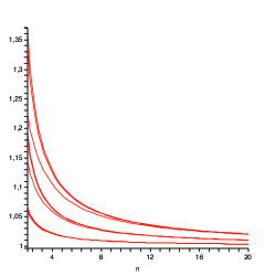
Figure II.1: $q^{\prime}$ as a function of $n$ for $m=5$ and $q=5,3$ and $1.5$ (top to bottom) on the three top curves; for $m=10$ and $q=5,3$ and $1.5$ (top to bottom) on the three middle curves; for $m=30$ and $q=5,3$ and $1.5$ (top to bottom) on the three lower curves

These curves confirm the three following results:

1. since the variance is finite, the central limit theorem applies and $Z_{n}$ converges to a Gaussian vector with covariance matrix $K$, and thus $q^{\prime}$ converges to $1$

2. the convergence to a Gaussian vector is all the faster since the number of degrees of freedom $m$ is large - or equivalently, since the independent steps $X_{i}$ are closer to Gaussian steps

3. for a large enough value of $m$, the convergence process of $q^{\prime}$ to $1$ is relatively insensitive to the value of $q.$

Unfortunately, the probability density for the scaling random variable

$$U_{m,n}=\alpha_{m,n}\left(\sum_{i=1}^{n}\frac{1}{\nu_{i}}\right)^{\frac{1}{2}},$$ (II.12)

can not be explicitly given. Figures 2 and 3 below depict an estimation of the probability distribution function for $U_{m,n}$ after $n=5,10,15,20$ and $30$ steps of the random walk in the cases $m=5$ and $m=25$. Note that different scales have been employed. These figures clearly exhibit the convergence of the random variable $U_{m,n}$ to the deterministic unit-constant, as required by the central limit theorem.

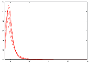
Figure II.2: estimated pdf of $U_{5,n}$ with $n=5,10,15,20$ and $30$ (bottom to top)

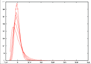
Figure II.3: estimated pdf of $U_{25,n}$ with $n=5,10,15,20$ and $30$ (bottom to top)

II.0.2 The infinite covariance case: Lévy flights

Let us assume now $m<2$ so that each of the steps of the random walk has infinite covariance. Let us consider the unnormalized random walk

$$Z_{n}=\sum_{i=1}^{n}X_{i}$$ (II.13)

The distribution of any component $X_{i}^{(k)}$ of vector $X_{i}$,

$$f_{x}(x)=\frac{\Gamma(\frac{m+1}{2})}{\Gamma(\frac{m}{2})\sqrt{\pi\Lambda_{k,k}}}(1+\frac{x^{2}}{\Lambda_{k,k}})^{-\frac{m+1}{2}}$$

behaves as

$$f_{x}(x)\sim|x|^{-m-1},\,\,|x|\sim\infty$$ (II.14)

so that the number of degrees of freedom $m$, for $m\leq 2$, coincides with the Lévy index of the $q-$Gaussian distribution. Now, by direct application of the Lévy-Gnedenko central limit theorem (gnedenko ; milan ) one immediately realizes that

$$\frac{1}{n^{1/m}}\Lambda^{-1/2}Z_{n}\Rightarrow S_{m},$$ (II.15)

where $S_{m}$ denotes a vector, each components of which follows a symmetric alpha-stable distribution with Lévy index $m$.

A quite interesting result worth quoting at this point is that, although the involved variables have infinite covariance, the superstatistics principle still applies in the following fashion:

Theorem 2

For all $n,$ the normalized random walk $\frac{1}{n^{1/m}}Z_{n}$ is distributed as a Gaussian scale mixture. Further, the distribution of the mixing variable converges, as $n\rightarrow+\infty$, to a stable distribution with Lévy index $m/2$.

Proof: We use the first part of the proof of Th. 1:

$$Z_{n}=\sum_{i=1}^{n}\frac{\Lambda^{1/2}G_{i}}{\sqrt{a_{i}}}\sim\sqrt{\sum_{i=1}^{n}\frac{1}{a_{i}}}\Lambda^{1/2}G$$ (II.16)

One can easily check that each random variable $\frac{1}{a_{i}}$ has Lévy index $m/2$. Now, the Lévy-Gnedenko theorem yields

$$\frac{1}{n^{2/m}}\sum_{i=1}^{n}\frac{1}{a_{i}}\Rightarrow S_{m/2},$$

so that

$$\frac{1}{n^{1/m}}Z_{n}\Rightarrow\sqrt{S_{m/2}}\Lambda^{1/2}G.$$

$\square$
Note that this result is coherent with the representation (II.15) as given by the Lévy Gnedenko theorem. Indeed, according to a classical result about stable random variables (see feller ), if $S_{\alpha}$ and $S_{\alpha^{\prime}}$ denote two independent stable random variables with respective indices $\alpha$ and $\alpha^{\prime}$ then,

$$S_{\alpha}S_{\alpha^{\prime}}^{1/\alpha}\sim S_{\alpha^{\prime\prime}}$$

with $\alpha^{\prime\prime}=\alpha\alpha^{\prime}$. In the above situation, this result applies component-wise with $\alpha=2$ and $\alpha^{\prime}=m/2.$

III Case $q<1$

The $p-$variate $q-$Gaussian distribution in the case $q<1$ writes explicitly as

$$f_{X}\left(X\right)=Z_{q}^{-1}\left(1-X^{t}\Lambda^{-1}X\right)_{+}^{\frac{1}{1-q}}$$ (III.1)

with notation $\left(x\right)_{+}=\max\left(x,0\right).$ The covariance matrix of vector $X$ is finite and writes $K=EXX^{t}=d^{-1}\Lambda$ with $d=p+2\frac{2-q}{1-q}$. Moreover, the partition function $Z_{q}$ writes

$$Z_{q}=\left(\frac{\Gamma\left(\frac{2-q}{1-q}+\frac{p}{2}\right)}{\Gamma\left(\frac{2-q}{1-q}\right)|\pi\Lambda|^{1/2}}\right)^{-1}.$$ (III.2)

A stochastic representation of a vector $X$ following this distribution is

$$X=\frac{\Lambda^{1/2}G}{\sqrt{G^{t}G+b}},$$ (III.3)

where the random variable $b$ is hi-square distributed with $2\frac{2-q}{1-q}$ degrees of freedom and independent of the $p-$variate, unit variance Gaussian vector $G$ and c. Let us consider now the random walk

$$Z_{n}=\frac{1}{\sqrt{n}}\sum_{i=1}^{n}X_{i},$$ (III.4)

where the random vectors $X_{i}$ are independent and follow distribution (III.1).

Although, contrarily to the case $q>1$, no explicit stochastic representation can be provided for (III.4), this kind of random walk can be given an interesting interpretation, as follows:

Theorem 3

If $Y_{n}$ is an isotropic $d-$dimensional random walk pearson

$$Y_{n}=\frac{1}{\sqrt{n}}\sum_{i=1}^{n}T_{i}$$

where $T_{i}\in\mathbb{R}^{d}$ are independent random vectors with unit length $\|T_{i}\|=1$ and uniformly distributed direction and if

$$2\frac{2-q}{1-q}\in\mathbb{N}$$ (III.5)

then $\Lambda^{-1/2}Z_{n}$ is the $p-$dimensional marginal of $Y_{n}$ with

$$p=d-2\frac{2-q}{1-q}.$$ (III.6)

Proof: A vector $T_{i}$ uniformly distributed on the sphere $\mathcal{S}_{d}$ has stochastic representation

$$T_{i}=\frac{\tilde{G}}{\|\tilde{G}\|}$$

where $\tilde{G}\in\mathbb{R}^{d}$ is a Gaussian random vector with unit covariance. Thus stochastic representation (III.3) shows that $\Lambda^{-1/2}X$ is the $p-$variate marginal of $T_{i}$ (see plastino )    $\square$
In a physical context, this result can be interpreted as follows: assume that we observe a $p-$dimensional $q-$random walk whose nonextensivity parameter $q<1$ verifies condition (III.5); then a reasonable hypothesis is that one observes only a part (some components) of a more natural higher-dimensional random walk, namely a $d-$variate isotropic random walk with $d$ defined as in (III.6).

As an illustration, Figure 4 shows the first five steps of a (dimension $d=3$)-isotropic random walk with unit length steps, starting from the origin. The projected random walk in the plane $z=0$ corresponds to $p=2$ and $q=3$ [according to (III.6)]. The projected random walk on the $x-$axis is characterized by $p=1$ and thus by $q=+\infty$, which corresponds to the uniform distribution on the interval $[-1,+1]$.

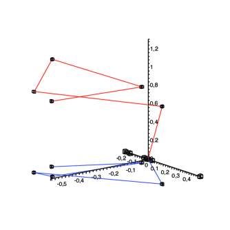
Figure III.1: an isotropic random walk in 3 dimensions and its projections

Another useful result about the q-Gaussian random walk $Z_{n}$, as defined by (III.4) with $q<1$, is given by

Theorem 4

If (i) $Z_{n}\in\mathbb{R}^{p}$ is a $q-$Gaussian random walk with $q<1$ and (ii) $\{a_{i}\}_{1\leq i\leq n}$ are independent random variables (independent of all $X_{i}$’s for $1\leq i\leq n$ in Eq. (III.4)) that follow a chi-distribution with $d$ degrees of freedom such that

$$d=p+2\frac{2-q}{1-q},$$ (III.7)

then the random walk

$$\tilde{Z}_{n}=\frac{1}{\sqrt{n}}\sum_{i=1}^{n}a_{i}X_{i},$$ (III.8)

is a Gaussian random walk with independent steps, each with covariance $\Lambda$.

Proof: The fact that each step $a_{i}X_{i}$ is a Gaussian vector is proved in 3NC . The covariance matrix of $a_{i}X_{i}$ is easily computed as

$$E(aX_{i})(aX^{t}_{i})=Ea^{2}EX_{i}X^{t}_{i}=d\frac{1}{d}\Lambda=\Lambda$$ (III.9)

and the independence of the steps results from the assumptions. $\square$

IV Conclusions

We have proved here some new results for random walks governed by distributions of the power-law type. Summing up:

• In the case $q>1$ (Section II) we saw that a stochastic representation of the point reached after $n$ steps of the walk can be expressed explicitly for all $n$.

• Moreover, Theorem 2 allows one to highlight the fact that, even in the Lévy (infinite covariance) case, the superstatistics framework remains still valid, a rather remarkable result

• In the case $q<1$ (Section III), we ascertained that the random walk can be interpreted as a projection of an isotropic random walk, i.e. a random walk with fixed length steps and uniformly distributed directions.

• Moreover, Theorem 4 shows that a $q-$Gaussian random walk with $q<1$, each step of which being subjected to independent, multiplicative chi-distributed fluctuations, is exactly a Gaussian random walk, a fact that can be qualified as a dual superstatistics.

- (1) B. Hughes, Random Walks and Random Environments, Vol. I (Oxford University Press, Oxford, 1995) and references therein. See in particular Sec. 2.1 for historical aspects.
- (2) S. Abe and Y. Okamoto, Eds. Nonextensive statistical mechanics and its applications (Springer, Berlin, 2001).
- (3) M. Gell-Mann and C. Tsallis, Eds. 2004 Nonextensive Entropy: Interdisciplinary applications (Oxford: Oxford University Press).
- (4) G. Kaniadakis, M. Lissia and A. Rapisarda, Eds., 2002 Nonextensive statistical mechanics and physical applications, Physica A (Special) 305.
- (5) Special Issue, Europhysics-news, 36 (2005); M. Buchanan, New Scientist 187, 34 (2005)
- (6) C. Anteneodo, Physica A 358, 289 (2005) .
- (7) C. Vignat, A. Plastino, and A. R. Plastino, Il Nuovo Cimento B 120, 951 (2005).
- (8) C. Vignat and A. Plastino, Phys. Lett. A 343 (2005) 411 (and references therein); Physica A 361 , 139 (2006).
- (9) C. Vignat and A. Plastino, Physica A 365, 167 (2006).
- (10) C. Beck and E. G. D. Cohen, Physica A 322, 267 (2003).
- (11) C. Beck, Continuum Mech. Thermodyn. 16, 293 (2004).
- (12) C. Beck, Phys. Rev. Lett. 87, 180601 (2001).
- (13) C. Beck and E.G.D. Cohen, Physica A 344, 393 (2004).
- (14) C. Beck, Physica A 342, 139 (2004).
- (15) C. Beck, Physica D 193, 195 (2004).
- (16) H. Touchette and C. Beck, Phys. Rev. E 71, 016131 (2005).
- (17) E. Lukacs, A characterization of the Gamma distribution, Annals of Math. Stat., 26, 319-324 (1965).
- (18) J.M. Dickey, Three multidimensional-integral identities with Bayesian applications, The Annals of Mathematical Statistics, 39-5, 1615-1627 (1968).
- (19) denotes equality in distribution.
- (20) M.Z. Bazant, Introduction to random walks and diffusion, Lectures Notes, 2001, http://www-math.mit.edu/~bazant/teach
- (21) B. V. Gnedenko and A. N. Kolmogorov, Limit distributions for sums of independent random variables, Addison-Wesley, 1968.
- (22) W. Feller, An Introduction to Probability Theory and Its Applications, Second Edition, John Wyley and Sons, 1965
- (23) C. Tsallis, Milan Journal of Mathematics, volume 73-1, 145-176 (2005).