Monte Carlo study of the antiferromagnetic three-state Potts model
with staggered polarization field on the square lattice

Abstract

Using the Wang-Landau Monte Carlo method, we study the antiferromagnetic (AF) three-state Potts model with a staggered polarization field on the square lattice. We obtain two phase transitions; one belongs to the ferromagnetic three-state Potts universality class, and the other to the Ising universality class. The phase diagram obtained is quantitatively consistent with the transfer matrix calculation. The Ising transition in the large nearest-neighbor interaction limit has been made clear by the detailed analysis of the energy density of states.

I Introduction

The $q$-state Potts model is one of the basic models for studying phase transitions Pott52 . The properties of the antiferromagnetic (AF) Potts models are more complex than those of the ferromagnetic (F) ones. The phase transitions of the AF Potts models depend heavily on the number of states $q$, the details of lattice structure, etc. The AF three-state ($q=3$) Potts model on a square lattice exhibits a second-order transition at $T$=0 with the Gaussian criticality Lena67 ; Baxt70 . While this model with only the nearest-neighbor (NN) interactions has been studied in detail Lena67 ; Baxt70 ; Nijs82 ; Burt97 ; Wang89 ; Sala98 ; Ferr99 ; Card01 , the effect of the next-nearest-neighbor (NNN) interactions has many interesting problems to explore Nijs82 ; Otsu04 . Quite recently, the present authors have studied the square-lattice AF three-state Potts model with a staggered polarization field Otsu04 . By the use of the exact diagonalization calculation of the transfer matrix and the phenomenological renormalization-group analysis, two types of phase transitions have been discussed in connection with a field theoretical argument. The crossover behavior from the AF to the F three-state Potts criticality, which was proposed by Delfino DelfNATO , has been confirmed.

The exact diagonalization calculation and the Monte Carlo simulation play a complementary role in the numerical study. The energy levels obtained by the exact diagonalization are highly accurate, but the tractable size is limited. On the other hand, although the statistical errors are unavoidable because of the sampling process, the Monte Carlo simulation can deal with larger systems. Moreover, the latter can easily study the spin configuration, the probability distribution of the order parameter, etc. Recently, several attempts have been proposed for the Monte Carlo algorithms to directly calculate the energy density of states (DOS), such as the multicanonical method berg91 ; Lee93 , and the Wang-Landau method wl .

In this paper, we study the square-lattice AF three-state Potts model with a staggered polarization field by using the Wang-Landau Monte Carlo method. We calculate the energy DOS precisely, and study the phase transitions of the model. Using the finite-size scaling (FSS), we investigate the critical properties. In Sec. II, the model and the calculation method are described. The results for phase transitions are given in Sec. III. The final section is devoted to a summary and discussions.

II Model and calculation method

We treat the AF three-state Potts model with the staggered polarization field on the square lattice $\Lambda$, whose Hamiltonian is given as

$$H=J_{1}\sum_{\langle j,k\rangle}\delta_{\sigma_{j},\sigma_{k}}-J_{2}\sum_{[j,k]}(-1)^{j}\delta_{\sigma_{j},\sigma_{k}}.$$ (1)

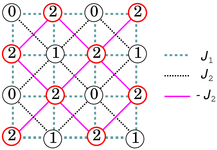
Figure 1: Schematic illustration of the AF three-state Potts model with the staggered polarized field. The sites belonging to the sublattice $\Lambda_{+}$ ($\Lambda_{-}$) are denoted by red thick (black thin) circles. The NNN interactions on the sublattice $\Lambda_{+}$ ($\Lambda_{-}$) are F (AF). An example of the ground-state configuration is also given.

Here, $\sigma_{j}=0,1,2$, and $J_{1},J_{2}>0$. The first sum is performed over the whole NN pairs $\langle j,k\rangle$, and the second sum over the whole NNN pairs $[j,k]$. Here, $(-1)^{j}=\pm 1$ for $j$ in the even (odd) sublattice $\Lambda_{\pm}$. The second term is the staggered polarization field term, which breaks the sublattice symmetry. The NN and NNN interactions are schematically shown in Fig. 1 for convenience. We also give an example of the ground-state configuration there.

In order to obtain precise numerical information we use the Wang-Landau Monte Carlo algorithm wl because of the following reasons. This type of extended ensemble methods do not suffer from the problem of the critical slowing down near the second-order phase transitions. The cluster algorithms are not so efficient for the systems with NNN couplings. We use the information of the energy DOS for the detailed study of the phase transitions. In the Wang-Landau method, a random walk in energy space is performed with a probability proportional to the reciprocal of the DOS, $1/g(E)$, which results in a flat histogram of energy distribution. Since the DOS is not known a priori, it is iteratively updated as

$$\ln g(E)\rightarrow\ln g(E)+\ln f,$$ (2)

every time a random walker visits a state with energy $E$. A large modification factor $f$ is introduced to accelerate the diffusion of the random walk in the early stage of the simulation, and it is gradually reduced to unity by checking the ‘flatness’ of the energy histogram. We set the final value of ($\ln f$) as $10^{-8}$ following the original paper by Wang and Landau wl , and then measure the energy dependence of a quantity $Q$, that is, $Q(E)$. In measuring $Q(E)$, the DOS $g(E)$ is fixed as the final one. Finally we calculate the thermal average $\langle Q\rangle_{T}$ at the temperature $T$ using the energy DOS and the Boltzmann weight as

$$\langle Q\rangle_{T}=\frac{\sum_{E}Q(E)g(E)e^{-E/T}}{\sum_{E}g(E)e^{-E/T}},$$ (3)

where the Boltzmann constant has been included in the definition of $T$.

We make simulations for several sets of $J_{2}/J_{1}$; we treat the system sizes $N=L\times L$ up to $L=64$. For the energy range of the random walk we do not cover the whole possible energy space to save computation time. The lowest energy is taken as the ground-state energy, $E=-J_{2}N$, but we set the highest energy as that takes the maximum DOS, in other words, the energy at the infinite temperature. This energy is $(2/3)J_{1}N$. We make the measurement for $4\times 10^{6}$ Monte Carlo steps per spin after the final energy DOS is obtained using the Wang-Landau process. We perform 64 independent runs for each system size in order to get better statistics and to estimate statistical errors. We estimate the statistical errors from 64 independent calculations. They could be underestimated if there are systematic errors due to the Wang-Landau method.

III Results

III.1 Specific heat

First, we present the data for the specific heat of the AF three-state Potts model with the staggered polarization field on the square lattice. We plot the temperature dependence of the specific heat for $J_{2}/J_{1}$ = 1/2, 1, and 2 in Fig. 2. The temperature is denoted in units of $T/J_{1}$ from now on unless specified else. The system sizes are $L$=16, 24, 32, 48, and 64. The statistical errors are within the width of lines.

We see two peaks in the specific heat for each $J_{2}/J_{1}$, which indicates the existence of two phase transitions clearly. The peak value for the high-temperature phase transition increases rapidly with the system size, which suggests a positive specific-heat exponent $\alpha$. The peak value for the low-temperature transition, on the contrary, increases gradually with the size. It is difficult, however, to determine whether this increase is a logarithmic divergence or a power-law one with very small $\alpha/\nu$ for these system sizes.

III.2 Order parameter

To investigate the behavior of the phase transitions in more detail, we consider the order parameters. For high-temperature phase transition, we look at the staggered magnetization for the AF Potts model, which is given by

$${M_{\rm s}}^{2}={S_{0}}^{2}+{S_{1}}^{2}+{S_{2}}^{2},$$ (4)

where

$$S_{\ell}=\frac{1}{N}\sum_{j\in\Lambda}(-1)^{j}\,\delta_{\sigma_{j},\ell},\quad\ell=0,1,2.$$ (5)

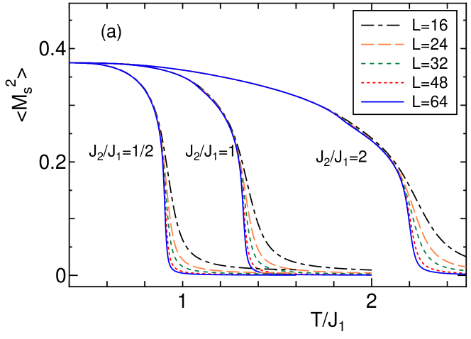
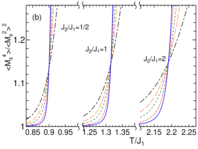
Figure 3: The high-temperature order parameter (a) and the ratio of the its moments (b) of the AF three-state Potts model with the staggered polarization field for $J_{2}/J_{1}$ = 1/2, 1, and 2. The temperature is plotted in units of $T/J_{1}$. The system sizes are $L$= 16, 24, 32, 48, and 64. The statistical errors are within the width of lines.

The order parameter $M_{\rm s}$ takes non-zero values if the ${\bf S}_{3}$ symmetry associated with the global permutations of three Potts states is broken. At the ground state of the AF three-state Potts model with the staggered polarization field, which is shown in Fig. 1, this order parameter takes the value of ${M_{\rm s}}^{2}=3/8$; we should note that the ground state is sixfold degenerate. The temperature dependence of $\langle{M_{\rm s}}^{2}\rangle$ is plotted in Fig. 3(a). The value of $J_{2}/J_{1}$ is 1/2, 1, and 2; for each $J_{2}/J_{1}$, the data for $L$=16, 24, 32, 48, and 64 are shown. We see that $M_{\rm s}$ grows below the temperature that gives a peak of the specific heat, which indicates that $M_{\rm s}$ is an appropriate order parameter for the high-temperature phase transition. The F order develops on the sublattice $\Lambda_{+}$.

For the quantitative analysis of the phase transition, we use the moment ratio, $\langle{M_{\rm s}}^{4}\rangle/\langle{M_{\rm s}}^{2}\rangle^{2}$, which is essentially the same as the Binder ratio Binder . We plot the moment ratio for the high-temperature phase transition in Fig. 3(b). Curves with different sizes cross at a single point if the corrections to FSS are negligible. The crossings of our data are very good. From the crossing point, we estimate the critical temperature. We can also estimate the critical exponent $\nu$ by the FSS analysis,

$$\langle{M_{\rm s}}^{4}\rangle/\langle{M_{\rm s}}^{2}\rangle^{2}=f(tL^{1/\nu}),$$ (6)

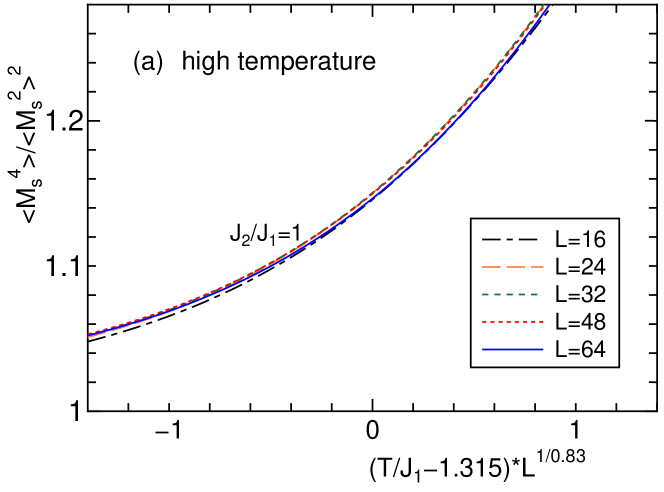
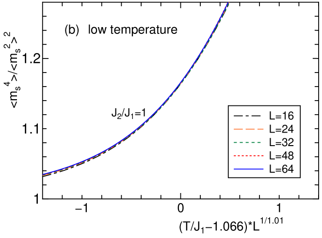
Figure 4: Scaling plot of the moment ratios of the AF three-state Potts model with the staggered polarization field for $J_{2}/J_{1}$ = 1. We plot both the high-temperature order parameter (a) and the low-temperature one (b). The temperature is plotted in units of $T/J_{1}$. The system sizes are $L$= 16, 24, 32, 48, and 64.

where $t=(T-T_{c})/T_{c}$. We show the FSS plot of the moment ratio for $J_{2}/J_{1}$=1, for example, in Fig. 4(a). We see a very good FSS. We can also estimate the critical exponent $\beta/\nu$ using the FSS relation,

$$\langle{M_{\rm s}}^{2}\rangle_{T=T_{c}}\sim L^{-2\beta/\nu}.$$ (7)

We tabulate the estimates of $T_{c}$, $\nu$, and $\beta/\nu$ for the high-temperature phase transition in Table 1. The results for $J_{2}/J_{1}$ = 1/4 and 4 are also given there. The numbers in the parentheses denote the uncertainty in the last digits. We use the least-square fitting for the FSS estimates without considering the corrections to FSS. The statistical errors are estimated from 64 independent runs. We see from Table 1 that $\nu$ is consistent with the F three-state Potts value of $\nu=5/6=0.833$. We also find that $\beta/\nu$ is compatible with the F three-state Potts value of $\beta/\nu=2/15=0.133$. The estimates of the moment ratio at $T=T_{c}$ are also given in Table 1. This value is consistent with that for the F three-state Potts model, $1.16\pm 0.01$ Tome .

Here, the corrections to FSS have not been considered explicitly for the estimate of the critical temperature and critical exponents. The $J_{2}/J_{1}$ dependences of the estimated critical exponents and the moment ratio at $T=T_{c}$ are small, but the deviations from the values for the F three-state Potts model become larger for small $J_{2}/J_{1}$. This behavior is prominent for the moment ratio at $T=T_{c}$, which is more accurate than the critical exponents. This is consistent with the fact that the system on the sublattice $\Lambda_{+}$ is nothing but the F three-state Potts model for large $J_{2}/J_{1}$ limit, which determines the renormalization-group flow Otsu04 .

Next consider the low-temperature phase transition. The ${\bf S}_{3}$ symmetry is already broken in the sublattice $\Lambda_{+}$; we should consider the symmetry breaking within the sublattice $\Lambda_{-}$. Then, we may consider the following quantity as the order parameter for the low-temperature phase transition:

$${m_{\rm s}}^{2}={s_{0}}^{2}+{s_{1}}^{2}+{s_{2}}^{2},$$ (8)

where

$$s_{\ell}=\frac{1}{N}\sum_{k\in\Lambda_{-}}(-1)^{k}\,\delta_{\sigma_{k},\ell},\quad\ell=0,1,2.$$ (9)

We only look at the spins on the sublattice $\Lambda_{-}$. The sublattice $\Lambda_{-}$ forms a $\sqrt{2}\times\sqrt{2}$ square lattice, and we divide the sublattice $\Lambda_{-}$ into two further sublattices. For these further sublattices, we take $(-1)^{k}=\pm 1$ depending on the values of $k$, even or odd. This order parameter essentially represents the AF Ising order in the sublattice $\Lambda_{-}$. At the ground state the low-temperature order parameter, Eq. (8), takes the value of ${m_{\rm s}}^{2}=1/8$.

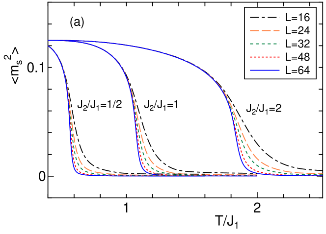
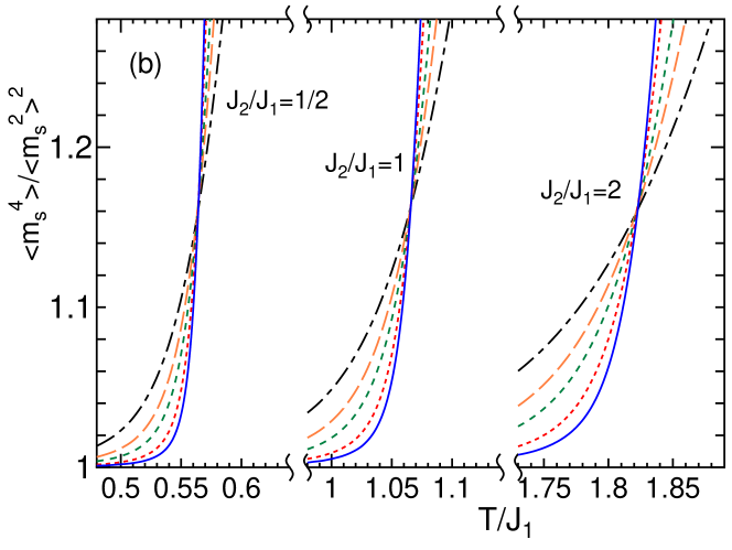
Figure 5: The low-temperature order parameter (a) and the ratio of the its moments (b) of the AF three-state Potts model with the staggered polarization field for $J_{2}/J_{1}$ = 1/2, 1, and 2. The temperature is plotted in units of $T/J_{1}$. The system sizes are $L$= 16, 24, 32, 48, and 64. The statistical errors are within the width of lines.

In Fig. 5(a) we plot the order parameter of the low-temperature phase transition, Eq. (8). This time, $m_{\rm s}$ grows below the temperature that gives a lower peak of the specific heat; we see that $m_{\rm s}$ is an appropriate order parameter for the low-temperature phase transition. We can consider the moment ratio associated with the low-temperature order parameter; $M_{\rm s}$ will be replaced by $m_{\rm s}$ in Eq. (6). This moment ratio is plotted in Fig. 5(b). Again, we see the crossing of the curves with different sizes. Using the FSS analysis, we estimate $T_{c}$, $\nu$, and $\beta/\nu$, and they are tabulated in Table 1. The FSS plot of the moment ratio for $J_{2}/J_{1}$=1 is given in Fig. 4(b), for example. The estimated exponents shown in Table 1 suggest that the exponents $\nu$ and $\beta/\nu$ are consistent with the two-dimensional (2D) Ising values, 1 and 1/8=0.125, respectively. The moment ratio at $T=T_{c}$ is also given in Table 1. The Ising value for the finite system with aspect ratio 1:1 is rigorously calculated as 1.1679229(47) Francesco . The coincidence with this value is very good.

The $J_{2}/J_{1}$ dependences of the estimated critical exponents and the moment ratio at $T=T_{c}$ are very small, but the deviations from the Ising values become slightly larger for large $J_{2}/J_{1}$, which is the opposite direction from the case of the high-temperature transition.

III.3 Phase diagram

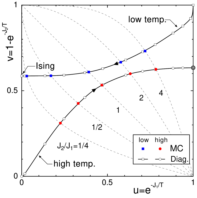
Figure 6: Phase diagram of the AF three-state Potts model with the staggered polarization field. The filled circle (red) and filled square (blue) represent the estimate of high-temperature and low-temperature $T_{c}$’s in the present Monte Carlo study, whereas the open marks represent those by the transfer-matrix calculation Otsu04 . The F three-state Potts point $(u,v)=(1,(3-\sqrt{3})/2=0.6340)$ is shown by the double circle, and a point with 2D-Ising criticality on the $v$-axis is shown by the arrow.

From the list of the estimates of the two critical temperatures given in Table 1 for $J_{2}/J_{1}$ = 1/4, 1/2, 1, 2, and 4, we discuss the phase diagram. In Fig. 6 we plot the phase diagram in the parameter space of $(u,v)=(e^{-J_{1}/T},1-e^{-J_{2}/T})$, which is the same as the previous transfer-matrix study Otsu04 . The trajectories of $J_{2}/J_{1}$=1/4, 1/2, 1, 2, and 4 are shown by dotted curves starting from $T=0$ [$(u,v)=(0,1)$] to $T=\infty$ [$(u,v)=(1,0)$]. The filled circle (red) and filled square (blue) represent the estimate of high-temperature and low-temperature $T_{c}$’s in the present study, respectively, and they are compared with the previous estimates by the transfer-matrix calculation Otsu04 , which are given by open marks. These two results are consistent with each other, which shows the reliability of both calculations. In the transfer-matrix calculation Otsu04 , the characterization of the excitation levels was important. In the present MC simulation, we have employed the method to calculate the DOS accurately, and have made the appropriate choice of the order parameters. With these careful treatments, we have obtained the accurate enough phase diagram.

From the behavior of the corrections, we can see the renormalization-group flow of the phase boundary, which is consistent with Zamolodchikov’s $c$-theorem Zamo86 . For the high-temperature phase transition, the flow starts from the Gaussian point $(u,v)=(0,0)$ to the F three-state Potts point $(u,v)=(1,(3-\sqrt{3})/2=0.6340)$, which is shown by the double circle. On the other hand, for the low-temperature phase transition, the flow starts another Gaussian point $(u,v)=(1,1)$ to a point with 2D-Ising criticality on the $v$-axis, which is shown by the arrow in Fig. 6.

This Ising transition in the large $J_{1}$ limit (on the $v$-axis) is a subtle problem. In Ref. Otsu04 , the inverse critical temperature was estimated as $J_{2}/T_{c}$ = 0.8820, which is slightly larger than the Ising value of $\ln(\sqrt{2}+1)$=0.8814 [$v=1-e^{-J_{2}/T}$=$2-\sqrt{2}$=0.5858].

III.4 Large NN interaction limit

Here we examine the Ising transition in the large $J_{1}$ limit. If we consider only the NN interaction term in Eq. (1), the energies of the ground states and the first excited states are 0 and $J_{1}$, respectively. The NNN interaction term takes the energy between $-J_{2}N$ to $J_{2}N$. Thus, for the case of $J_{2}/J_{1}\leq 1/(2N)$, we have to consider only the ground-state configuration for NN interactions. We make a Wang-Landau type MC simulation for our model with this restriction. That is, only the ground-state configurations for the NN AF three-state Potts model are allowed, and we calculate the energy DOS for the NNN interactions.

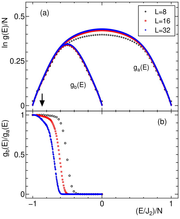
Figure 7: (a) The energy DOS of the AF three-state Potts model with the staggered polarization field in the subspace of the ground states of the NN AF three-state Potts model, $g_{a}(E)$, and that of the pure Ising model, $g_{b}(E)$. The critical energy of the Ising transition point, $(E/J_{2})/N$ = $-(2+\sqrt{2})/4=-0.8536$, is shown by an arrow. (b) The ratio of two DOS’s, $g_{b}(E)/g_{a}(E)$.

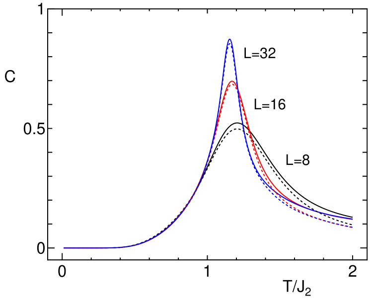
Figure 8: Comparison of the specific heat between that for the present model in the subspace of the ground states of the NN AF three-state Potts model (solid line) and that for the pure Ising model (dotted line).

In Fig. 7(a), we plot the DOS for this restricted model in the subspace of the ground states of the NN AF three-state Potts model, $g_{a}(E)$. If all the spins on the sublattice $\Lambda_{+}$ take one of the three states (the complete F three-state Potts order) and the spins on the sublattice $\Lambda_{-}$ take either one of the other two states, these spin configurations are parts of the ground states of the NN AF three-state Potts model, and are called the broken-sublattice-symmetry states in the study of the AF Potts models Banavar . Then, the spins on the $\sqrt{2}\times\sqrt{2}$ sublattice $\Lambda_{-}$ are regarded as the AF Ising model with the NN interactions. The energy DOS of this pure Ising model, $g_{b}(E)$, is also shown in Fig. 7(a). The extra three-times degeneracy due to three complete F states in the sublattice $\Lambda_{+}$ was taken into account. The phase transition is determined by the structure of the energy DOS near the Ising critical energy, $(E/J_{2})/N$ = $-(2+\sqrt{2})/4=-0.8536$, which is shown by an arrow in Fig. 7. In this region two DOS’s look close when the logarithmic scale is used. However, we understand the very small difference in the critical temperature from the structure of DOS. We plot the ratio of $g_{b}(E)/g_{a}(E)$ in Fig. 7(b). Then, we find that this ratio becomes smaller for larger system size $L$. This means that we cannot ignore contributions from the spin configurations which are not the pure Ising one. Therefore, we may conclude that although this transition belongs to the Ising universality class, the critical temperature, which is not a universal quantity, is slightly modified from that of the pure Ising model. Since the number of configurations are larger than that for the pure Ising model, the critical temperature $T_{c}/J_{2}$ becomes slightly lower than that for the pure Ising model. In Fig. 8, we compare the specific heat calculated from two DOS’s, which give almost the same behavior but there is still a small difference.

In the MC method to calculate DOS we obtain the relative ratio of DOS’s at different energies $E_{1}$ and $E_{2}$, $g(E_{1})/g(E_{2})$. The absolute value of $g(E)$ can be obtained with other conditions. For the Ising model, as an example, the equation to give the total number of states, $\sum_{E}g(E)=2^{N}$, is such a condition. There is also a boundary condition if the ground-state degeneracy is known. The ground state of the present model is sixfold degenerate; thus $g(E=-J_{2}N)$=6. Then, with this condition we can calculate the total number of states, $\sum_{E}g(E)$. This value is nothing but the ground-state degeneracy for the NN AF three-state Potts model, because we restrict ourselves to the subspace of the ground states of the AF three-state Potts model. To confirm the reliability of our calculation, we calculate the normalized ground-state entropy of the AF three-state Potts model, $S/N=[\ln\sum_{E}g(E)]/N$, as a function of $L$ with this procedure, $S(1)/N$, and they are tabulated in Table 2. More direct way of obtaining the ground-state entropy is to calculate the ground-state DOS of the three-state Potts model with the condition of $\sum_{E}g(E)=3^{N}$. This procedure was employed in the study of the three-dimensional AF Potts models Yama01 . The result of this direct way, $S(2)/N$, is also tabulated in Table 2. These two results coincide with each other completely. This indicates the effectiveness of the treatment of this subsection, that is, we have applied the Wang-Landau method to the present model with the restricted configurations. The normalized ground-state entropy for the AF three-state Potts model on the square lattice is exactly known as $\ln(4/3)^{3}/2=0.431523$ for the infinite size limit ent . The extrapolation of the data of $S/N$ shown in Table 2 as a polynomial of $1/N$ yields $0.43154+1.10\times(1/N)$, which is consistent with the exact value within the statistical errors. We should mention that the ground-state entropy of the AF Potts model was extensively studied numerically by Shrock and Tsai Shrock .

IV Summary and discussions

We have studied the square-lattice AF three-state Potts model with a staggered polarization field using the Wang-Landau MC method. We have obtained two phase transitions, which belong to the ferromagnetic three-state Potts and Ising universality classes. We have confirmed the quantitative consistency of the phase diagram with the transfer-matrix study Otsu04 . This consistency shows the reliability of both calculations, the previous transfer-matrix calculation and the present MC study. A special attention has been paid to the Ising transition in the large $J_{1}$ limit. The origin of the slight difference of the transition point from the value of the pure Ising model has been made clear by the detailed analysis of the energy DOS. As a check of the method, we have calculated the ground-state residual entropy for the AF three-state Potts model by two ways.

The specific heat has singularities at the critical points as shown in Fig. 2. The specific-heat amplitudes have information on the crossover behavior Cardy . We can study the Gaussian to F three-state Potts and the Gaussian to Ising crossovers by the $J_{2}/J_{1}$ dependence of the specific-heat amplitudes. The detailed study on this crossover will be left to a separate study.

We here make comments on the Wang-Landau method. In calculating the thermal average of $M_{\rm s}$ and $m_{\rm s}$, we have used the microcanonical average $M_{\rm s}(E)$ and $m_{\rm s}(E)$ as in Eq. (3). If the energy DOS g(E) is not converged enough, it may cause a systematic error in calculating the thermal average. The use of the joint DOS $g(E,Q)$ may help the convergence. We have checked for smaller system sizes that the present calculations with the microcanonical average and those using the joint DOS give the same results within the statistical errors. The second comment is as follows. We may employ a random walk in the space of two parameters, $\sum_{\langle j,k\rangle}\delta_{\sigma_{j},\sigma_{k}}$ and $\sum_{[j,k]}(-1)^{j}\delta_{\sigma_{j},\sigma_{k}}$, instead of the single parameter of the total energy $E$. Then, we can get all the information for different $J_{2}/J_{1}$ from the result of a single simulation. Actually, for smaller system sizes ($L\leq 16$), the two-parameter random walk method works well. However, simulations with fixed $J_{1}$ and $J_{2}$ are more effective for larger sizes.

In this paper, we have considered the staggered polarization field for the NNN interaction. The effect of the F NNN interaction is also interesting. In this case, the system has the same universality class as the six-state clock model, which yields two Berezinskii-Kosterlitz-Thouless transitions Bere71 ; Kost73 . The precise calculation of this problem has been quite recently performed by using the level-spectroscopy method Nomu95 based on the exact diagonalization of the transfer matrix Otsu05 . A complementary study of the AF Potts model with the F NNN interaction using the Monte Carlo method is highly needed, and this research is now in progress.

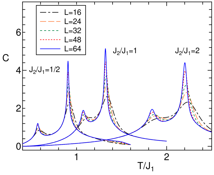
Figure 2: The specific heat of the AF three-state Potts model with the staggered polarization field for $J_{2}/J_{1}$ = 1/2, 1, and 2. The temperature is plotted in units of $T/J_{1}$. The system sizes are $L$= 16, 24, 32, 48, and 64. The statistical errors are within the width of lines.

Table 1: The list of $T_{c}$, $\nu$, $\beta/\nu$, and moment ratio at $T=T_{c}$ for two phase transitions. The temperature is represented in units of $T/J_{1}$.

$J_{2}/J_{1}$	$T_{c}$	$\nu$	$\beta/\nu$	ratio
high temp.
1/4	0.6720(2)	0.83(1)	0.105(4)	1.120(6)
1/2	0.9000(3)	0.83(1)	0.114(4)	1.138(6)
1	1.3150(5)	0.83(1)	0.122(4)	1.148(6)
2	2.1911(5)	0.83(1)	0.126(4)	1.154(6)
4	4.0840(5)	0.82(1)	0.127(4)	1.154(6)
low temp.
1/4	0.2830(2)	1.00(1)	0.120(4)	1.162(4)
1/2	0.5642(3)	1.01(1)	0.123(4)	1.165(4)
1	1.0657(5)	1.01(1)	0.123(4)	1.164(4)
2	1.8228(5)	0.99(1)	0.125(4)	1.164(4)
4	3.0240(5)	0.98(1)	0.123(4)	1.155(4)

Table 2: The estimate of the residual entropy per spin of the AF three-state Potts model on the square lattice. Two procedures are employed to calculate $S/N$. (1) The total number of states for the subspace of the ground states of the AF three-state Potts model is calculated. (2) The direct way to calculate the ground-state DOS of the three-state Potts model is used with the condition of $\sum_{E}g(E)=3^{N}$.

$L$	$S(1)/N$	$S(2)/N$
16	0.43569(8)	0.43575(11)
24	0.43345(6)	0.43353(7)
32	0.43259(4)	0.43262(9)
48	0.43198(3)	0.43202(15)
64	0.43176(5)	0.43185(10)

References

-
(1)
Potts R B 1952 Proc. Cambridge. Philos. Soc. 48 106
Wu F Y 1982 Rev. Mod. Phys. 54 235 -
(2)
Lieb E H 1967 Phys. Rev. 162 162
Lieb E H 1967 Phys. Rev. Lett. 18 692 -
(3)
Baxter R J 1970 J. Math. Phys. (N.Y.) 11 3116
Baxter R J 1982 Proc. Roy. Soc. London A383 43 - (4) den Nijs M P M, Nightingale M P and Schick M 1982 Phys. Rev. B 26 2490
- (5) Burton Jr. J K and Henley C L 1997 J. Phys. A: Math. Gen. 30 8385
- (6) Wang J S, Swendsen R H and Kotecký R 1989 Phys. Rev. Lett. 63 109
- (7) Salas J and Sokal A D 1998 J. Stat. Phys. 92 729
- (8) Ferreira S J and Sokal A D 1999 J. Stat. Phys. 96 461
- (9) Cardy J, Jacobsen J L and Sokal A D 2001 J. Stat. Phys. 105 25
- (10) Otsuka H and Okabe Y 2004 Phys. Rev. Lett. 93 120601
- (11) Delfino G, in Proceedings of the NATO advanced research workshop on Statistical field theories, edited by Cappelli A et al. (Kluwer A.P., 2002); eprint hep-th/0110181
-
(12)
Berg B A and Neuhaus T 1991 Phys. Lett. B 267 249
Berg B A and Neuhaus T 1992 Phys. Rev. Lett. 68 9 - (13) Lee J 1993 Phys. Rev. Lett. 71 211
-
(14)
Wang F and Landau D P 2001 Phys. Rev. Lett. 86 2050
Wang F and Landau D P 2001 Phys. Rev. E 64 056101 - (15) Binder K 1981 Z. Phys. B 43 119
- (16) Tomé T and Petri A 2002 J. Phys. A: Math. Gen. 35 5379
-
(17)
Di Francesco P, Saleur H and Suber J B 1987
Nucl. Phys. B 290 [FS20] 527
Di Francesco P, Saleur H and Suber J B 1988 Europhys. Lett. 5 95 - (18) Zamolodchikov A B 1986 Zh. Eksp. Teor. Fiz. 43 565 [1986 JETP Lett. 43 730]
-
(19)
Banavar J B, Grest G S and Jasnow D
1980 Phys. Rev. Lett. 45 1424
Banavar J B, Grest G S and Jasnow D 1982 Phys. Rev. B 52 4639 - (20) Yamaguchi C and Okabe Y 2001 J. Phys. A: Math. Gen. 34 8781
- (21) Park H and Widom M 1989 Phys. Rev. Lett. 63 1193
-
(22)
Shrock R and Tsai S H 1997 J. Phys. A: Math. Gen. 30 495
Shrock R and Tsai S H 1998 Phys. Rev. E 58 4332 - (23) Cardy J L 1996 Scaling and Renormalization in Statistical Physics (Cambridge University Press, Cambridge)
- (24) Berezinskii V L 1971 Zh. Eksp. Teor. Fiz. 61 1144 [1972 Sov. Phys. JETP 34 610]
-
(25)
Kosterlitz J M and Thouless D J 1973
J. Phys. C: Solid State Phys. 6 1181
Kosterlitz J M 1974 J. Phys. A: Math. Gen. 7 1046 - (26) Nomura K 1995 J. Phys. C: Solid State Phys. 28 5451
- (27) Otsuka H, Mori K, Okabe Y and Nomura K 2005 Phys. Rev. E 72 046103