Understanding the Frequency Distribution of Mechanically Stable Disk Packings

Abstract

Relative frequencies of mechanically stable (MS) packings of frictionless bidisperse disks are studied numerically in small systems. The packings are created by successively compressing or decompressing a system of soft purely repulsive disks, followed by energy minimization, until only infinitesimal particle overlaps remain. For systems of up to $14$ particles most of the MS packings were generated. We find that the packings are not equally probable as has been assumed in recent thermodynamic descriptions of granular systems. Instead, the frequency distribution, averaged over each packing-fraction interval $\Delta\phi$, grows exponentially with increasing $\phi$. Moreover, within each packing-fraction interval MS packings occur with frequencies ${f}_{k}$ that differ by many orders of magnitude. Also, key features of the frequency distribution do not change when we significantly alter the packing-generation algorithm—for example frequent packings remain frequent and rare ones remain rare.

These results indicate that the frequency distribution of MS packings is strongly influenced by geometrical properties of the multidimensional configuration space. By adding thermal fluctuations to a set of the MS packings, we were able to examine a number of local features of configuration space near each packing. We measured the time required for a given packing to break to a distinct one, which enabled us to estimate the energy barriers that separate one packing from another. We found a gross positive correlation between the packing frequencies and the heights of the lowest energy barriers $\epsilon_{0}$; however, there is significant scatter in the data. We also examined displacement fluctuations away from the MS packings to assess the size and shape of the local basins near each packing. The displacement modes scale as $d_{i}\sim\epsilon_{0}^{\gamma_{i}}$ with $\gamma_{i}$ ranging from approximately $0.6$ for the largest eigenvalues to $1.0$ for the smallest ones. These scalings suggest that the packing frequencies are not determined by the local volume of configuration space near each packing, which would require that the dependence of $f_{k}$ on $\epsilon_{0}$ is much stronger than the dependence we observe. The scatter in our data implies that in addition to $\epsilon_{0}$ there are also other, as yet undetermined variables that influence the packing probabilities.

I Introduction

Despite intense study over the past several decades, glassy and amorphous materials are still poorly understood. For example, a fundamental explanation for the stupendous rise in the viscosity of fragile glass-forming liquids as the temperature is lowered near the glass transition is still lacking debenedetti . Also, the response of glassy and amorphous systems to applied stress is difficult to predict because these systems display complex spatio-temporal dynamics, such as shear bands fu ; varnik , strongly non-affine and cooperative motion maloney ; tanguy , and dynamical heterogeneities ediger . Even basic questions concerning the nature of stress and structural relaxation have not been adequately addressed. Important open questions include 1) what are the characteristic rearrangement events that lead to stress and structural relaxation, 2) how many particles are involved in such rearrangement events, and 3) are these events correlated and over what length and time scales?

An extremely useful concept for understanding the dynamical and mechanical properties of glassy systems has been the potential energy landscape (PEL) formalism stillinger . The PEL is the highly multi-dimensional potential energy function that depends on all of the configurational degrees of freedom of the system. It has been shown that the equation of state shell ; nave and dynamical quantities keyes ; heuer such as the diffusion constant and viscosity of supercooled liquids and glasses can be calculated in terms of geometrical features of the PEL like local potential energy minima and low-order saddle points. Related studies have also been performed on hard spheres to understand the glass transition in these model systems. A significant focus of this research has been to explain kinetic arrest in terms of decreasing free volume salsburg ; sastry2 and configurational entropy speedy_chem_phys ; speedy_biophys_chem near the glass transition.

In this article we investigate particle packings and features of the potential energy landscape in 2d bidisperse systems of frictionless disks. The disks interact via a finite-range continuous repulsive potential. We focus on mechanically stable (MS) packings with vanishing particle overlaps. In these mechanically stable packings any particle displacement results in an increase of the potential energy, i.e., leads to overlap between particles. Thus the set of MS packings in our system is equivalent to the set of collectively jammed states torquato for hard disks. However, since we consider particles that interact via a continuous potential, we can explore not only geometrical features of configuration space in the neighborhood of a given collectively jammed state, but also properties of the energy landscape near a given mechanically stable packing.

An important feature of the present work (and our related earlier study xu ) is that we focus on small systems containing $14$ or fewer particles. Related studies of small hard disk systems have been carried out previously bs ; bsv , but these did not address questions concerning the frequency with which MS packings occur, which is the main focus of this work. We confine our studies to small systems for several reasons. First, we believe that understanding properties of small nearly jammed systems is crucial to developing a theoretical explanation for slow stress and structural relaxation in large glassy and amorphous systems. Second, in small systems we are able to generate nearly all of the mechanically stable disk packings, which enables us to accurately measure the frequency with which different MS packings occur. Also, detailed results obtained for small systems of different size can be extrapolated and used to infer properties of glassy materials in the large-system limit.

Results from a number of recent studies emphasize that small subsystems are important for understanding the slow dynamics displayed in supercooled liquids and glasses. For example, experiments on colloidal glasses weeks1 ; weeks2 show that slow relaxation in glassy materials occurs through local cage breaking events. Caging behavior has also been shown in a number of computer simulations of hard and soft particles, for example in Refs. doliwa ; thirumalai ; miyagawa .

Another indication that small subsystems play an important role in determining the dynamics of glass-forming liquids can be found in the results of recent numerical simulations of large binary hard-disk systems in Ref. donev . Using an appropriately defined signature of the kinetic glass transition, these authors have shown that a slowly quenched system falls out of equilibrium at packing fractions $\phi$ in the range $0.77\lesssim\phi\lesssim 0.8$ (the larger packing fractions correspond to slower quench rates). As revealed by our recent study xu (see also the results presented herein), this is the packing-fraction range where the maximum of the density of MS packings occurs for small systems of $N\gtrsim 12$ particles. We believe that this is not a coincidence.

The important role of small subsystems in dense hard-particle fluids stems from the fact that small systems become geometrically jammed (i.e., the system cannot rearrange) at packing fractions where significant free volume is still available for the motion of particles in their local cages. In contrast, for macroscopic systems even infinitesimal free volume per particle makes structural rearrangements geometrically possible.

Such observations suggest that one should seek macroscopic descriptions of glass-forming materials in terms of many coupled, nearly jammed small subdomains. At a packing fraction at which small subdomains become geometrically jammed, rearrangements can occur only if a domain is sufficiently uncompressed. Large local density fluctuations, however, occur infrequently, because of the low compressibility of the surrounding domains at packing fractions above the dynamic glass transition. Hence, the structural relaxation time is extremely large. A picture similar to the one put forward by Adam and Gibbs over $40$ years ago adam can also be constructed for systems of particles interacting via continuous potentials. In this case, relevant packing fractions can be defined using a temperature-dependent effective particle diameter.

A small subsystem of a macroscopic system corresponds to a subspace in configuration space. Thus, an approach that describes the dynamics of glass-forming liquids in terms of a set of small coupled subsystems should help to reconcile the local picture of glassy materials (e.g., trap models bouchaud ) with the global PEL view. However, before predictive theories can be constructed based on the ideas outlined above, one needs to obtain a more complete understanding of the behavior of small nearly jammed systems.

An analysis of MS packings in small systems is relevant not only for understanding the slow dynamics of glass-forming liquids, but also for explaining the meaning of random-close packing in macroscopic athermal amorphous materials. We now turn to this aspect of the problem.

In MS packings composed of touching (but not overlapping) disks, the number of degrees of freedom is less than or equal to the number of constraints. Thus, MS packings, or collectively jammed states, can be represented by single points in configuration space. In small systems we are able to generate nearly all mechanically stable disk packings. Thus, we can investigate, separately, the number of distinct packings that exist in a given interval of packing fraction $\phi$ (i.e., the density of MS packings) and the probability with which these packings occur for a given generation protocol xu .

An analysis of the protocol-independent density of MS packings and protocol-dependent probabilities for each distinct packing allows us to address the question of why random close packing seems to be a well defined quantity (i.e., many distinct generation protocols give similar values for it, for example in Refs. ohern_short ; ohern_long ; silbert ; makse ), but it is also a poorly defined concept because other protocols, for example, those that allow slow thermal quench rates, yield a continuous range of packing fractions at which jammed states occur torquato2 .

In our opinion, questions concerning random close packing have not yet been fully resolved. In particular, although the maximally random jammed (MRJ) state as described in Ref. torquato2 is a useful and important concept, we believe that it is not the final answer. For example, MRJ involves an arbitrary choice of how to characterize order in the system and does not address the question of why a wide class of generation protocols yield similar values for random-close packing.

In our recent paper xu we argued that the random close packing density corresponds to the position of the peak in the density of MS packings $\rho(\phi)$, which becomes a $\delta$-function in the infinite system-size limit. As opposed to the protocol-dependent probability density $P(\phi)$ for obtaining a packing at a given $\phi$, the density of MS packings is a protocol-independent quantity. Unless a given protocol is strongly biased toward states in the tail of the distribution $\rho(\phi)$, for example those protocols that involve significant thermalization, a well-defined random close packed density is obtained in the large system limit. This explains why many quite distinct protocols consistently yield similar values for the random close packed density $\phi_{\rm rcp}$.

This explanation, while quite plausible, leaves a number of important issues unresolved. For example, we find that individual MS packings occur with extremely different frequencies even for a typical fast-quench protocol xu . Two MS packings at approximately the same packing fraction $\phi$ but with drastically different frequencies are shown in Fig. 1. There are no striking structural differences between these two MS packings, yet, the packing shown in Fig. 1(a) is $10^{6}$ times less frequent than that in Fig. 1(b). Moreover, we find that there are many more infrequent MS packings than frequent ones.

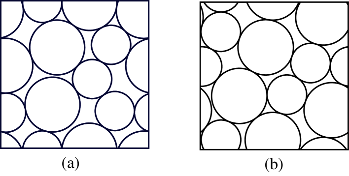
Figure 1: Snapshot of (a) a rare mechanically stable packing at $\phi\approx 0.82$ and (b) another MS packing $\phi\approx 0.83$ that is $10^{6}$ times more frequent.

An important issue is what determines whether a particular MS packing is frequent or rare. Although it is clear that the particular protocol chosen to generate the MS packings plays a role in determining the frequency distribution torquato2 , we argue that geometrical features of the PEL also strongly influence the frequency distribution. First, our protocols, which involve a sequence of compression and decompression steps followed by energy minimization do not target any particular MS packings. Yet, the probabilities of different MS packings vary by many orders of magnitude. Moreover, as we will show below, even when we significantly alter the protocol used to generate the MS packings, the most frequent packings remain frequent and the rare packings remain rare.

The question of what gives rise to the extremely diverse probabilities of different MS packings is not only important for the analysis of random close packing, but also for developing statistical descriptions of granular materials and other athermal systems. For example, it has been assumed in Edwards’ entropy descriptions of granular media mehta ; makse2 that different jammed packings occur with approximately equal weights. Similar assumptions are also usually employed in PEL theories of glassy materials debenedetti2 . However, these assumptions should be reexamined, since analogous geometric features are likely to control the frequency distributions of relevant states in these systems as in our studies of the frequency of MS packings. Understanding the reason for the enormous probability differences and the comparative roles of the frequent and infrequent states are thus important unresolved problems.

This paper is organized as follows. In Sec. II, we describe the model and protocol we use to generate the MS packings and how we classify and count each distinct packing. In Sec. III, we review our results for the density of MS packings and their frequency distribution in small 2d bidisperse systems. In Sec. IV, we investigate the correlation between local geometric features of configuration space near each MS packing and the MS packing frequencies by adding thermal fluctuations to the packings. We look for structural properties that distinguish between frequent and rare MS packings in Sec. V. In Sec. VI we introduce a simple phenomenological model to explain the dramatic variation in MS packing frequencies. We conclude and briefly discuss future research directions in Sec. VII.

II Generation and classification of mechanically stable disk packings

II.1 Model

We study the mechanical and statistical properties of MS packings in two-dimensional bidisperse systems of $N$ frictionless disks interacting via the finite-range, pairwise additive, purely repulsive spring potential of the form

$$V(r_{ij})=\frac{\epsilon}{2}(1-r_{ij}/\sigma_{ij})^{2}\Theta(\sigma_{ij}/r_{ij}-1).$$ (1)

Here $\epsilon$ is the characteristic energy scale, $r_{ij}$ is the separation between particles $i$ and $j$, $\sigma_{ij}=\left(\sigma_{i}+\sigma_{j}\right)/2$ is their average diameter, and $\Theta(x)$ is the Heaviside step function. The particles are in a square unit cell with periodic boundary conditions. The mass $m$ of all particles is assumed to be equal.

We consider $50$-$50$ binary mixtures of large and small particles with diameter ratio $1.4$. We study bidisperse mixtures because the presence of particles with different sizes inhibits crystallization (provided that the size ratio is incommensurate with a binary crystal structure). In contrast, monodisperse disk packings crystallize readily berryman ; connelly , so these systems have entirely different properties than glass-forming liquids that are the subject of our investigations. Bidisperse mixtures of disks with diameter ratio $1.4$ have been used in several previous studies speedy ; ohern_short ; ohern_long ; xu ; donev . Such mixtures thus constitute a convenient reference system for investigations of fundamental properties of amorphous and glassy materials.

In systems with finite-range purely repulsive interparticle potentials there are two general classes of potential energy minima. First, the system can possess a connected network of particle overlaps that spans the system; the sum of forces on each particle in such networks is zero. These configurations have positive total potential energy, and each displacement of the particles in the network results in an energy increase. For the second type there are no particle overlaps, all forces are zero, the total potential energy vanishes, and the particles can be moved without creating an overlap.

Our focus here is on states that are on the border between these two general classes: we assume that the system is at an energy minimum with infinitesimal particle overlaps (thus, the total energy is also infinitesimal). Since these states are assumed to be in stable mechanical equilibrium and possess vanishingly small overlaps, we term these states MS packings.

If all particles of a MS packing participate in the system spanning force network, no particle displacement is possible without creating an overlap. Occasionally, a small number of particles in a MS packing (no more than three for the small systems considered herein) do not participate in the force network. States with such free particles (rattlers) have to be treated with care in the packing generation procedures. However, we do not find that the properties of MS packings with rattlers deviate significantly from those of MS packings without rattlers.

II.2 Packing generation protocols

II.2.1 Simulation algorithms

We use here a class of packing-generation protocols that involve successive compression or decompression steps followed by energy minimization makse ; xu . The system is decompressed (or, equivalently, the particle diameters are decreased) when the energy of the system at a local minimum is nonzero; otherwise, the system is compressed. The increment by which the particle packing fraction is changed at each compression or decompression step is gradually decreased. After a sufficiently large number of steps, a MS packing with infinitesimal overlaps is thus obtained.

For each independent trial, we begin the process by choosing random initial positions for the particles at packing fraction $\phi_{0}=0.60$ (which is well below the minimum packing fraction at which MS packings occur in 2d). We then allow the system to relax, and perform a sequence of compression/decompression and relaxation steps. We can repeat this process for many independent initial conditions, generate a large number of MS packings, and measure their respective probabilities for a given protocol.

In the present study, we use two energy-minimization methods: (a) conjugate-gradient (CG) minimization algorithm or (b) molecular dynamics (MD) with dissipation proportional to local velocity differences. The conjugate-gradient method is a numerical scheme that begins at a given point in configuration space and moves the system to the nearest local potential energy minimum without traversing any energy barriers numrec . In contrast, molecular dynamics with finite damping is not guaranteed to find the nearest local potential energy minimum since kinetic energy is removed from the system at a finite rate. The system can thus surmount a sufficiently low energy barrier. In the molecular dynamics method, each particle $i$ obeys Newton’s equations of motion

$$m{\vec{a}}_{i}=\sum_{j\not=i}\Theta(\sigma_{ij}/r_{ij}-1)\left[\frac{\epsilon}{\sigma_{ij}}\left(1-\frac{r_{ij}}{\sigma_{ij}}\right)-b\vec{v}_{ij}\cdot{\hat{r}}_{ij}\right]{\hat{r}}_{ij},$$ (2)

where $\vec{a}_{i}$ is the acceleration of particle $i$, $\vec{v}_{ij}$ is the relative velocity of particles $i$ and $j$, ${\hat{r}}_{ij}$ is the unit vector connecting the centers of these particles, and $b$ is the damping coefficient. In the present study, we chose the dimensionless damping coefficient $\bar{b}=\sigma b/\sqrt{m\epsilon}=0.5$, but this will be varied in subsequent studies. In the infinite-dissipation limit $b\to\infty$ the potential energy cannot increase during a molecular-dynamics relaxation, and thus the molecular-dynamics and conjugate-gradient methods should give very similar results. We note, however, that even in this limit the two methods are not equivalent because there may be more than one energy minimum accessible from a given point in configuration space without traversing an energy barrier. In our previous studies ohern_short ; ohern_long ; xu , we used only the conjugate-gradient minimization algorithm.

II.2.2 Implementation details

In specific implementations of our MS-packing generation protocols, one needs to use appropriate numerical criteria for stopping the energy minimization process either in a configuration with overlapping particles forming a force network or in a state with no particle overlaps. For the the conjugate gradient method, we terminate the minimization process when either of the following two conditions on the potential energy per particle $V$ is satisfied: (a) two successive conjugate gradient steps $n$ and $n+1$ yield nearly the same energy value, $(V_{n+1}-V_{n})/V_{n}<\delta=10^{-16}$; or (b) the potential energy per particle at the current step is extremely small, $V_{n}<V_{\rm min}=10^{-16}$ (where $V$ is normalized by the energy-scale parameter $\epsilon$). Since the potential energy oscillates in time in the molecular dynamics method, condition (a) is replaced by the requirement that the relative potential-energy fluctuations satisfy the inequality $\langle(V-\langle V\rangle)^{2}\rangle^{1/2}/\langle V\rangle<\delta$.

Following the energy minimization, we determine whether the system should be compressed or expanded. If, $V\leq V_{\rm min}$, the system is below the jamming threshold, and thus it is compressed by $\Delta\phi$. If, on the other hand, $V>V_{\rm max}=2V_{\rm min}$, the system is decompressed by $\Delta\phi$. For the first compression or decompression step we use the packing-fraction increment $\Delta\phi=10^{-4}$. Each time the procedure switches from expansion to contraction or vice versa, $\Delta\phi$ is reduced by a factor of $2$.

For the molecular-dynamics procedure to be efficient, rattler particles with no contacts must be treated with care. When the system is near the jamming threshold, we set the velocities of rattlers to zero; we also shift the center-of-mass velocity of the remaining non-rattler particles to zero to assure momentum conservation. This modification of the energy-minimization procedure allows our stopping criteria to be implemented without change even when rattlers are present. Otherwise, the kinetic energy of a rattler decays too slowly, and it is extremely difficult for the system to reach the threshold $V_{\rm min}$.

The MS packing generation process terminates when $V_{\rm min}<V<V_{\rm max}$ after energy minimization. In the final state, the system is thus in mechanical equilibrium with extremely small overlaps in the range $10^{-9}<1-r_{ij}/\sigma_{ij}<10^{-8}$. We verify the stability of each final equilibrium configuration by calculating the dynamical or Hessian matrix (i.e., the matrix of second derivatives of the total potential energy with respect to the particle positions) alexander . In a small percentage of cases we find that the dynamical matrix has extra zero eigenvalues that do not correspond to rattlers, which indicates that the system is at a saddle point rather than at an energy minimum. Such unstable packings are not considered. A more detailed discussion of the dynamical (Hessian) matrix is given in Sec. II.3.

Our procedure for finding mechanically stable disk packings allows us to determine the jamming threshold in $\phi$ to within $10^{-8}$. The procedure is similar to those implemented recently for static granular packings with and without friction silbert ; makse . Our results, however, have much greater precision. High accuracy is important in our packing-enumeration studies, because some of the distinct MS packings have nearly the same packing fraction.

To illustrate typical behavior of the system during the MS-packing generation process in the version with molecular-dynamics energy minimization procedure we show, in Fig. 2, the evolution of the potential energy per particle $V$ for several consecutive values of $\phi$. Note that the potential energy is not monotonic in time because of finite particle inertia.

Figure 2: Potential energy per particle $V$ as a function of time $t$ at several $\phi$ during the process of creating a mechanically stable packing of $10$ particles at $\phi_{c}\approx 0.8244438$. The curves correspond to $\phi\approx 0.8245$ (dotted), $0.82443$ (dashed), $0.82444$ (long-dashed), $0.824443$ (dot-dashed), and $0.8230$ (solid). MD energy minimization was employed. Note that for $\phi>\phi_{c}$ energy minimization terminates at $V>V_{\rm min}=10^{-16}$, while for $\phi<\phi_{c}$ minimization terminates when $V=V_{\rm min}$. The spring timescale $t_{s}=\sigma\sqrt{m/\epsilon}$, where $\sigma$ is the small particle diameter, was chosen as the normalization for time.

II.3 Identification of Distinct MS Packings

We consider two MS packings to be identical if they have the same network of contacts (i.e., their networks can be mapped onto each other by translation, rotation, or by permutation of particles of the same size). An analysis of the topology of the network of contacts is, however, a fairly complex task. Thus, in practice it is convenient to use some alternative but equivalent criteria.

A test based on the packing fraction alone is inadequate, because some packings with distinct topological networks have the same packing fraction (within the numerical noise). We find, however, that a test based on a comparison of the spectra of the dynamical matrix is sufficient.

For a pairwise additive, rotationally invariant potential (1) the dynamical matrix (Hessian) is given by the expressions tanguy

$$M_{i\alpha,j\beta}=-\frac{t_{ij}}{r_{ij}}(\delta_{\alpha\beta}-{\hat{r}}_{ij\alpha}{\hat{r}}_{ij\beta})-c_{ij}{\hat{r}}_{ij\alpha}{\hat{r}}_{ij\beta},\quad i\not=j,$$ (3)

and

$$M_{i\alpha,i\beta}=-\sum_{j\not=i}M_{i\alpha,j\beta},$$ (4)

where $t_{ij}=\partial V/\partial r_{ij}$ and $c_{ij}=\partial^{2}V/\partial r_{ij}^{2}$. In the above relations the indices $i$ and $j$ refer to the particles, and $\alpha,\beta=x,y$ represent the Cartesian coordinates. For a system with $N_{f}$ rattlers and $N^{\prime}=N-N_{f}$ particles forming a connected network the indices $i$ and $j$ range from $1$ to $N^{\prime}$, because the rattlers do not contribute to the potential energy.

The dynamical matrix is symmetric, and it has $dN^{\prime}$ rows and columns, where $d=2$ is the spatial dimension. Thus it has $dN^{\prime}$ real eigenvalues $\{m_{i}\}$, $d$ of which are zero due to translational invariance of the system. In a mechanically stable disk packing, no set of particle displacements is possible without creating an overlapping configuration; therefore the dynamical matrix has exactly $d(N^{\prime}-1)$ nonzero eigenvalues. In our simulations we use the criterion $|m_{i}|>m_{\rm min}$ for nonzero eigenvalues, where $m_{\rm min}=10^{-6}$ is the noise threshold for our eigenvalue calculations.

In our numerical simulations we distinguish distinct mechanically stable disk packings by the lists of eigenvalues of their dynamical matrices. We assume that two MS packings are the same if and only if they have the same list of eigenvalues. (The eigenvalues are considered to be equal if they differ by less than the noise threshold $m_{\rm min}$.) To verify our method we have also compared the topology of the network of particle contacts in different packings, and we have found that these two methods of identifying distinct mechanically stable packings agree.

As noted above, it is in general not true that each distinct MS packing possesses a unique packing fraction $\phi$. However, we find that for small systems only at most a few percent of distinct MS packings share the same packing fraction. Thus, in the following we will associate a unique $\phi$ with each MS packing to simplify the discussion. Also, approximately $10\%$ of the distinct MS packings contain at least one rattler particle. In these configurations, we ignore the translational degeneracy of the rattlers—two configurations that have the same contact networks of non-rattler particles are treated as the same. We do not find that the properties of the MS packings with rattlers deviate significantly from those of the MS packings without rattlers.

Table 1: Number of distinct MS packings $n_{s}^{\rm MD}$ and $n_{s}^{\rm CG}$ obtained and number of trials $n_{t}^{\rm MD}$ and $n_{t}^{\rm CG}$ performed using the MD and CG energy minimization methods and estimated total number of distinct MS packings $n_{s}^{\rm tot}$ calculated using an extrapolation of the CG results for several system sizes $N$.

$N$	$n_{s}^{\rm MD}$	$n_{s}^{\rm CG}$	$n_{s}^{\rm tot}$	$n_{t}^{\rm MD}$	$n_{t}^{\rm CG}$
$4$	$3$	$3$	$3$	$10^{5}$	$10^{5}$
$6$	$20$	$20$	$20$	$1.5\times 10^{6}$	$10^{6}$
$8$	$155$	$165$	$165$	$14\times 10^{6}$	$10^{6}$
$10$	$1247$	$1618$	$1618$	$30\times 10^{6}$	$30\times 10^{6}$
$12$	—	$23460$	$26100$	—	$28\times 10^{6}$
$14$	—	$248900$	$371500$	—	$48\times 10^{6}$

III Probability distribution of MS packings

III.1 Total number of distinct MS packings

We have applied our algorithm for finding mechanically stable disk packings using a large number of independent trials with different starting configurations for systems with up to $N=256$ particles. Here we focus, however, only on small systems with $N\leq 14$, because for these values of $N$ we were able to generate a significant fraction of all distinct MS packings. Both the conjugate gradient and molecular dynamics energy minimization techniques have been employed to determine the dependence of the results on the packing-generation protocol.

In Table 1 we list the numbers of distinct MS packings $n_{s}^{\rm MD}$ and $n_{s}^{\rm CG}$ obtained using the MD and CG methods and the corresponding numbers of trials performed $n_{t}^{\rm MD}$ and $n_{t}^{\rm CG}$. Our estimate for the the total number of MS packings that exist $n_{s}^{\rm tot}$ for each system size is also given.

The total number of distinct MS packings has been estimated by extrapolating the relation between $n_{s}^{\rm CG}$ and $n_{t}^{\rm CG}$ using the approach proposed in xu . For $N\leq 10$ the number of distinct packings $n_{s}^{\rm CG}$ generated by the CG method for the given number of trials $n_{t}^{\rm CG}$ saturates, which indicates that nearly all MS packings have been obtained for these system sizes rare . For $N=12$ and $14$ the CG method has yielded about 90 % and 70 % of the total MS packings, respectively.

For the two smallest systems studied, $N=4$ and $6$, the sets of MS packings generated by the CG and MD methods are identical. For larger system sizes, the CG method finds more packings than the MD method for a fixed number of trials because a large fraction of MS packings become extremely rare when using the MD method. (This interesting feature of the MD packing-generation algorithm will be discussed in more detail below.)

The results in Table 1 indicate that the number of distinct MS packings grows exponentially with increasing system size. In addition, the number of trials needed to find all MS packings (or to find a large fraction of them) exceeds by orders of magnitude the number of distinct MS packings themselves. For example, with as many as $3\times 10^{7}$ MD trials, we have found only about $1250$ packings out of approximately $1600$. The CG results show similar behavior, but rare packings are not as rare as for MD. These results indicate that the frequencies with which MS packings occur can vary by many orders of magnitude. In this article we seek to understand the source and the significance of this property.

III.2 Frequency distribution and density of MS packings

III.2.1 Protocol-dependent and protocol-independent quantities

Figure 3: The probability density $P(\phi)$ (solid), density of MS packings $\rho(\phi)$ (dotted), and the frequency distribution $\beta(\phi)$ (long-dashed) averaged over bins with width $\Delta\phi=0.02$ for (a) $10$- and (b) $14$-particle systems using the CG energy minimization method. Note that the results for $N=14$ are approximate since we have not found all of the MS packings for this system size.

Nearly complete enumeration of the MS packings for small systems allows us to characterize the distribution of MS packings in much more detail than is possible for a system with large $N$. For sufficiently small systems, each distinct MS packing can be generated multiple times; thus for each distinct packing (indexed by $k$), we can determine the protocol-dependent probability ${f}_{k}$ for which it occurs. Next, for a given packing-fraction interval $\Delta\phi$ we can evaluate the probability

$$P(\phi)\Delta\phi={n_{P}(\Delta\phi)}/{n_{t}}$$ (5)

of generating a state in the interval $\Delta\phi$ for a specific protocol. We can also define the protocol-independent number of distinct MS packings

$$\rho(\phi)\Delta\phi={n_{s}(\Delta\phi)}/{n_{s}}$$ (6)

that exist in this interval. In Eq. 5, $n_{P}(\Delta\phi)$ denotes the number of trials that produce MS packings in the interval of interest and $n_{t}$ is the total number of trials. The corresponding quantities in Eq. 6 are the number of distinct MS packings $n_{s}(\Delta\phi)$ that exist in the given packing-fraction interval and the total number of distinct MS packings $n_{s}$ in the system. We note that both the probability density $P(\phi)$ and the density of MS packings $\rho(\phi)$ are normalized to unity.

In addition to the quantities defined by Eqs. 5 and 6, we also consider the average frequency distribution

$$\beta(\phi)=P(\phi)/\rho(\phi)$$ (7)

for MS packings in the interval $\Delta\phi$ near the packing fraction $\phi$. The continuous frequency distribution 7 and the discrete probabilities ${f}_{k}$ for obtaining the $k$th packing satisfy the relation

$$\beta(\phi)=n_{s}\langle{f}_{k}\rangle,$$ (8)

where

$$\langle{f}_{k}\rangle=\sum_{\phi_{k}\in\Delta\phi}{f}_{k}/n_{s}(\Delta\phi)$$ (9)

is the average value of the probability ${f}_{k}$ in the interval $\Delta\phi$.

Figure 4: A comparison of the total probability distribution $P(\phi)$ (solid) and frequency distribution $\beta(\phi)$ (long-dashed) averaged over bins with width $\Delta\phi=0.02$ for a $10$-particle system using the CG (thick lines) and MD (thin lines) methods. The density of MS packings (dotted) is also shown. The MD results only include approximately $75\%$ of the total MS packings. The inset shows $\beta(\phi)$ using the CG (squares) and MD (circles) methods for the same system on a logarithmic scale. The slopes of the lines are approximately $25$ and $33$.

III.2.2 Relation between density $\rho(\phi)$ of MS packings and random-close packing

The decomposition of the probability density 5 into the density of MS packings 6 and the average frequency 7 was studied previously in our recent article xu for the CG packing-generation protocol. Sample results of our simulations are shown in Fig. 3, where we plot the functions $P(\phi)$, $\rho(\phi)$, and $\beta(\phi)$ for $N=10$ and $14$.

Two key features should be noted from this figure. First, the peaks of the density of MS packings $\rho(\phi)$ and probability distribution $P(\phi)$ become narrower as the system size grows. Second, the separation between the peaks decreases with increasing $N$. We observe that the distance between the maxima of $\rho(\phi)$ and $P(\phi)$ is of the order of the peak width both for $N=10$ and $14$.

This behavior suggests that the random-close packed density $\phi_{\rm rcp}$ can be re-defined as the position of the peak in the density of MS packings as we proposed in Ref. xu . The fluctuations in the packing fraction of large MS packings can be described by a superposition of local fluctuations in a large number of subsystems. Therefore, the width of the peak in $\rho(\phi)$ should scale approximately as $N^{-1/2}$ by the central-limit theorem, which was confirmed in Ref. ohern_long . The position of the peak in $\rho(\phi)$ will coincide with the peak position of the probability distribution $P(\phi)=\beta(\phi)\rho(\phi)$ in the large system limit, unless the frequency $\beta(\phi)$ varies so rapidly with $\phi$ that it elevates the tail of the distribution $\rho(\phi)$.

According to this definition, random close packing is a protocol-independent quantity. Our picture is thus consistent with the observation that for a large class of protocols essentially the same random close packed density is obtained for macroscopic systems. This picture is also supported by the results shown in Fig. 4, where the probability density $P(\phi)$ is depicted for the CG and MD protocols. The results indicate that the peaks in $P(\phi)$ nearly coincide for the two protocols, in spite of a noticeable difference between the corresponding frequency distributions $\beta(\phi)$ for the MD and CG methods, especially at the lower end of the range in packing fraction.

Figure 5: The discrete probability $f_{k}$ to obtain a MS packing at a given packing fraction $\phi_{k}$ for $N=10$ particles using the MD energy minimization method. The inset shows a magnified view of the probability on a logarithmic scale over a narrow region of packing fraction between $0.81$ and $0.82$. Even within this narrow region, the probability varies by more than five orders of magnitude.

Figure 6: (a) The discrete probabilities $f_{k}/f_{k}^{\rm max}$ for MS packings obtained using the CG method within a narrow interval $\Delta\phi$ near the peak in $\rho(\phi)$ normalized by the maximal probability in the interval $f_{k}^{\rm max}$, sorted in increasing order, and plotted on a logarithmic scale for $N=10$ (dotted), $12$ (long-dashed), and $14$ (solid) particles. The interval $\Delta\phi=0.02$ for $N=10$ and $12$ and $0.004$ for $N=14$. The index $k$ on the horizontal axis is normalized by the total number of distinct MS packings $n_{s}$ that exist within $\Delta\phi$. (b) The probabilities $\log_{10}\left(f_{k}/f_{k}^{\rm max}\right)$ scaled by an $O(1)$ constant $\alpha$. $\alpha$ and $n_{s}$ were chosen to yield the best collapse of the scaled curves for $N=12$ and $14$ with the unscaled curve for $N=10$.

The above-described scenario seems quite plausible, but there are still a number of puzzling findings that need to be addressed before amorphous jammed packings are fully understood. First, we find that even for the class of algorithms considered here the frequency $\beta(\phi)$ is a rapidly varying, exponential function of $\phi$. Such exponential behavior of $\beta(\phi)$ is clearly seen in the inset of Fig. 4 for the $10$-particle system. Similar results were also obtained for larger $N$.

The results shown in Fig. 4 indicate that the exponential variation of the frequency distribution $\beta(\phi)$ is quite rapid—we find that this quantity changes by several order of magnitude in the relatively narrow range of packing fractions where a significant number of MS packings exists. Moreover, the exponent is an increasing function of $N$, as revealed by simulations presented in Ref. xu . Under the assumption that the exponential behavior also holds for large systems, the peak of the probability $P(\phi)$ is controlled by the peak of the density $\rho(\phi)$ of MS packings, provided that $\log\beta/N\to 0$ for $N\to\infty$. With current computational resources we are not yet able to assess the validity of this condition. The source of the rapid variation of $\beta(\phi)$ and the system-size dependence of this variation are thus important unresolved issues.

Our simulations also reveal another striking result. We find that the discrete probabilities of MS packings can differ by many orders of magnitude even when they possess nearly the same value of $\phi$. This behavior will now be discussed.

III.2.3 Discrete probabilities of distinct MS packings

The discrete probabilities ${f}_{k}$ of distinct MS packings in the range of packing fractions within the peak of the probability density $P(\phi)$ are depicted in Fig. 5 for the $10$-particle system. The results are shown for the MD packing-generation protocol; the corresponding distribution for the CG protocol is similar.

Consistent with our findings for the continuous frequency distribution $\beta(\phi)$ the probabilities ${f}_{k}$ are, on average, significantly larger at larger values of $\phi$. The discrete probabilities ${f}_{k}$, however, also vary dramatically from one MS packing to another. They can differ by more than five orders of magnitude even in a narrow interval of $\phi$, as illustrated in the inset of Fig. 5. These large local probability fluctuations occur over the entire range of $\phi$.

Figure 7: (a) A comparison of the sorted discrete probabilities $f_{k}$ normalized by $f_{k}^{\rm max}$ for the CG (solid line) and MD (dotted line) methods for an interval in packing fraction $\Delta\phi$ near the peak in $\rho(\phi)$ for $N=10$. (b) The discrete probabilities $f_{k}$ for the $20$ most frequent MS packings depicted in (a) from the CG packing-generation method (filled squares) are compared to the probabilities for the same packings obtained from the MD method (filled circles). A similar comparison of the probabilities for $25$ less frequent packings obtained from the CG (open squares) and MD (open circles) methods are also shown. The circled regions in (a) identify the MS packings that were compared in (b).

It is clear from these results that MS packings do not occur with approximately equal probabilities as has been assumed in the Edwards’ entropy descriptions of powders and granular media mehta ; makse2 . The large variation of the probabilities is a rather puzzling result because our algorithms do not target specific packings. This suggests that the probabilities are determined by geometrical features of the energy landscape. We will return to this important problem in Sec. IV, but let us first examine the discrete probabilities ${f}_{k}$ in more detail.

Figure 8: (a) A comparison of the sorted discrete probabilities $f_{k}$ normalized by $f_{\rm max}$ for the CG (solid line) and MD (dotted line) methods including all MS packings for $N=10$. $f_{\rm max}$ is the frequency of the most probable MS packing for $N=10$. (b) The discrete probabilities $f_{k}$ for the most frequent MS packings depicted in (a) from the CG packing-generation method (filled squares) are compared to the probabilities for the same packings obtained from the MD method (filled circles). A similar comparison of the probabilities for less frequent packings in the packing-fraction range $[0.76,0.82]$ obtained from the CG (open squares) and MD (open circles) methods are also shown. The circled regions in (a) identify the MS packings that were compared in (b).

Figure 6 shows the discrete probabilities ${f}_{k}$ for MS packings within a single packing-fraction interval $\Delta\phi$ near the maximum of the density of MS packings $\rho(\phi)$ for the CG method. The probabilities ${f}_{k}$ are sorted in increasing order and are plotted versus the index $k$ normalized by the total number of states $n_{s}(\Delta\phi)$ that exist in the interval. The probabilities are normalized by the maximal probability value ${f}_{k}^{\rm max}$ (within $\Delta\phi$) and displayed on a logarithmic scale. Results for systems with $N=10$, $12$, and $14$ particles are provided.

Figure 9: (a) The truncated density of only the most frequent MS packings $\rho_{q}(\phi)$ for the CG energy minimization method in a $10$-particle system. The accumulated probability in each packing fraction interval $\Delta\phi=0.02$ is given by the parameter $q$; we display $q=0.3$ (dotted), $0.5$ (dashed), $0.7$ (long-dashed), $0.9$ (dot-dashed), and $1.0$ (solid). (b) The fraction of distinct MS packings $n_{q}(\phi)$ that contribute to $\rho_{q}(\phi)$ in each $\phi$ interval for the same system in (a).

It is important to notice that all three curves in Fig. 6 have a similar shape. Indeed, by rescaling the data

$$\log_{10}({f}_{k}/{f}_{k}^{\rm max})\to\alpha\log_{10}({f}_{k}/{f}_{k}^{\rm max})$$ (10)

by a factor $\alpha=O(1)$ the results for different system sizes collapse onto a single master curve, as depicted in Fig. 6 (b). Since the total number of MS packings in these three systems differs by more than two orders of magnitude, the scaling 10 is a non-trivial result. This result further reveals that there must be geometric features of configuration space that determine the packing probabilities.

We note that for $N=12$ and $14$ the total number of distinct packings in the interval $\Delta\phi$ has not been measured directly—the most infrequent states could not be generated because we were not able to perform a sufficiently large number of trials with our current computational resources. The estimates for $n_{s}(\Delta\phi)$ used to scale the horizontal axis in Fig. 6 (and subsequent figures) were obtained by matching the rescaled discrete probabilities for $N=12$ and $14$ to the corresponding curve for $N=10$, for which the total number of MS packings is known.

Unlike the density of MS packings, the packing probabilities ${f}_{k}$ are protocol dependent. To examine the effect of different protocols on the probability distribution we compare, in Fig. 7(a), the sorted probabilities ${f}_{k}$ (scaled by ${f}_{k}^{\rm max}$) for the CG and MD protocols in a $10$-particle system over a small interval in packing fraction $\Delta\phi$ near the peak in $\rho(\phi)$. We observe that the relative probabilities are significantly lower for the MD protocol, except in the high-probability regime, where both sorted-probability curves coincide.

The sensitivity of individual packing probabilities to the change of the packing-generation protocol is examined in Fig. 7(b). In this figure we compare the CG and MD probabilities of the $20$ packings that occur most frequently in the interval $\Delta\phi$ according to the CG protocol. We also show $25$ packings that have much lower frequencies. These results indicate that while the individual probabilities may change even by several orders of magnitude (especially in the low-probability regime), a significant shuffling between the sets of frequent and infrequent packings does not occur when the energy minimization protocol is changed. The packings that are frequent according to the CG protocol typically become even more frequent according to the MD method, and the states that are infrequent become even less frequent. Moreover, the sets of the most frequent packings for the two packing-generation methods nearly coincide.

Similar observations also hold for the set of all MS packings (rather than only those within a small interval $\Delta\phi$), as can be seen from the results shown in Fig. 8. In particular, we find that for the $10$-particle system $\sim 80$ out of the $100$ most frequent CG packings are also most frequent when they are generated using the MD protocol.

We believe that the above results profoundly affect the way one should interpret and explain a range of jamming and glassy phenomena including random-close packing, dense slow granular flows, and arrested dynamics in glass-forming liquids. For example, the Edwards’ entropy description of nearly jammed granular materials is based on the assumption that different jammed packings occur with approximately equal weight. Our findings indicate, however, that this assumption should be reconsidered.

Should we include all of the MS packings in statistical descriptions of jammed and glassy systems even though the probabilities vary so strongly or should we include only the most frequent packings? If only the most frequent packings are needed to describe jamming and glassy phenomena, how do we distinguish between the frequent and infrequent ones? Similar questions apply to not only to Edwards’ entropy descriptions, but also to definitions of random close packing and descriptions of glassy materials in terms of local minima in the potential energy landscape.

Results from preliminary investigations aimed at addressing these questions are shown in Fig. 9. In panel (a), we plot the truncated density of MS packings $\rho_{q}(\phi)$, which is defined as the density of only the most frequent MS packings in each interval of $\phi$. The accumulated probability of these packings (normalized to unity in each packing-fraction interval) is given by the parameter $q$. For future use, the set of all states contributing to $\rho_{q}$ is denoted by $\{\mathcal{P}_{k}\}^{q}$. The results in Fig. 9 are displayed for the CG packing-generation protocol and $N=10$.

Consistent with the simulation data presented in Fig. 6 for an interval near the maximum of the density of MS packings, the most frequent 15 % of MS packings contribute as much as 50 % of the local probability, according to the results in Fig. 9 (b). Also, to accumulate 90 % of the probability we only need roughly 50 % of the MS packings.

One of our key observations is that the density of MS packings is insensitive to the cutoff probability $q$. Thus, the peaks of $\rho_{q}(\phi)$ for different probability-truncation levels nearly coincide. In contrast, the peaks of $\rho(\phi)$ and $P(\phi)$ in Fig. 3(a) are more separated (although still within the peak width), because the average frequency distribution $\beta(\phi)$ depends exponentially on $\phi$.

The simulation results described so far reveal that the density of discrete MS packings is an important quantity that may control, for example, the position of the peak in the probability distribution of MS packings for large systems, independent of the compaction protocol. However, we have also found that the probabilities of individual MS packings vary dramatically from one packing to another. We have also discovered interesting regularities of the packing distributions, both as a function of $\phi$ and within narrow packing-fraction intervals.

We believe that our observations are important for constructing theoretical descriptions of amorphous packings and slow dynamics in glassy materials. Perhaps only the most frequent MS packings control the behavior in these systems. However, we must first understand what determines the frequency with which MS packings occur in order to identify correctly the set of frequent MS packings. In the following sections we investigate which structural and geometric factors play an important role in determining the MS packing frequencies.

IV potential energy landscape near MS packings

In this section we examine whether or not the probabilities of MS packings can be correlated with local characteristics of the potential energy landscape in the neighborhood of each packing. The local features include the heights of the energy barriers separating different MS packings and the shape and size of the local region of configuration space that is visited when mechanically stable packings are subjected to thermal fluctuations. As described below, we find interesting correlations between the probabilities of the MS packings and these local geometric features. Our results, however, show that a more global analysis of the topography of the potential energy landscape is also required.

As in our packing-generation procedures, we consider a system interacting via the one-sided soft spring potential 1. However, our results can be applied more broadly. First of all, local fluctuations around a MS packing in a system interacting via a finite-range repulsive potential can approximately be mapped onto the motion of a hard-disk system. The effective disk radii correspond to the distance at which the pair potential $V(r_{ij})$ equals the thermal energy $T$ boltz . Thus, adding thermal fluctuations to a MS packing is analogous to decompressing a collectively jammed hard-disk system and then performing hard-particle energy-conserving collision dynamics.

Second, crossing energy barriers and transitioning from one MS packing to another resembles the evolution from the basin of one inherent structure sastry to another in glass-forming systems that interact via continuous potentials. We note that there are many more inherent structures than MS packings at each $\phi$ so that a complete enumeration becomes prohibitively costly even for extremely small systems, unlike enumeration of the MS packings. Also, MS packings can be interpreted as metabasins vogel of the PEL for systems with finite-range repulsive potentials. Thus our results are important not only for understanding random-close packing but also glassy behavior in soft- and hard-particle systems.

IV.1 Breaking times and energy barriers

IV.1.1 Measurement of breaking times

Figure 10: The packing fraction $\phi$ of the MS packing that is nearest to the instantaneous MD configuration at time $t$ (normalized by $t_{\rm kin}$) for temperatures $T=2.5\times 10^{-6}$ (solid line) and a factor of two lower (dotted line). The minimal breaking times $\tau$ for these two temperatures are indicated by the arrows.

In our approach, we probe the local potential energy landscape near a given MS packing via thermal fluctuations. Each initial MS-packing configuration is thermally excited by adding kinetic energy to the system. The energy is introduced by choosing the initial velocities of the particles randomly from a Gaussian distribution with variance $2T$. We then allow the system to evolve at constant energy according to the evolution equation 2 with the damping coefficient $b$ set to zero. Even though the systems we study are small, they behave like thermal systems in the sense that the $2T$ energy input is quickly partitioned equally among the configurational and kinetic degrees of freedom: $\langle V\rangle\sim T$ and $\langle K\rangle\sim T$, where $K$ is the kinetic energy per particle.

During the course of the molecular-dynamics run, we periodically save the particle coordinates. For each snapshot, the particle coordinates are fed into our MS packing-generation routine to find the nearest MS packing using the CG energy minimization scheme. The nearest mechanically stable packings for each snapshot are then compared to the original MS packing at $t=0$.

This procedure allows us to measure the first-passage breakup time $\tau$ for the system to make a transition from the original MS packing to a different one. In this section, all times are measured in units of the kinetic timescale $t_{\rm kin}=\sigma\sqrt{m/T}$. We chose the time interval between instantaneous MD snapshots to be $5$–$20~{}\Delta t\ll\tau$ (where $\Delta t$ is the integration time step), which is small enough so that it does not influence our results. For each initial MS packing and temperature $T$, the procedure is repeated at least $20$ times with random initial velocities to obtain the average breaking time $\langle\tau\rangle$.

A typical example of the breaking-time measurements at two different temperatures for a MS packing near the peak of the density of states $\rho(\phi)$ is depicted in Fig. 10. The figure shows the evolution of the packing fraction $\phi$ of the MS packing that is nearest to each instantaneous MD configuration. After the state breaks away from the neighborhood of the initial MS packing, it cascades through a set of MS packings with gradually increasing $\phi$ and ends up oscillating between several high-packing-fraction, high-probability MS packings. We emphasize that the molecular dynamics evolution takes place at constant $\phi$. The separate compression/decompression and energy-minimization procedure is used only to identify the corresponding MS packing for each instantaneous configuration from the MD evolution.

Our method for finding the nearest MS packings is similar to thermally quenching instantaneous MD configurations to the nearest inherent structure or local potential energy minimum sastry . However, apart from energy minimization, in our procedure we incorporate the additional steps of shrinking and growing the particles to arrive at a MS packing with infinitesimal particle overlaps sw .

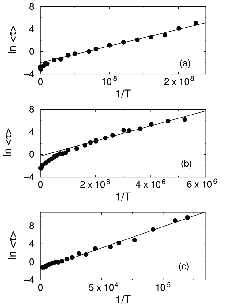
Figure 11: The average breaking time $\langle\tau\rangle$ required for the system to surmount the lowest energy barrier $\epsilon_{0}$ versus inverse temperature $1/T$ for three different MS packings with $N=10$ particles. The slope of the solid lines in panels (a)-(c) are $\epsilon_{0}\approx 3.3\times 10^{-8}$, $1.4\times 10^{-6}$, and $1.1\times 10^{-4}$.

IV.1.2 Measurement of energy barrier heights

In order to determine the height of the energy barrier that separates a given MS packing from other packings, we have performed a series of breaking-time measurements over a wide range of temperatures $T$. The simulations were performed on a randomly selected group of $105$ MS packings with $N=10$.

Measurements of the average minimal breaking time $\langle\tau\rangle$ versus the inverse temperature for three different MS packings are presented in Fig. 11. Each data point in these plots was obtained from an average of at least 20 independent measurements of the breaking time; the standard deviation of $\tau$ is comparable to the symbol size.

The results in Fig. 11 indicate that for sufficiently low temperatures the system exhibits Arrhenius behavior

$$\langle\tau\rangle=\tau_{\infty}e^{\epsilon_{0}/T}.$$ (11)

The quantity $\epsilon_{0}$ in the above relation is interpreted as the height of the energy barrier that separates a given MS packing from others. Below, both $\epsilon_{0}$ and $T$ will be measured in units of the characteristic energy scale $\epsilon$ of the repulsive spring potential in Eq. 1. The parameter $\tau_{\infty}$ characterizes the timescale at which the system explores the energy landscape.

We find from our results that the exponential behavior 11 is quite robust despite the fact that we use small systems with only $\sim 20$ translational degrees of freedom. The evolution occurs at constant energy with no heat reservoir—yet we observe pronounced thermal behavior. We note that the breaking time in the Arrhenius regime varies by several orders of magnitude, which allows us to determine the barrier height $\epsilon_{0}$ quite accurately.

At high temperatures, the MS packings break to a number of different destination MS packings because the system possesses enough kinetic energy to traverse a broad range of barriers. In the low-temperature regime, the system breaks by jumping over the lowest energy barrier, unless there are several barriers of nearly the same magnitude. By fitting the simulation data (such as those presented in Fig. 11) to the Arrhenius form 11 in the low-temperature regime we can thus measure the lowest energy barrier $\epsilon_{0}$ for each MS packing studied. At moderate temperatures, we can separately calculate the average breaking time $\langle\tau\rangle$ for each destination MS packing, which, in principle, allows us to measure the lowest, next lowest, and subsequent higher energy barriers.

Figure 12: The discrete probability $f_{k}$ with which a given MS packing occurs versus the lowest energy barrier $\epsilon_{0}$ associated with that packing using the (a) CG and (b) MD energy minimization methods. All $105$ MS packings in our sample are included. The filled circles correspond to the most probable set of MS packings $\{\mathcal{P}_{k}\}^{q=0.7}$, while the open circles indicate the remaining less frequent ones. The long-dashed line in panel (b) with slope $1.7$ points out the correlation between ${f}_{k}^{\rm MD}$ and $\epsilon_{0}$. The open square (cross) in both panels corresponds to the twin packing (meta-packing) discussed in Sec. IV.1.3.

IV.1.3 Relation between energy barriers an probabilities of MS packings

The Arrhenius plots presented in Fig. 11 reveal that the magnitudes of the minimal energy barriers $\epsilon_{0}$ separating distinct MS packings vary by many orders of magnitude. It is thus interesting to determine whether or not there is a relation between the energy-barrier heights and the MS packing probabilities ${f}_{k}$, which exhibit a similar large variation, as discussed in Sec. III. We have measured the energy-barrier heights for a sample of $105$ MS packings, which comprise only about $6.5\%$ of the total number of MS packings for the $10$-particle system considered (cf. the results in Table 1). The small sample size does not allow for a complete quantitative analysis of the problem, but we are able to make some interesting qualitative observations.

In Fig. 12 we compare the minimal energy barrier heights $\epsilon_{0}$ and the corresponding probabilities ${f}_{k}$ for our sample of MS packings. The probabilities shown in panel (a) were obtained using the CG protocol, and those depicted in panel (b) correspond to the MD algorithm. In both plots, the filled symbols indicate the data points for the packings in the set $\{\mathcal{P}_{k}\}^{q}$ of the most probable packings contributing to the truncated density of states $\rho_{q}(\phi)$ at the probability truncation level $q=0.70$. (The set $\{\mathcal{P}_{k}\}^{q}$ is defined near the end of Sec. III.2.3.) The open symbols correspond to less probable packings.

There are several interesting features to be noticed in these plots. In the case of the CG protocol, illustrated in Fig. 12(a), we see only a gross correlation between ${f}_{k}$ and $\epsilon_{0}$. The high-probability states tend to have high energy barriers, and the barriers of low-probability packings do not exceed $10^{-5}$ in our sample. Otherwise, the scatter in the data is very large; for example, the energy barriers of the packings in the probability range $10^{-4}$ to $10^{-3}$ vary by nearly ten orders of magnitude.

In contrast, there is a much stronger correlation between the probabilities and energy barriers in the subset of packings that have the maximal probability in each local packing-fraction region. We note that for a given value of ${f}_{k}$, the packings from the high-probability subset $\{\mathcal{P}_{k}\}^{q=0.7}$ (shown as filled circles in Fig. 12(a) ) tend to have the highest energy barriers $\epsilon_{0}$ for a given ${f}_{k}$.

The results presented in Fig. 12(b) show that the points in the high-probability subset are insensitive to the packing-generation protocol, consistent with the results shown in Fig. 9. However, the packings outside the subset $\{\mathcal{P}_{k}\}^{q=0.7}$ shift significantly in the low-probability direction when switching from the CG to MD method. Since packings outside $\{\mathcal{P}_{k}\}^{q=0.7}$ tend to have low energy barriers, the MD probabilities are much more strongly correlated with the heights of the minimal energy barriers than the CG probabilities. In fact, the data for the most probable states $\{\mathcal{P}_{k}\}^{q=0.7}$ in Fig. 12(b) roughly scale as a power-law ${f}_{k}^{\rm MD}\sim\epsilon_{0}^{\lambda}$ with $\lambda\approx 2$.

The above observations point out that the relationship between the probabilities of MS packings and $\epsilon_{0}$ is complex. On the one hand, the magnitude of the minimal energy barrier separating a given MS packing from other packings is not directly linked to the packing probability ${f}_{k}$, especially for the CG protocol. On the other hand, the energy-barrier heights clearly determine some important features of the probability distribution. In particular, the probabilities ${f}_{k}$ of MS packings with low energy barriers depend strongly on the packing-generation protocol, which can be seen by comparing the results in Figs. 12 (a) and (b). Moreover, there is a significant correlation between $\epsilon_{0}$ and ${f}_{k}$ for a subset of the most frequent packings for each $\phi$.

Strong protocol dependence of the probabilities ${f}_{k}$ for MS packings with low values of $\epsilon_{0}$ can be understood intuitively by noting that a system with weak but nonvanishing thermal fluctuations is able to surmount low energy barriers but not high ones. Thus for protocols such as the MD algorithm, the low-barrier packings tend to have low probabilities. After traversing the low barriers, the system becomes trapped in packings with higher barriers, which thus have higher probabilities.

We expect similar behavior to occur during the relaxation process of glass-forming liquids following a thermal quench. During the quench, the system first quickly relaxes by surmounting low energy barriers. At later times it evolves much more slowly through a set of high-barrier states, which is closely related to the high-probability subset $\{\mathcal{P}_{k}\}^{q}$ of MS packings. During the slow-evolution stage, the properties of the system are thus strongly affected by the truncated density of the most frequent states similar to the truncated density of MS packings $\rho_{q}(\phi)$ introduced in Fig. 9.

The large scatter of the data points in Fig. 12 indicates that additional geometrical features of the potential energy landscape—not simply the minimal energy barriers—must influence the probabilities of MS packings. Below we qualitatively discuss a few nonlocal topographic features that may play a significant role. A more detailed, quantitative investigation of such features is beyond the scope of the current study, but will be pursued in future work.

Figure 13: The packing fraction $\phi$ of the MS packing that is nearest to the instantaneous MD configuration at time $t$ for (a) a temperature comparable to the minimal energy-barrier height $T\sim\epsilon_{0}$ and (b) a temperature that is four times larger.

Twin packings and meta-packings

A relatively simple feature of the PEL that can give rise to significant fluctuations in the relation between the minimal energy barrier $\epsilon_{0}$ and the probabilities ${f}_{k}$ is illustrated in Fig. 13. This figure shows two sample breakup trajectories for the MS packing indicated by the open square in Fig. 12. The trajectory depicted in Fig. 13(a) corresponds to an initial thermal excitation with $T$ comparable to the minimal barrier height $\epsilon_{0}$; the trajectory depicted in Fig. 13(b) corresponds to a thermal excitation that is four times larger.

According to the results in Fig. 13, at the lower temperature the system oscillates between two MS packings that have nearly the same packing fraction $\phi$. We refer to these as twin packings. In order for the system to make a transition to a non-twin packing within this timescale, the temperature must be increased dramatically. After surmounting the barrier that takes the system to a non-twin packing, the system undergoes the usual cascade of transitions through a sequence of packings with increasing $\phi$ (cf. the trajectory depicted in Fig. 10).

The meta-packing that consists of the two twin packings between which the system oscillates at low temperatures can have a much higher energy barrier than the barrier $\epsilon_{0}$ separating the two component packings. We expect that the probability of the twin packings is controlled by the meta-packing energy barrier $\epsilon_{1}$ rather than the minimal barrier $\epsilon_{0}\ll\epsilon_{1}$. Thus, we have also included the data point $(\epsilon_{1},{f}_{k})$ for the twin-packing in Fig. 12 using a cross as the symbol. Note that using $\epsilon_{1}$ instead of $\epsilon_{0}$ brings this point closer to the cluster of data for the most probable subset of packings $\{\mathcal{P}_{k}\}^{q=0.7}$. A generalization of this picture to a larger group of packings will be carried out in a future publication future . When we perform this analysis we may likely find that more than two component packings can belong to a given meta-packing. We note that the concept of meta-packings is closely related to that of metabasins of the PEL debenedetti ; vogel .

Probability streams

Identifying neighboring packings that are separated by small energy barriers and grouping them into meta-packings may decrease the scatter of the data in Fig. 12, but it is unlikely to eliminate it. Thus, it is apparent that not only energy barriers but other geometric features of the PEL are important for determining the probabilities ${f}_{k}$. At present, we do not have any direct measurements of these additional features. However, our simulation results provide important clues that indicate directions for further investigations of the problem.

We may consider here two possibilities. First, one could assume that the volume $\Omega_{k}$ of the local region in configuration space with energy $V<\epsilon_{0}$ in the neighborhood of a given MS packing determines its probability ${f}_{k}$. For a given $\epsilon_{0}$, this volume may have large variations due to variations of the shape of the local potential-energy basin from one MS packing to another. However, as shown in Sec. IV.2 below, this possibility can be excluded since the multi-dimensional volume $\Omega_{k}$ depends too strongly on the height of the energy barrier.

Thus, a more complex, non-local scenario may better explain the MS packing probabilities. According to this scenario, the probability ${f}_{k}$ of a MS packing depends on two competing factors: the probability of getting into the neighborhood of that packing and the probability of leaving the local region before the MS packing is reached during the relaxation process. The probability of leaving the local region is largely controlled by the height of the energy barrier, and thus it is strongly protocol dependent. The probability of arriving into the neighborhood of an MS packing is affected by the size of the local region (therefore states from the high probability subset $\{\mathcal{P}_{k}\}^{q}$ tend to have high energy barriers), but it is more strongly influenced by the chain of events that brought the system into the neighborhood of the MS packing. These events, in turn, are determined by the features of PEL that can be far away from the local potential-energy basin for a given MS packing.

The large scatter in the probabilities for a given value of the energy barrier indicates that the flux of probability during the compaction process is very nonuniform. It appears that there are many “dry” regions, with very small probability flux, and “probability streams,” where the probability flux is very large. If a given MS packing is in the path of such probability streams, it may have a very large probability, even if the energy barrier $\epsilon_{0}$ associated with this packing is low.

We note that in our intuitive picture, probability flux is akin to water flow in a rugged mountainous landscape. This analogy, however, may be oversimplified due to the highly multidimensional character of the PEL for particulate systems.

Figure 14: Comparison of the eigenvalues of the displacement matrix $d_{i}/T$ for several temperatures $T$ (curves) and those of the inverse dynamical matrix $1/m_{i}$ (open squares) for (a) a system that has been compressed by $1\%$ from the jamming threshold and (b) a MS packing. Note that when plotting the eigenvalues of the dynamical and displacement matrices, we include only the $dN-d$ nontrivial eigenvalues and order them from smallest to largest.

IV.2 Displacement fluctuations

IV.2.1 Displacement and dynamical matrices

After a digression on possible non-local features of the PEL that can control the large fluctuations in the probabilities of MS packings, we now return to our analysis of local features of the PEL near a given MS packing. In this section we focus on measuring the shape and size of the local region visited by the system when the MS packing is thermally excited.

In general, the local shape of the PEL basin can be studied using both static and dynamic techniques. The static method relies on an analysis of the eigenvalue spectrum of the dynamical (Hessian) matrix 3 and 4. The dynamic technique that is applied in this section is based on the evaluation of the $2N$-dimensional matrix of displacements away from the reference MS packing while the system fluctuates after input of thermal energy. The displacement matrix is defined as

$$D_{i\alpha,j\beta}=\langle\left(r_{i\alpha}-r_{i\alpha 0}\right)\left(r_{j\beta}-r_{j\beta 0}\right)\rangle,$$ (12)

where $r_{i\alpha 0}$ are the coordinates of the reference MS packing, and $r_{i\alpha}$ are the current coordinates. Again, the indices $i$ and $j$ refer to the particles, and $\alpha,\beta=x,y$ represent the Cartesian coordinates. The average in Eq. 12 is taken both over times $t<\tau$ less than the minimal breaking time and over at least $20$ realizations at each $T$, weighted by the corresponding breaking time $\tau$.

In harmonic systems, the eigenvalues of the displacement matrix $d_{i}$ are trivially related to those of the dynamical matrix $m_{i}$

$$d_{i}=\frac{T}{m_{i}}.$$ (13)

Near an MS packing, however, our system of disks is strongly anharmonic, due to the one-sided character of the spring potential 1 at the jamming threshold. Thus, relation 13 is not guaranteed to hold even in the low-temperature limit.

Figure 15: (a) The minimum $d_{\rm min}$, (b) median $d_{\rm med}$, and (c) maximum $d_{\rm max}$ eigenvalues of the displacement matrix plotted versus the minimal energy-barrier height $\epsilon_{0}$ at temperature $T/\epsilon_{0}=0.2$ for $N=10$ and all $105$ packings in our sample. The eigenvalues of the displacement matrix scale as $d_{i}\sim\epsilon_{0}^{\gamma_{i}}$, and the power-law exponents $\gamma_{i}$ are given in Fig. 16. For $d_{\rm max}$, a few packings in the subset $\{\mathcal{P}_{k}\}^{q=0.7}$ (solid circles) deviate from the main trend.

We find that for compressed systems with finite particle overlaps there is a characteristic temperature $T_{c}$ below which relation 13 is satisfied. For example, a system compressed by $1\,\%$ above the jamming threshold behaves harmonically for $T<T_{c}\approx 10^{-5}$, as illustrated in Fig. 14(a). However, the temperature $T_{c}$ tends to zero as the amount of overlap decreases; therefore relation 13 is not valid for MS packings even at infinitesimal temperatures. The quantities on the left and right hand sides of Eq. 13 can differ by more than an order of magnitude for MS packings as shown in Fig. 14(b).

In what follows, we focus on the displacement matrix 12 (rather than the dynamical matrix) because it more reliably measures the local shape of potential energy landscape near MS packings. Moreover, at finite temperatures the matrix $D_{i\alpha,j\beta}$ yields information about the entire region of configuration space with energy $V<\epsilon_{0}$ near a given MS packing. Note that since we are considering thermally fluctuating systems in which all particles move, the distinction between rattler and non-rattler particles becomes less important and we will not distinguish between these two types of particles in the following discussion.

IV.2.2 Eigenvalues of displacement matrix

The results displayed in Fig. 14 (b) show that the eigenvalue spectrum of the displacement matrix for MS packings can be highly nonuniform. In this example, the ratio of the largest to smallest displacement eigenvalues $d_{\rm max}/d_{\rm min}$ is approximately $10^{3}$ at low temperatures. It is thus interesting to examine how this ratio, and more generally the shape of the basin near each MS packing, varies from one packing to another.

The shape of the local basins was explored by evaluating the displacement matrix 12 for different MS packings at a fixed value of $T/\epsilon_{0}$, so that for each packing we study comparable relative displacements away from potential energy minimum. We find that the eigenvalues of the displacement matrix exhibit power-law scaling with the energy-barrier height,

$$d_{i}\sim\epsilon_{0}^{\gamma_{i}},$$ (14)

where the scaling exponent $\gamma_{i}$ depends on the position $i$ in the set of $d(N-1)$ eigenvalues ordered by their magnitude.

Figure 16: The power-law exponents $\gamma_{i}$ that determine how the eigenvalues of the displacement matrix scale with the minimal energy-barrier height $\epsilon_{0}$. The index $i$ runs from the smallest eigenvalue of the displacement matrix to the largest. For harmonic systems, all $\gamma_{i}=1$.

The power-law behavior 14 is illustrated in Fig. 15 for the minimum, median, and maximum eigenvalues of the displacement matrix for $N=10$ at fixed $T/\epsilon_{0}=0.2$. We also performed measurements at $T/\epsilon_{0}=0.3$ and obtained similar results. The power-laws extend over at least $10$ orders of magnitude in $\epsilon_{0}$, although there is some scatter in the data for the largest eigenvalue $d_{\rm max}$. $d_{\rm max}$ for several of the packings from the most frequent subset $\{\mathcal{P}_{k}\}^{q=0.7}$ deviate from the main trend.

The scaling exponents are given in Fig. 16 and range from approximately $0.6$ for the largest eigenvalue to near $1.0$ for eigenvalues below the median. The fact that the largest several scaling exponents differ significantly from unity again indicates that MS packings are anharmonic, since in harmonic systems $\gamma_{i}=1$ (assuming that the eigenvalues of the dynamical matrix are independent of $\epsilon_{0}$).

Figure 17: Ratio $d_{\rm max}/d_{\rm min}$ of the maximum and minimum eigenvalues of displacement matrix versus the minimal energy-barrier height $\epsilon_{0}$ at temperature $T/\epsilon_{0}=0.2$ for $N=10$ and all $105$ packings in our sample. The long-dashed line has slope $-0.5$. The most frequent packings in the subset $\{\mathcal{P}_{k}\}^{q=0.7}$ are indicated by filled circles while the rest are indicated by open circles.

To illustrate the non-uniformity of the displacement-matrix spectrum, in Fig. 17 we plot the ratio $d_{\rm max}/d_{\rm min}$ versus $\epsilon_{0}$ at fixed $T/\epsilon_{0}=0.2$. We find that the ratio roughly obeys the power-law

$$\frac{d_{\rm max}}{d_{\rm min}}\sim\epsilon_{0}^{-0.5},$$ (15)

consistent with the results shown in Figs. 15 (a) and (c) and 16. Fig. 17 emphasizes that MS packings can possess extremely nonuniform displacement fluctuations with $d_{\rm max}/d_{\rm min}$ as large as $10^{7}$ for packings with small energy barriers. As in Fig. 15 (c), there are several frequent MS packings with $\epsilon_{0}<10^{-5}$ that have considerably larger ratios than this trend, but the vast majority of points obey (15).

Our data shows that MS packings possess highly nonuniform displacement eigenvalue spectra (nearly all have $d_{\rm max}/d_{\rm min}>100$) and the non-uniformity substantially increases with decreasing $\epsilon_{0}$. This suggests that the basins associated with MS packings are highly anisotropic in configuration space, and this gives rise to displacement fluctuations that are much larger in one or a few directions than others. Thus, one simple picture is that MS packings break only along particular directions in configuration space and that the breaking direction will be correlated with the direction in which the displacement fluctuations are the largest. We will investigate this intuitive picture in future studies.

The results presented in Figs. 15–17 allow us to determine if there is a direct link between the volume $\Omega_{k}$ and the packing probabilities ${f}_{k}$, where $\Omega_{k}$ is the volume of configuration space near a given MS packing that contains points with potential energy $V<\epsilon_{0}$ . An estimate of this volume can be obtained by assuming that at temperature $T\sim\epsilon_{0}$ the system explores a large portion of $\Omega_{k}$. Accordingly, we find

$$\Omega_{k}\sim\prod_{i=1}^{d(N-1)}\sqrt{d_{i}}\sim\epsilon_{0}^{\eta},$$ (16)

where $\eta=\frac{1}{2}\sum_{i=1}^{d(N-1)}\gamma_{i}$. The last expression in (16) was obtained using the relation between $d_{i}$ and $\epsilon_{0}$ in (14).

Thus, if we assume that the packing probabilities are controlled by the volume $\Omega_{k}$, we obtain

$${f}_{k}\sim\epsilon_{0}^{\eta},$$ (17)

where $\eta\approx 7$ for the $10$-particle system considered here. However, our results in Fig. 12 show that the dependence of the packing probabilities on $\epsilon_{0}$ is much weaker than that predicted by (17). The exponent for the $10$-particle data is approximately $2$, not $7$.

Thus, our results indicate that the packing probabilities are determined by a much lower dimensional quantity than the volume $\Omega_{k}$. Our results are consistent with a scenario in which the packing frequencies are determined by only the largest several displacement eigenvalues. It is likely that the packing probabilities are correlated with the largest displacement eigenvalues because they may correspond to the (initial) escape directions from the basin of a MS packing.

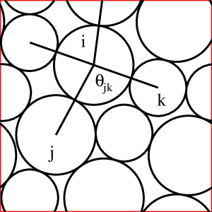
Figure 18: Definition of contact angles. $\theta_{jk}$ is the angle between the lines that connect the central particle $i$ to a pair of adjacent, contacting neighbors $j$ and $k$. There are four contact angles associated with particle $i$.

V Structural properties of MS packings

We also examined structural properties of MS packings in an attempt to identify features that control MS packing probabilities. Specifically, we measured the probability distributions for the angles between lines connecting centers of particles in contact (cf., the definition in Fig. 18). We focused on the distribution of maximal angles between particle contacts because large angles (close to $180^{\circ}$) correspond to unsupported (and thus unstable) chains of nearly collinear particles.

Figure 19: (a) Maximum contact angle $\theta_{\rm max}$ (in degrees) for each MS packing versus the frequency $f_{k}^{\rm MD}$ with which it occurs for a $10$-particle system using the MD energy minimization method. (b) The distribution of the largest contact angle $\theta^{i}_{\rm max}$ (in degrees) on each particle for the $100$ most frequent (thin lines) and $100$ most infrequent (thick lines) for the same system in (a). The dashed (solid) lines include all (larger half) $\theta^{i}_{\rm max}$ in each configuration.

As defined in Fig. 18, $\theta_{jk}$ is the angle between the lines connecting the central particle $i$ to pairs of adjacent, contacting neighbors $j$ and $k$. A given particle will possess $n_{c}$ contact angles, where $n_{c}$ is the number of contacts for that particle. We calculated the maximum contact angle $\theta^{i}_{\rm max}$ for each of the $N^{\prime}$ non-rattler particles and the maximum angle $\theta_{\rm max}$ for each configuration.

In Fig. 19 (a), we present a scatter plot of $\theta_{\rm max}$ for each MS packing in a system with $N=10$ particles versus the frequency ${f}_{k}$ with which the packing occurs for the MD packing-generation protocol. This plot shows that there is no strong correlation between $\theta_{\rm max}$ and ${f}_{k}$. In fact, some highly probable MS packings possess large contact angles near $180^{\circ}$.

Unsupported nearly linear chains of particles imply a low energy barrier. Since the barrier heights are correlated with the probability ${f}_{k}$ for the MD protocol, our results may thus suggest an important role of near contacts between particles. Such contacts do not directly support the chain but they may prevent transitions to other MS packings when the system is fluctuating donev_com . We will return to this problem in future investigations.

We also measured the distribution of the largest contact angles on each particle $\theta^{i}_{\rm max}$. In Fig. 19 (b), we compare the distributions of $\theta^{i}_{\rm max}$ for the $100$ most frequent (thin lines) and $100$ most infrequent (thick lines) MS packings generated for a $10$-particle system using the MD protocol. The figure shows two sets of curves. The probability distribution represented by the solid lines includes all $\theta^{i}_{\rm max}$ in the system; the dashed lines represent the distribution of only the largest half of the angles for each MS packing.

In contrast to the results represented in Fig. 19 (a), the distributions depicted in Fig. 19 (b) do show a clear correlation between large angles $\theta^{i}_{\rm max}$ and the frequencies ${f}_{k}$ of MS packings: The infrequent ones have an excess of large angles near $160^{\circ}$ compared to the frequent packings. Thus infrequent MS packings tend to have multiple particles with large contact angles.

The structural differences between the frequent and infrequent states that we see in Fig. 19 are quite subtle. We do not have any significant correlation with the single angle $\theta_{\rm max}$ in the packing. The differences show up, however, collectively in the distribution of the contact angles for each particle in the packing. One of our long-term goals is to connect important geometrical features of configuration space to structural properties of MS packings that can be measured in experiments.

VI Is there a hidden random variable?

In previous sections we presented a detailed study of the probability distribution of MS packings in small 2d systems of bidisperse frictionless disks. We showed that the probabilities of individual packings may differ by orders of magnitudes, not only as function of packing fraction, but also in individual narrow packing-fraction intervals. Moreover, we identified important features of the packing probabilities ${f}_{k}$ that are only weakly affected by the details of the packing-generation protocol.

Since our packing-generation algorithms do not target any specific packings, there must exist important properties of the multidimensional configuration space that give rise to such widely varying packing probabilities. We have examined several local properties of the PEL near the MS packing configurations and have found gross correlations between these properties and the packing probabilities. However, there is large statistical scatter in the data, and thus we conclude that none of the local features of PEL that we have examined can fully explain the packing probability distribution.

Yet, in spite of the complexity of the problem we have found several interesting regularities. In particular we have determined that the probabilities ${f}_{k}$ in a narrow packing-fraction interval, evaluated for different values of $N$, can be rescaled onto a single master curve with the characteristic shape shown in Fig. 6 (b). In this section we further explore this striking similarity of the sorted probability distributions. We base our analysis on a simple phenomenological model that has been inspired, in part, by the correlation between the packing probabilities and the minimal energy barriers [cf. Fig. 12 (b)].

In this model we characterize each MS packing by a set of $M$ independent continuous random variables

$$x_{1},\ldots,x_{M}>0,$$ (18)

all with the same probability distribution $\pi_{1}(x)$, which is approximately uniform for $x<x_{\rm max}$ and quickly decays beyond $x_{\rm max}$. The number of random variables $x_{k}$ is comparable to the number of degrees of freedom in the system $M=O(Nd)$. Our central assumption is that the probability ${f}_{k}$ of a MS packing within the packing-fraction interval of interest is controlled by the smallest of the random variables 18:

$${f}_{k}\sim\min(x_{1},\ldots,x_{M}).$$ (19)

Using this assumption, the probability density $\pi_{\rm min}$ for the random variable

$$y=\min(x_{1},\ldots,x_{M})$$ (20)

can be written as

$$\pi_{\rm min}(y) = M\pi_{1}(y)\Pi_{1}^{M-1}(y)$$ (21)

$$= -\frac{d}{dy}\Pi_{1}^{M}(y),$$

where

$$\Pi_{1}(y)=\int_{y}^{\infty}\pi_{1}(x)dx$$ (22)

is the probability that $x>y$.

From this result we can evaluate the expected value of the number of MS packings $k(\bar{y})$ that have $0<y<\bar{y}$,

$$\frac{k(\bar{y})}{k_{\rm max}}=\int_{0}^{\bar{y}}\pi_{\rm min}(y)dy=1-\Pi_{1}^{M}(\bar{y}),$$ (23)

where $k_{\rm max}$ is a total number of MS packings.

Now we apply the above results to the packing fraction interval in which we have $k_{\rm max}=n_{s}(\Delta\phi)$ states. After inserting assumption 19 into 23, we obtain the expression

$$\frac{k}{k_{\rm max}}=1-\Pi_{1}^{M}(a^{-1}{f}_{k}),$$ (24)

where $a$ is the proportionality constant in Eq. 19. Accordingly, for a given probability distribution $\Pi_{1}$, our analysis yields the relation between the sorted probabilities ${f}_{k}$ and the index $k$ in the sorted sequence of states. This relation corresponds to the plot shown in Fig. 6 (strictly speaking, to its inverse).

Our theory cannot be directly verified without specifying the distribution of the random variables $x_{k}$, and we do not have any a priori information regarding this distribution. Our goal here, therefore, is more limited. We simply want to determine whether or not the numerical results shown in Fig. 6 are consistent with our assumption that $\pi_{1}(x)$ is a relatively uniform function in some range of $x$, outside of which it quickly decays.

In making this assumption, we have in mind features of the PEL such as the distance from a given MS packing to the passes in the rim of the local potential-energy basin. In each direction, the distance to the rim is smaller than the particle diameter; it is also conceivable that the distance to the closest pass determines the probability ${f}_{k}$. However, the specific meaning of the hypothetical random variables 18 in our phenomenological theory at this point has not been fleshed out.

Figure 20: The right-hand side of Eq. 25 $(1-k/k_{\rm max})^{1/M}$, with $M=dN-d$, is plotted versus the normalized discrete packing frequencies ${f}_{k}/{f}_{k}^{\rm max}$ over the narrow packing fraction intervals in Fig. 6 using MS packings from the CG method in $N=10$ (dotted line), $12$ (long-dashed line), and $14$ (solid line) particle systems.

To determine the approximate form of the probability distribution $\Pi_{1}$ from our numerical results, relation 24 is inverted,

$$\Pi_{1}(a^{-1}{f}_{k})=\left(1-k/k_{\rm max}\right)^{1/M},$$ (25)

and the data sets represented in Fig. 6 are replotted in a form that emphasizes the structure of our model. Specifically, in Fig. 20, the quantity on the right-hand side of Eq. 25 is shown versus the normalized probability ${f}_{k}/{f}_{k}^{\rm max}$ approx . The results in Fig. 20 indicate that the transformed quantity 25 is a nearly linear function of ${f}_{k}$. By Eqs. 22 and 25, this linear behavior is consistent with

$$\pi_{1}(x)\sim\Theta(x),$$ (26)

where $\Theta(x)$ is the Heaviside step function. The form of the probability distribution $\pi_{1}$ determined from our numerical results is thus compatible with assumptions of our model.

The results in Fig. 20 cannot be treated as a direct verification of our model, and the model itself is rather ad hoc. Nevertheless, the simplicity of the result 26 is notable. We thus believe that our model captures at least some essential aspects of the problem. However, the exact source of the very broad distribution of the probabilities ${f}_{k}$ and the nature of the self-similarity of this distribution for different values of $N$ (as revealed by the results shown in Fig. 6) still remains an important open problem.

VII Conclusions and Future Directions

We have performed extensive numerical simulations with the aim of generating mechanically stable (MS) packings of frictionless disks in small bidisperse systems. The MS packings are created using a protocol in which we successively grow and shrink soft, purely repulsive particles. Each compression or decompression step is followed by potential energy minimization, until all particle overlaps are infinitesimal. We focus on small systems with at most $14$ particles in 2D because in these systems we are able to find nearly all distinct MS packings and can therefore accurately measure the frequency with which each packing occurs.

One of the principal results in this work is that MS packing frequencies differ by many orders of magnitude both as a function of packing fraction and within narrow packing-fraction intervals. We have implemented here a fairly generic algorithm for generating MS packings, and this algorithm does not specifically target any of them. Yet we find that packing frequencies are extremely varied; moreover, the frequency variation increases with system size. We also find that the probability distribution can be scaled onto a single master curve.

We argue that these striking results are important in a broader context of theories of jammed granular media and glassy materials. In thermodynamic theories for dense granular media mehta it is usually assumed that MS packings within a small packing-fraction interval are equally probable. For our packing-generation protocol, this assumption is certainly not valid. Although we do not yet have sufficient data, we believe that MS packings will also not be equally probable for other commonly used experimental protocols, e.g., slow shear majmudar or vibration under gravity nagel . However, thermodynamic theories based on the equal-probability assumption are often applied to understand the properties of sheared or vibrated granular materials makse2 ; barrat .

Our findings show that the often-used equal-probability assumption for stable grain packings in granular matter and inherent structures in glass-forming liquids should be re-examined. If it turns out that the assumption is generally violated, except for some unphysical, highly specialized algorithms (and we expect that this is the case), thermodynamic theories of disordered granular packings will need to be significantly reformulated.

In this work we focused entirely on a system of frictionless particles. However, we would like to point out that for frictional particles there is another conceptual difficulty with the assumption of equal-probability packings. Since static friction can arrest particle motion at different contact angles (analogous to a block that can stop at any position on a wedge) MS packings of frictional particles do not form points in configuration space, but rather continuous hyper-surfaces. Since packings of frictional particles are often hyperstatic force , the dimensionality of these hyper-surfaces changes from packing to packing, and it is thus difficult to introduce an appropriate probability measure.

Returning to the summary of the key results of our study, we note that important features of the MS packing probabilities do not change when we alter the packing-generation protocol. Thus, we argue that protocol-independent properties of configuration space must play an important role in determining the MS packing frequencies. To investigate the connection between geometric properties of configuration space and MS packing probabilities, we added thermal energy to a set of MS packings and then measured several quantities as the system fluctuated. We monitored the time that elapsed before a MS packing broke to a distinct one, which allowed us to determine the heights of energy barriers that separate one MS packing from another. We also studied the displacement fluctuations in all possible directions away from the original MS packing to infer crucial features of the shape of the basin near each packing.

We found a gross correlation between the frequencies ${f}_{k}$ of MS packings and the height of the lowest energy barrier $\epsilon_{0}$ separating this packing from other ones. The MD packing frequencies roughly scale as ${f}_{k}\sim\epsilon_{0}^{\lambda}$ with $\lambda\approx 2$, but there is significant scatter in the data. In addition, we found that the eigenvalues of the displacement matrix scale as $d_{i}\sim\epsilon_{0}^{\gamma_{i}}$ with $0.6\lesssim\gamma_{i}\lesssim 1$. These results suggest that the MS packing frequencies are determined by one or a few degrees of freedom, not by the local volume of configuration space near each basin (in which case ${f}_{k}$ would scale much more strongly with $\epsilon_{0}$). However, the scatter in our data implies that there are important unknown variables that are linked to the MS packing probabilities.

Our results clearly indicate that this is complex problem and much more work needs to be done to fully understand what determines the MS packing frequencies. Here we mention briefly some directions that we are actively pursuing to address this question. 1) We are measuring the hypervolumes of the regions in configuration space whose vertexes are the nearby low-order saddle points of each MS packing. We will investigate the relation between these hypervolumes and packing probabilities. 2) We are studying the ($dN-d$)-dimensional breaking vector that connects the initial MS packing to the MS packing to which it breaks. We want to determine whether or not the breaking vector is correlated with the directions of large displacements when the system is thermally fluctuating.

References

- (1) P. G. Debenedetti and F. H. Stillinger, Nature 410, 259 (2001).
- (2) X. Fu, D. A. Rigney, and M. L. Falk, J. Non-Cryst. Solids 317, 206 (2003).
- (3) F. Varnik, L. Bocquet, J.-L. Barrat, and L. Berthier, Phys. Rev. Lett. 90, 095702 (2003).
- (4) C. Maloney and A. Lemaître, Phys. Rev. Lett. 93, 195501 (2004).
- (5) A. Tanguy, J. P. Wittmer, F. Leonforte, and J.-L. Barrat, Phys. Rev. B 66, 174205 (2002).
- (6) M. D. Ediger, Annual Review of Physical Chemistry 51, 99 (2000).
- (7) F. H. Stillinger, Science 267, 1935 (1995).
- (8) M. S. Shell and P. G. Debenedetti, Phys. Rev. E 69, 051102 (2004).
- (9) E. LaNave, S. Mossa, and F. Sciortino, Phys. Rev. Lett. 88, 225701 (2002).
- (10) T. Keyes and J. Chowdhary, Phys. Rev. E 65, 041106 (2002).
- (11) S. Büchner and A. Heuer, Phys. Rev. E 60, 6507 (1999).
- (12) Z. W. Salsburg and W. W. Wood, J. Chem. Phys. 37, 798 (1962).
- (13) S. Sastry, T. M. Truskett, P. G. Debenedetti, S. Torquato, and F. H. Stillinger, Mol. Phys. 95, 289 (1998).
- (14) R. J. Speedy, J. Chem. Phys. 114, 9069 (2001).
- (15) R. J. Speedy, Biophys. Chem. 105, 411 (2003).
- (16) S. Torquato and F. H. Stillinger, J. Phys. Chem. B 105, 11849 (2001).
- (17) N. Xu, J. Bławzdziewicz, and C. S. O’Hern, Phys. Rev. E 71, 061306 (2005).
- (18) R. K. Bowles and R. J. Speedy, Physica A 262, 76 (1999).
- (19) R. K. Bowles and I. Saika-Voivod, Phys. Rev. E 73, 011503 (2006).
- (20) E. R. Weeks, J. C. Crocker, A. C. Levitt, A. Schofield, and D. A. Weitz, Science 287, 627 (2000).
- (21) E. R. Weeks and D. A. Weitz, Phys. Rev. Lett. 89, 095704 (2002).
- (22) B. Doliwa and A. Heuer, Phys. Rev. E 61, 6898 (2000).
- (23) D. Thirumalai and R. D. Mountain, Phys. Rev. E 47, 479 (1993).
- (24) H. Miyagawa, Y. Hiwatari, B. Bernu, and J. P. Hansen, J. Chem. Phys. 88, 3879 (1988).
- (25) A. Donev, F. H. Stillinger, and S. Torquato, “Do binary hard disks exhibit an ideal glass transition,” xxx.lanl.gov/cond-mat/0603183.
- (26) G. Adam and J. H. Gibbs, J. Chem. Phys. 43, 139 (1965).
- (27) J.-P. Bouchaud, J. de Physique I 2, 1705 (1992); C. Monthus and J.-P. Bouchaud, J. Phys. A: Math. Gen. 29, 3847 (1996).
- (28) C. S. O’Hern, S. A. Langer, A. J. Liu, and S. R. Nagel, Phys. Rev. Lett. 88, 075507 (2002).
- (29) C. S. O’Hern, L. E. Silbert, A. J. Liu, S. R. Nagel, Phys. Rev. E 68, 011306 (2003).
- (30) L. E. Silbert, D. Ertas, G. S. Grest, T. C. Halsey, and D. Levine, Phys. Rev. E 65, 031304 (2002).
- (31) H. A. Makse, D. L. Johnson, and L. M. Schwartz, Phys. Rev. Lett. 84, 4160 (2000); H. P. Zhang and H. A. Makse, Phys. Rev. E 72, 011301 (2005).
- (32) S. Torquato, T. M. Truskett, and P. G. Debenedetti, Phys. Rev. Lett. 84, 2064 (2000).
- (33) S. F. Edwards and R. B. S. Oakeshott, Physica A 157, 1080 (1989).
- (34) H. A. Makse and J. Kurchan, Nature 415, 614 (2002).
- (35) P. G. Debenedetti, F. H. Stillinger, T. M. Truskett, and C. J. Roberts, J. Phys. Chem. B 103, 7390 (1999).
- (36) J. G. Berryman, Phys. Rev. A 27, 1053 (1983).
- (37) A. Donev, S. Torquato, F. H. Stillinger, and R. Connelly, J. Applied Phys. 95, 989 (2004).
- (38) R. J. Speedy, J. Chem. Phys. 110, 4559 (1999).
- (39) W. H. Press, B. P. Flannery, S. A. Teukolsky, and W. T. Vetterling, Numerical Recipes in Fortran 77 (Cambridge University Press, New York, 1986).
- (40) S. Alexander, Phys. Rep. 296, 65 (1998).
- (41) We note that for there are a small number of rare MS packings that have been generated by the MD but not by the CG procedure.
- (42) We have set Boltzmann’s constant throughout.
- (43) S. Sastry, P. G. Debenedetti, and F. H. Stillinger, Nature 393, 554 (1998).
- (44) M. Vogel, B. Doliwa, A. Heuer, and S. C. Glotzer, J. Chem. Phys. 120, 4404 (2004).
- (45) F. H. Stillinger and T. A. Weber, J. Chem. Phys. 83, 4767 (1985).
- (46) G.-J. Gao, J. Bławzdziewicz, and C. S. O’Hern, unpublished.
- (47) We would like to acknowledge useful discussions with A. Donev on a related topic in hard-disk systems.
- (48) The index in the sorted probability data sets are discrete, and the probabilities correspond to a specific realization of a random variables 18. In contrast, the corresponding quantities in Eqs. 23–25 are average, continuous quantities. To approximately compensate for this discrepancy, we set , where is a fitting parameter that is used to adjust the position of the last few points on the high-probability end of the plots.
- (49) T. S. Majmudar and R. P. Behringer, Nature 435, 1079 (2005).
- (50) E. R. Nowak, J. B. Knight, E. Ben-Naim, H. M. Jaeger, and S. R. Nagel, Phys. Rev. E 57, 1971 (1998).
- (51) A. Barrat, J. Kurchan, V. Loreto, and M. Sellitto, Phys. Rev. Lett. 85, 5034 (2000); Phys. Rev. E 63, 051301 (2001).
- (52) T. Unger, J. Kertész, and D. E. Wolf, Phys. Rev. Lett. 94, 178001 (2005).