Josephson effect and quantum merging of two Bose superfluids

Abstract

We consider the Josephson effect when two independent Bose superfluids are weakly connected. In the presence of interparticle interaction and based on the calculations of the one-particle density matrix of the whole system, we find that the one-particle density matrix can be factorized which satisfies the general criterion of Bose superfluid proposed by Penrose and Onsager. By introducing an effective order parameter for the whole system, our researches show that there is Josephson effect for two independent Bose superfluids.

PACS: 67.40.-w; 67.40.Db; 32.80.Ys

I
introduction

In 1962, Brian Josephson predicted the Josephson effect Josephson by considering the quantum effect of two superconductors separated by a thin insulator. The Josephson effect is a natural quantum phenomenon for two coherently superposed macroscopic quantum objects. The subsequent experiments verified the Josephson effect and also lent support to the BCS theory about the physical mechanism of superconductors. The Josephson effect has been used in the invention of novel devices for extremely high-sensitivity measurements of currents, voltages, and magnetic fields. Up to date, there are still considerable interests in the fundamental physics and applications of this effect. Similarly to the case of superconductors, the ideal Josephson effect was also observed by investigating the flow of superfluid ${}^{4}He$ through an array of micro-apertures Helium . Recent experiments Albiez ; Anker also observed clear Josephson current and especially self-trapping phenomenon Smerzi for Bose condensates in dilute gases.

About twenty years ago, P. W. Anderson raised a famous question Anderson that when two initially separated superfluids are connected, whether the two superfluids would show a relative phase and therefore Josephson current. In the ordinary physical picture of Josephson effect, the initial quantum state is regarded as a coherent superposition of two macroscopic phase coherent quantum objects. In Anderson’s question, however, before connecting two superfluids, the two superfluids are completely independent. To answer Anderson’s question, we shall consider the problem that during the connection process or with the development of time after the connection process, whether the quantum state of the whole system will become a coherent superposition of two macroscopic quantum superfluids.

After the experimental realization of Bose-Einstein condensate in dilute gases BEC , there are a lot of interesting studies about the splitting of a condensate and merging of two independent condensates, which relate closely to the above Anderson’s question. The former question about the formation of a fragmented condensate during the splitting process of a condensate has been studied intensively Spekk ; Capuzzi ; Javan ; Menotti . The quantum merging of two independent condensates (i.e., the inverse process of the splitting) was also investigated recently by considering carefully the role of dissipation Zapata , and by considering both the adiabatic and nonadiabatic merging Yi based on the well-known two mode approximation Milburn . Most recently, the splitting and the following merging of an elongated condensate Mebrahtu is considered by including the finite-temperature effect. On the experimental side, a continuous condensate source was created by periodically replenishing a condensate with new condensates Chikk . This striking experiment also gives strong motivation to study theoretically the merging of independent condensates.

To describe the essential quantum feature of a Bose superfluid, Penrose and Onsager Penrose proposed the idea of off-diagonal long-range order (ODLRO) which gives the general criterion of a Bose superfluid. The ODLRO plays a very important role in the description of the Bose superfluid, especially because it has no classical analog Penrose ; Yang . For a single superfluid, if the one-particle density matrix $\langle\widehat{\Psi}^{\dagger}\left(\mathbf{r}_{1},t\right)\widehat{\Psi}\left(\mathbf{r}_{2},t\right)\rangle$ can be factorized, i.e., $\langle\widehat{\Psi}^{\dagger}\left(\mathbf{r}_{1},t\right)\widehat{\Psi}\left(\mathbf{r}_{2},t\right)\rangle=\Phi^{\ast}\left(\mathbf{r}_{1},t\right)\Phi\left(\mathbf{r}_{2},t\right)$, there is an ODLRO for the superfluid, and the superfluid can be regarded as a macroscopic quantum object which has stable spatial coherence property Penrose . For two initially independent superfluids, here we investigate theoretically the dynamic process of the whole system when the barrier separating two superfluids is decreased adiabatically so that the two initially separated and independent superfluids are weakly connected. Based on the calculations of the one-particle density matrix of the whole system, it is found that there is an interaction-induced quantum merging process for initially independent superfluids. After two initially independent superfluids merge into a single condensate, it is shown that $\langle\widehat{\Psi}^{\dagger}\left(\mathbf{r}_{1},t\right)\widehat{\Psi}\left(\mathbf{r}_{2},t\right)\rangle\simeq\Phi_{e}^{\ast}\left(\mathbf{r}_{1},t\right)\Phi_{e}\left(\mathbf{r}_{2},t\right)$ with $\Phi_{e}$ being an effective order parameter of the whole system. The effective order parameter has the property that it is a coherent superposition of two macroscopic wave functions. For weakly interacting Bose superfluids, we find that the evolution of $\Phi_{e}$ can be described very well by the ordinary Gross-Pitaevskii (GP) equation GP , and thus there is also Josephson current when two initially independent superfluids are weakly connected.

The paper is organized as follows. In Section II we introduce the effective order parameter of the whole system when the one-particle density matrix is calculated for the general situation. In Section III we give the expression of the overall energy and the evolution equations based on the action principle. A brief summary and discussion is given in Section IV.

II
effective order parameter for two initially independent Bose superfluids

For two independent Bose superfluids at zero temperature shown in Fig. 1a, the number of particles $N_{1}$ and $N_{2}$ in each of the two superfluids are fixed, and the corresponding quantum state is

$$\left|N_{1},N_{2}\right\rangle=\frac{C_{n}}{\sqrt{N_{1}!N_{2}!}}(\widehat{a}_{1}^{{\dagger}})^{N_{1}}(\widehat{a}_{2}^{{\dagger}})^{N_{2}}\left|0\right\rangle,$$ (1)

where $C_{n}$ is a normalization constant to assure $\left\langle N_{1},N_{2}|N_{1},N_{2}\right\rangle=1$. $\widehat{a}_{1}^{{\dagger}}$ ($\widehat{a}_{2}^{{\dagger}}$) is a creation operator which creates a particle described by the single-particle state $\phi_{1}$ ($\phi_{2}$) in the left (right) superfluid. In this initial quantum state, the quantum depletion is omitted. Thus, this initial quantum state is valid when $a/\overline{l}<<1$ with $a$ and $\overline{l}$ being respectively the scattering length and mean distance between particles. One should note that for two initially coherently-separated superfluids, the state is $\left|N\right\rangle=(\widehat{b}^{\dagger})^{N}\left|0\right\rangle/\sqrt{N!}$ with $\widehat{b}^{\dagger}$ being a creation operator which creates a particle with the single-particle state $\left(\sqrt{N_{1}}\phi_{1}+\sqrt{N_{2}}\phi_{2}\right)/\sqrt{N}$ with $N=N_{1}+N_{2}$. As shown in Fig. 1b, we consider the dynamic evolution process of the whole system when two initially independent superfluids are weakly connected.

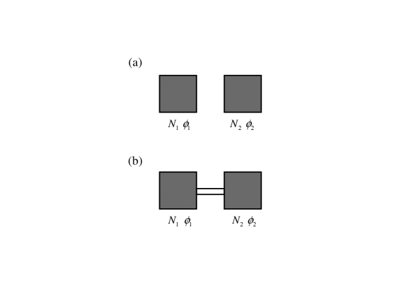
Figure 1: Shown in Fig. 1a is two independent Bose superfluids in two separate tanks. After the two Bose superfluids are connected shown in Fig. 1b, there is particle current between two tanks.

As shown in the following, after two independent Bose superfluids are connected, $\phi_{1}$ and $\phi_{2}$ will overlap and especially become non-orthogonal in the presence of interparticle interaction. Thus, we consider the general case for $\int\phi_{1}\phi_{2}^{\ast}dV=\zeta$ from the beginning. We first give the general expression of the one-particle density matrix $\langle\widehat{\Psi}^{\dagger}\left(\mathbf{x},t\right)\widehat{\Psi}\left(\mathbf{y},t\right)\rangle$ for this general case. Generally speaking, $\left|\zeta\right|<<1$. However, after straightforward calculations, it is shown clearly that the nonzero value of $\zeta$ can play important role in the one-particle density matrix for $N_{1}\left|\zeta\right|>1$ and $N_{2}\left|\zeta\right|>1$.

The operators $\widehat{a}_{1}$ and $\widehat{a}_{2}$ can be written as $\widehat{a}_{1}=\int\widehat{\Psi}\phi_{1}^{\ast}dV$ and $\widehat{a}_{2}=\int\widehat{\Psi}\phi_{2}^{\ast}dV$, respectively. Here $\widehat{\Psi}\left(\mathbf{x},t\right)$ is the field operator. By using the commutation relations of the field operators $[\widehat{\Psi}\left(\mathbf{x},t\right),\widehat{\Psi}\left(\mathbf{y},t\right)]=0$ and $[\widehat{\Psi}\left(\mathbf{x},t\right),\widehat{\Psi}^{\dagger}\left(\mathbf{y},t\right)]=\delta\left(\mathbf{x}-\mathbf{y}\right)$, it is easy to get the commutation relation $[\widehat{a}_{1},\widehat{a}_{2}^{\dagger}]=\zeta^{\ast}$. We see that $\widehat{a}_{1}$ and $\widehat{a}_{2}^{\dagger}$ are not commutative any more for $\int\phi_{1}\phi_{2}^{\ast}dV$ being a nonzero value.

It is well-known that the field operator should be expanded in terms of a complete and orthogonal basis set. Generally speaking, the field operator $\widehat{\Psi}\left(\mathbf{x},t\right)$ can be expanded as:

$$\widehat{\Psi}\left(\mathbf{x},t\right)=\widehat{a}_{1}\phi_{1}\left(\mathbf{x},t\right)+\widehat{k}\phi_{2}^{\prime}\left(\mathbf{x},t\right)+\cdots,$$ (2)

where $\phi_{1}$ and $\phi_{2}^{\prime}$ are orthogonal normalization wave functions. Assuming that $\phi_{2}^{\prime}=\beta\left(\phi_{2}+\alpha\phi_{1}\right)$, based on the conditions $\int\phi_{1}^{\ast}\phi_{2}^{\prime}dV=0$ and $\int\left|\phi_{2}^{\prime}\right|^{2}dV=1$, we have $\left|\beta\right|=\left(1-\left|\zeta\right|^{2}\right)^{-1/2}$ and $\alpha=-$ $\zeta^{\ast}$. Based on $\widehat{k}=\int\widehat{\Psi}\left(\phi_{2}^{\prime}\right)^{\ast}dV$, we have $\widehat{a}_{2}=\widehat{k}/\beta^{\ast}+\zeta\widehat{a}_{1}$.

Because $\widehat{k}$ and $\widehat{a}_{1}^{\dagger}$ are commutative, it is convenient to calculate the one-particle density matrix $\rho\left(\mathbf{x},\mathbf{y},t\right)$ using the operators $\widehat{k}$ and $\widehat{a}_{1}^{\dagger}$. The exact expression of $\rho\left(\mathbf{x},\mathbf{y},t\right)$ is

$$\rho\left(\mathbf{x},\mathbf{y},t\right) = \left\langle N_{1},N_{2},t\right|\widehat{\Psi}^{{\dagger}}\left(\mathbf{x},t\right)\widehat{\Psi}\left(\mathbf{y},t\right)\left|N_{1},N_{2},t\right\rangle$$ (3)

$$= \gamma_{1}\phi_{1}^{\ast}\left(\mathbf{x},t\right)\phi_{1}\left(\mathbf{y},t\right)+\gamma_{2}e^{i\varphi_{c}}\phi_{1}^{\ast}\left(\mathbf{x},t\right)\phi_{2}\left(\mathbf{y},t\right)$$

$$+\gamma_{2}e^{-i\varphi_{c}}\phi_{2}^{\ast}\left(\mathbf{x},t\right)\phi_{1}\left(\mathbf{y},t\right)+\gamma_{3}\phi_{2}^{\ast}\left(\mathbf{x},t\right)\phi_{2}\left(\mathbf{y},t\right),$$

where the coefficients are

$$\gamma_{1} = \sum\limits_{i=0}^{N_{2}}\frac{C_{n}^{2}N_{2}!\left(N_{1}+i-1\right)!N_{1}\left(1-\left|\zeta\right|^{2}\right)^{N_{2}-i}\left|\zeta\right|^{2i}}{i!i!\left(N_{1}-1\right)!\left(N_{2}-i\right)!},$$

$$\gamma_{2} = \sum\limits_{i=0}^{N_{2}-1}\frac{C_{n}^{2}N_{2}!\left(N_{1}+i\right)!\left(1-\left|\zeta\right|^{2}\right)^{N_{2}-i-1}\left|\zeta\right|^{2i+1}}{i!\left(i+1\right)!\left(N_{1}-1\right)!\left(N_{2}-i-1\right)!},$$

$$\gamma_{3} = \sum\limits_{i=0}^{N_{2}-1}\frac{C_{n}^{2}N_{2}!\left(N_{1}+i\right)!\left(1-\left|\zeta\right|^{2}\right)^{N_{2}-i-1}\left|\zeta\right|^{2i}}{i!i!N_{1}!\left(N_{2}-i-1\right)!}.$$ (4)

In addition, the normalization constant is determined by

$$C_{n}^{2}\left(\sum\limits_{i=0}^{N_{2}}\frac{N_{2}!\left(N_{1}+i\right)!\left(1-\left|\zeta\right|^{2}\right)^{N_{2}-i}\left|\zeta\right|^{2i}}{i!i!N_{1}!\left(N_{2}-i\right)!}\right)=1.$$ (5)

The phase factor $\varphi_{c}$ is determined by $\zeta=\left|\zeta\right|e^{i\varphi_{c}}$.

The above one-particle density matrix is obtained based on the second quantization method. We have also proven that this one-particle density matrix is equal to the result calculated from the many-body wave function which satisfies the exchange symmetry of identical bosons.

Introducing the ordinary order parameter $\Phi_{1}\left(\mathbf{x},t\right)=\sqrt{N_{1}}\phi_{1}\left(\mathbf{x},t\right)$ and $\Phi_{2}\left(\mathbf{x},t\right)=\sqrt{N_{2}}\phi_{2}\left(\mathbf{x},t\right)$, the one-particle density matrix can be naturally rewritten as

$$\rho\left(\mathbf{x},\mathbf{y},t\right)=\rho_{fac}\left(\mathbf{x},\mathbf{y},t\right)+\rho_{non}\left(\mathbf{x},\mathbf{y},t\right).$$ (6)

In the above equation, the factorable component $\rho_{fac}\left(\mathbf{x},\mathbf{y},t\right)$ is

$$\rho_{fac}\left(\mathbf{x},\mathbf{y},t\right)=\Phi_{e}^{\ast}\left(\mathbf{x},t\right)\Phi_{e}\left(\mathbf{y},t\right),$$ (7)

where we have introduced an effective order parameter

$$\Phi_{e}\left(\mathbf{x},t\right)=\sqrt{\gamma_{1}^{\prime}}\Phi_{1}\left(\mathbf{x},t\right)+\sqrt{\gamma_{3}^{\prime}}e^{i\varphi_{c}}\Phi_{2}\left(\mathbf{x},t\right).$$ (8)

The coefficients are $\gamma_{1}^{\prime}=\gamma_{1}/N_{1}$, $\gamma_{2}^{\prime}=\gamma_{2}/\sqrt{N_{1}N_{2}}$ and $\gamma_{3}^{\prime}=\gamma_{3}/N_{2}$. The non-factorable component $\rho_{non}\left(\mathbf{x},\mathbf{y},t\right)$ is

$$\rho_{non}\left(\mathbf{x},\mathbf{y},t\right)=\eta\left(e^{i\varphi_{c}}\Phi_{1}^{\ast}\left(\mathbf{x},t\right)\Phi_{2}\left(\mathbf{y},t\right)+e^{-i\varphi_{c}}\Phi_{2}^{\ast}\left(\mathbf{x},t\right)\Phi_{1}\left(\mathbf{y},t\right)\right),$$ (9)

where $\eta=\left(\gamma_{2}^{\prime}-\sqrt{\gamma_{1}^{\prime}\gamma_{3}^{\prime}}\right)$. We see that the parameter $\eta$ shows the proportion of the non-factorable component. If the coefficient $\eta$ is approximate to $0$, $\rho_{non}\left(\mathbf{x},\mathbf{y},t\right)$ can be omitted, and thus $\rho\left(\mathbf{x},\mathbf{y},t\right)$ can be approximated as the factorable component $\rho_{fac}\left(\mathbf{x},\mathbf{y},t\right)$.

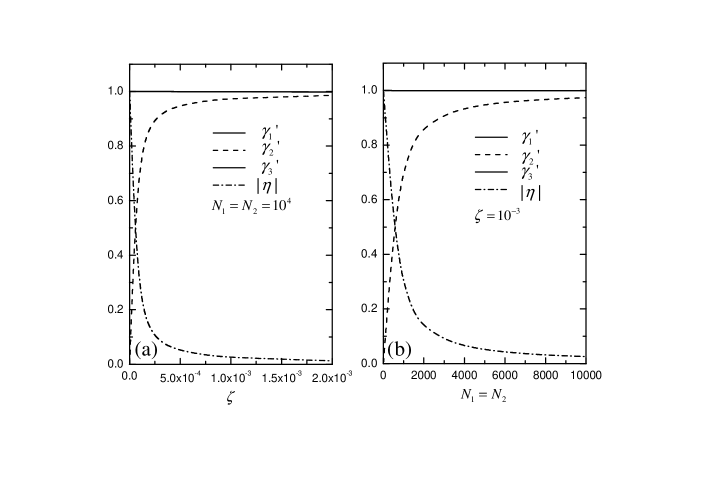
Figure 2: Proportion of the non-factorable component in the one-particle density matrix with different parameters. The relation between $\gamma_{1}^{\prime}$, $\gamma_{2}^{\prime}$, $\gamma_{3}^{\prime}$, $\left|\eta\right|$ and $\zeta$ for $N_{1}=N_{2}=10^{4}$ is shown in Fig. 2a, while the relation between $\gamma_{1}^{\prime}$, $\gamma_{2}^{\prime}$, $\gamma_{3}^{\prime}$, $\left|\eta\right|$ and $N_{1}=N_{2}$ for $\zeta=10^{-3}$ is shown in Fig. 2b. For the case of $N_{1}=N_{2}$, $\gamma_{1}^{\prime}=\gamma_{3}^{\prime}$. For $N_{1}\zeta>>1$, we have $\left|\eta\right|\approx 0$, thus the one-particle density matrix can be factorized in this situation.

For two initially independent and ideal superfluids, because $\zeta\left(t=0\right)=0$, based on the Schrődinger equation, it is easy to verify that $\zeta\left(t\right)=0$ at any further time. In this situation, $\rho\left(\mathbf{x},\mathbf{y},t\right)=\Phi_{1}^{\ast}\left(\mathbf{x},t\right)\Phi_{1}\left(\mathbf{y},t\right)+\Phi_{2}^{\ast}\left(\mathbf{x},t\right)\Phi_{2}\left(\mathbf{y},t\right)$. Obviously, $\rho\left(\mathbf{x},\mathbf{y},t\right)$ can not be factorized. Thus, the two superfluids can not be described by a single order parameter even there is an overlapping between two superfluids.

When the interparticle interaction is taken into account, however, $\zeta\left(t\right)$ can be a nonzero value. The nonzero value of $\zeta\left(t\right)$ physically arises from the interparticle interaction of the whole system. Although generally speaking, $\left|\zeta\left(t\right)\right|$ is much smaller than $1$ because $\phi_{1}\phi_{2}^{\ast}$ is an oscillation function about the space coordinate, it is easy to show based on Eq. (3) that a nonzero value of $\zeta\left(t\right)$ plays a very important role in the density matrix for large $N_{1}$ and $N_{2}$. As a general consideration, shown in Fig. 2a is the relation between $\gamma_{1}^{\prime}$, $\gamma_{2}^{\prime}$, $\gamma_{3}^{\prime}$, $\left|\eta\right|$ and $\zeta$ for $N_{1}=N_{2}=10^{4}$, while shown in Fig. 2b is the relation between $\gamma_{1}^{\prime}$, $\gamma_{2}^{\prime}$, $\gamma_{3}^{\prime}$, $\left|\eta\right|$ and $N_{1}=N_{2}$ for $\zeta=10^{-3}$. We see that when $N_{1}\left|\zeta\right|\sim 1$, the factorable component $\rho_{fac}\left(\mathbf{x},\mathbf{y},t\right)$ gives significant contribution to $\rho\left(\mathbf{x},\mathbf{y},t\right)$. In particular, when $N_{1}\left|\zeta\right|>>1$, one has $\left|\eta\right|\approx 0$, and thus the non-factorable component $\rho_{non}\left(\mathbf{x},\mathbf{y},t\right)$ can be omitted. In this situation, the one-particle density matrix can be factorized, and thus the whole system exhibits the property of ODLRO. According to the general criterion for Bose superfluid proposed by Penrose and Onsager, the factorability of the one-particle density matrix means that two initially independent superfluids have merged into a single superfluid which can be described by the effective order parameter $\Phi_{e}\left(\mathbf{x},t\right)$. After two independent superfluids merge into a single superfluid, we see that the relative phase $\varphi_{c}$ emerges naturally during the interaction-induced coherence process.

III overall energy and
dynamic evolution

We now turn to investigate the evolution equations of $\phi_{1}$ and $\phi_{2}$. The overall energy of the whole system is

$$E=\int dV\left\langle N_{1},N_{2},t\right|\left(-\frac{\hbar^{2}}{2m}\widehat{\Psi}^{{\dagger}}\nabla^{2}\widehat{\Psi}+V_{ext}\widehat{\Psi}^{{\dagger}}\widehat{\Psi}+\frac{g}{2}\widehat{\Psi}^{{\dagger}}\widehat{\Psi}^{{\dagger}}\widehat{\Psi}\widehat{\Psi}\right)\left|N_{1},N_{2},t\right\rangle,$$ (10)

where $g=4\pi\hbar^{2}a/m$ is the coupling constant with $a$ being the interparticle scattering length. $V_{ext}$ is the external potential of the system.

After straightforward calculations, the overall energy of the whole system is

$$E=E_{kin}+E_{pot}+E_{int},$$ (11)

where the kinetic energy $E_{kin}$ is given by

$$E_{kin} = \int\left\langle N_{1},N_{2},t\right|\frac{\hbar^{2}}{2m}\nabla\widehat{\Psi}^{{\dagger}}\cdot\nabla\widehat{\Psi}\left|N_{1},N_{2},t\right\rangle dV$$ (12)

$$= \int dV\left(\frac{\gamma_{1}\hslash^{2}}{2m}\nabla\phi_{1}^{\ast}\cdot\nabla\phi_{1}+\frac{\gamma_{2}\hbar^{2}}{2m}e^{i\varphi_{c}}\nabla\phi_{1}^{\ast}\cdot\nabla\phi_{2}\right.$$

$$\left.+\frac{\gamma_{2}\hbar^{2}}{2m}e^{-i\varphi_{c}}\nabla\phi_{2}^{\ast}\cdot\nabla\phi_{1}+\frac{\gamma_{3}\hbar^{2}}{2m}\nabla\phi_{2}^{\ast}\cdot\nabla\phi_{2}\right),$$

while the potential energy is given by

$$E_{pot} = \int\left\langle N_{1},N_{2},t\right|V_{ext}\widehat{\Psi}^{{\dagger}}\widehat{\Psi}\left|N_{1},N_{2},t\right\rangle dV$$ (13)

$$= \int V_{ext}\rho\left(\mathbf{r},\mathbf{r},t\right)dV.$$

In addition, the interaction energy $E_{int}$ of the whole system is given by

$$E_{int} = \int\left\langle N_{1},N_{2},t\right|\frac{g}{2}\widehat{\Psi}^{{\dagger}}\widehat{\Psi}^{{\dagger}}\widehat{\Psi}\widehat{\Psi}\left|N_{1},N_{2},t\right\rangle dV$$ (14)

$$= \frac{g}{2}\int dV\left[h_{1}\left|\phi_{1}\right|^{4}+h_{2}\left|\phi_{2}\right|^{4}+h_{3}\left|\phi_{1}\right|^{2}\left|\phi_{2}\right|^{2}\right.$$

$$\left.+\mathrm{Re}\left(h_{4}\left|\phi_{1}\right|^{2}\phi_{1}^{\ast}\phi_{2}e^{i\varphi_{c}}+h_{5}\left(\phi_{1}^{\ast}\right)^{2}\phi_{2}^{2}e^{2i\varphi_{c}}+h_{6}\left|\phi_{2}\right|^{2}\phi_{1}^{\ast}\phi_{2}e^{i\varphi_{c}}\right)\right],$$

where the coefficients are

$$h_{1} = \sum\limits_{i=0}^{N_{2}}\frac{C_{n}^{2}N_{2}!\left(N_{1}+i-2\right)!N_{1}\left(N_{1}-1\right)}{i!i!\left(N_{1}-2\right)!\left(N_{2}-i\right)!}\left(1-\left|\zeta\right|^{2}\right)^{N_{2}-i}\left|\zeta\right|^{2i},$$

$$h_{2} = \sum\limits_{i=0}^{N_{2}-2}\frac{C_{n}^{2}N_{2}!\left(N_{1}+i\right)!}{i!i!N_{1}!\left(N_{2}-i-2\right)!}\left(1-\left|\zeta\right|^{2}\right)^{N_{2}-i-2}\left|\zeta\right|^{2i},$$

$$h_{3} = \sum\limits_{i=0}^{N_{2}-1}\frac{4C_{n}^{2}N_{2}!\left(N_{1}+i-1\right)!N_{1}}{i!i!\left(N_{1}-1\right)!\left(N_{2}-i-1\right)!}\left(1-\left|\zeta\right|^{2}\right)^{N_{2}-i-1}\left|\zeta\right|^{2i},$$

$$h_{4} = \sum\limits_{i=0}^{N_{2}-1}\frac{4C_{n}^{2}N_{2}!\left(N_{1}+i-1\right)!N_{1}}{i!\left(i+1\right)!\left(N_{1}-2\right)!\left(N_{2}-i-1\right)!}\left(1-\left|\zeta\right|^{2}\right)^{N_{2}-i-1}\left|\zeta\right|^{2i+1},$$

$$h_{5} = \sum\limits_{i=0}^{N_{2}-2}\frac{2C_{n}^{2}N_{2}!\left(N_{1}+i\right)!}{i!\left(i+2\right)!\left(N_{1}-2\right)!\left(N_{2}-i-2\right)!}\left(1-\left|\zeta\right|^{2}\right)^{N_{2}-i-2}\left|\zeta\right|^{2i+2},$$

$$h_{6} = \sum\limits_{i=0}^{N_{2}-2}\frac{4C_{n}^{2}N_{2}!\left(N_{1}+i\right)!}{i!\left(i+1\right)!\left(N_{1}-1\right)!\left(N_{2}-i-2\right)!}\left(1-\left|\zeta\right|^{2}\right)^{N_{2}-i-2}\left|\zeta\right|^{2i+1}.$$ (15)

It is well known that the action principle is quite useful to derive the time-dependent GP equation for a single Bose superfluid. By using the ordinary action principle and the above overall energy, one can get the following coupled evolution equations for $\phi_{1}$ and $\phi_{2}$:

$$i\hslash\frac{\partial\phi_{1}}{\partial t} = \frac{1}{N_{1}}\frac{\delta E}{\delta\phi_{1}^{\ast}},$$

$$i\hslash\frac{\partial\phi_{2}}{\partial t} = \frac{1}{N_{2}}\frac{\delta E}{\delta\phi_{2}^{\ast}},$$ (16)

where $\delta E/\delta\phi_{1}^{\ast}$ and $\delta E/\delta\phi_{2}^{\ast}$ are functional derivatives.

Although the coupled evolution equations (16) are quite complex, for the case of $N_{1}\left|\zeta\right|>>1$, $N_{2}\left|\zeta\right|>>1$ and $N_{1}\sim N_{2}$, there is a very concise approximate evolution equation. When these conditions are satisfied, the overall energy of the whole system can be approximated very well as

$$E_{app}^{\prime}=E_{kin}^{\prime}+E_{pot}^{\prime}+E_{int}^{\prime},$$ (17)

where

$$E_{kin}^{\prime}=\frac{\hbar^{2}}{2m}\int\nabla\Phi_{e}^{\ast}\cdot\nabla\Phi_{e}dV,$$ (18)

$$E_{pot}^{\prime}=\int V_{ext}\left|\Phi_{e}\right|^{2}dV,$$ (19)

$$E_{int}^{\prime}=\frac{g}{2}\int dV\left|\Phi_{e}\right|^{4}.$$ (20)

For the cases of $N_{1}\left|\zeta\right|>>1$, $N_{2}\left|\zeta\right|>>1$ and $N_{1}\sim N_{2}$, it is easy to verify that $E_{kin}^{\prime}\approx E_{kin}$ and $E_{pot}^{\prime}\approx E_{pot}$ based on the analogous analyses about the effective order parameter that $\rho\left(\mathbf{x},\mathbf{y},t\right)\approx\Phi_{e}^{\ast}\left(\mathbf{x},t\right)\Phi_{e}\left(\mathbf{y},t\right)$ in this situation. For $N_{1}\left|\zeta\right|>>1$, $N_{2}\left|\zeta\right|>>1$ and $N_{1}\sim N_{2}$, one can also prove the result of $E_{int}^{\prime}\approx E_{int}$. Based on Eq. (20), $E_{int}^{\prime}$ can be expanded as:

$$E_{int}^{\prime} = \frac{g}{2}\int dV\left[\beta_{1}\left|\phi_{1}\right|^{4}+\beta_{2}\left|\phi_{2}\right|^{4}+\beta_{3}\left|\phi_{1}\right|^{2}\left|\phi_{2}\right|^{2}\right.$$ (21)

$$\left.+\mathrm{Re}\left(\beta_{4}\left|\phi_{1}\right|^{2}\phi_{1}^{\ast}\phi_{2}e^{i\varphi_{c}}+\beta_{5}\left(\phi_{1}^{\ast}\right)^{2}\phi_{2}^{2}e^{2i\varphi_{c}}+\beta_{6}\left|\phi_{2}\right|^{2}\phi_{1}^{\ast}\phi_{2}e^{i\varphi_{c}}\right)\right],$$

where

$$\beta_{1} = \gamma_{1}^{2},$$

$$\beta_{2} = \gamma_{3}^{2},$$

$$\beta_{3} = 4\gamma_{1}\gamma_{3},$$

$$\beta_{4} = 4\gamma_{1}\sqrt{\gamma_{1}\gamma_{3}},$$

$$\beta_{5} = 2\gamma_{1}\gamma_{3},$$

$$\beta_{6} = 4\gamma_{3}\sqrt{\gamma_{1}\gamma_{3}}.$$ (22)

To compare with the exact expression of the interaction energy given by Eq. (14), Fig. 3 shows the relation between $h_{i}/\beta_{i}$ ($i=1,\cdots,6$) and $\zeta$ for $N_{1}=N_{2}=10^{3}$. It is shown clearly that for $N_{1}\left|\zeta\right|>>1$ and $N_{2}\left|\zeta\right|>>1$, $h_{i}/\beta_{i}\approx 1$, and thus $E_{int}^{\prime}\approx E_{int}$.

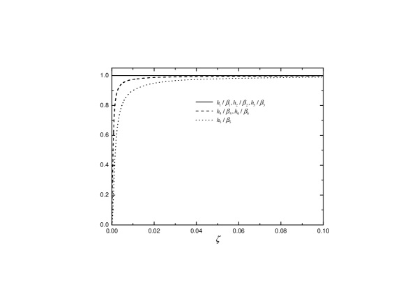
Figure 3: Shown is the relation between $h_{i}/\beta_{i}$ ($i=1,\cdots,6$) and $\zeta$ for $N_{1}=N_{2}=10^{3}$. We see that for $N_{1}\left|\zeta\right|>>1$ and $N_{2}\left|\zeta\right|>>1$, $h_{i}/\beta_{i}\approx 1$, which means that $E_{int}^{\prime}\approx E_{int}$.

Therefore, the overall energy can be approximated well as

$$E\simeq-\frac{\hbar^{2}}{2m}\int\Phi_{e}^{\ast}\nabla^{2}\Phi_{e}dV+\int V_{ext}\left|\Phi_{e}\right|^{2}dV+\frac{g}{2}\int dV\left|\Phi_{e}\right|^{4},$$ (23)

where $\Phi_{e}\left(\mathbf{x},t\right)$ is the effective order parameter given by Eq. (8). Based on this approximate energy expression, it is easy to get the following evolution equation for $\Phi_{e}\left(\mathbf{x},t\right)$:

$$i\hslash\frac{\partial\Phi_{e}}{\partial t}\simeq-\frac{\hslash^{2}}{2m}\nabla^{2}\Phi_{e}+V_{ext}\Phi_{e}+g\left|\Phi_{e}\right|^{2}\Phi_{e}.$$ (24)

It is quite interesting to note that the above equation has the same form as the standard GP equation GP .

Because there is no exact analytic solution for Eq. (16), here we give the solution based on numerical calculations. We consider the one-dimensional dynamic process when two initially independent condensates in dilute atomic gases are weakly connected through adiabatically decreasing the height of the barrier separating two condensates. The time-dependent double-well potential is assumed as

$$V_{ext}\left(x,t\right)=\frac{1}{2}m\omega_{x}^{2}x^{2}+U\left(t\right)e^{-x^{2}/\Delta_{x}^{2}},$$ (25)

where $U\left(t\right)=U_{0}e^{-\theta t}+U_{1}$. The first term is the external potential due to a magnetic trap or an optical trap, while the second term is the central barrier due to a laser beam separating two condensates. When the central barrier separating two condensates is sufficiently high so that there is no tunneling current, one may prepare two completely independent (rather than coherently separated) condensates by directly cooling the dilute gases in the double-well trap. In the last ten years, the remarkable experimental advances BEC on Bose condensate in dilute gases make it be quite promising to experimentally test the theoretical predication in this work.

In the numerical calculations, we introduce the dimensionless parameters $x_{0}=x/l_{x}$, $\tau=E_{l}t/\hslash$, $g^{\prime}=g/E_{l}l_{x}$. Here $l_{x}=\sqrt{\hslash/m\omega_{x}}$ and $E_{l}=\hbar^{2}/2ml_{x}^{2}$. The particle number is $N_{1}=2\times 10^{4}$ and $N_{2}=10^{4}$. In addition, $U_{0}=400E_{l}$, $U_{1}=20E_{l}$, $\theta=2E_{l}/\hbar$, $\Delta_{x}=l_{x}$ and $g^{\prime}N_{1}=50$. For these parameters, the tunneling effect can be omitted for two independent condensates at the initial time. When the central barrier due to the laser beam is decreased, there is particle current between two condensates.

In the numerical calculations, first we get the ground state wave functions $\phi_{1}$ and $\phi_{2}$ at the initial time. Then, by numerically calculating the coupled equations (16), we obtain the evolution of $\zeta\left(t\right)$ based on the numerical results of $\phi_{1}$ and $\phi_{2}$. From $\zeta\left(t\right)$, we give the evolution of $\left|\eta\right|$ in Fig.4. We have also confirmed in the numerical calculations that, for $g^{\prime}=0$, the numerical result of $\left|\zeta\right|$ can be regarded as zero because it is smaller than $10^{-10}$. This shows clearly that the nonzero value of $\left|\zeta\right|$ physically arises from the interatomic interaction, rather than the error in the numerical calculations. In fact, if we assume that $\zeta\left(t\right)$ is always zero with the development of time, it is easy to show that this is an inconsistent assumption because with this assumption we prove both in the numerical calculations and analytic analysis that $\left|\zeta\right|$ will increase from zero after the overlapping between two condensates. In the inset of Fig.4, we give the numerical result of $N_{1}\left(t\right)/N$ which shows clearly the Josephson effect. Our numerical results show that $\left(N_{1}\left(t\right)+N_{2}\left(t\right)\right)/N$ is always equal to $1$ with an error below $10^{-11}$ which confirms further our numerical calculations.

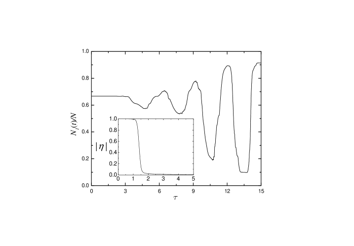
Figure 4: Quantum merging process shown through the evolution of $\left|\eta\right|$ and the Josephson effect. The evolution of $N_{1}/N$ shows clearly the Josephson effect. Due to the particle current between two initially independent condensates, as shown in the inset, $\left|\eta\right|$ decreases significantly with the development of time. At $\tau>3$, $\left|\eta\right|\approx 0$, thus two initially independent condensates have merged into a single condensate.

Although the Josephson effect shown in Fig.4 is the numerical results of Eq. (16), one can understand easily this effect with the effective order parameter. Due to the quantum merging process, when the central barrier separating two independent condensates is decreased, two initially independent condensates will merge into a single condensate described by the effective order parameter $\Phi_{e}$ whose evolution is determined by GP equation (24). Thus, it is natural that there is coherent Josephson current for two initially independent interacting condensates.

IV
summary and discussion

In summary, we investigate the dynamic process of the whole system when the barrier separating two initially independent Bose superfluids is adiabatically decreased so that the two initially separated and independent superfluids are weakly connected. When the interparticle interaction is considered, we show that there is an effective order parameter for the whole system under appropriate condition. Compared with previous interesting studies Zapata ; Yi ; Mebrahtu about quantum merging, in the present work, we consider this problem by stressing the non-orthogonal property between the wave functions for different condensates after their overlapping and in the presence of interparticle interaction. In particular, it is found that the effective order parameter satisfies the ordinary Gross-Pitaevskii equation, which means that there is also Josephson effect for two initially independent Bose superfluids. This result for the effective order parameter makes our theory can be tested and applied directly in future experiments about quantum merging process, such as the experiment about Josephson effect for independent Bose superfluids.

We stress here again that, in our theory, the quantum depletion originating from the elementary excitations at zero temperature is omitted in the initial state (1). Based on the Bogoliubov theory of the elementary excitations Pethick , the number of particles due to the elementary excitations is of the order of $\left(a/\overline{l}\right)^{3/2}$ and thus the quantum depletion is negligible for Bose condensate in dilute gases. There is another reason why the elementary excitations can be omitted in the effective order parameter. A simple analysis shows that $\left\langle\phi_{1}|\phi_{k}\right\rangle$ and $\left\langle\phi_{2}|\phi_{k}\right\rangle$ (here $\phi_{k}$ is the normalized wave function of the elementary excitations) are of the order of $\left|\zeta\right|e^{-(k-2\pi/L)^{2}}$ with $k$ and $L$ being respectively the wave number of the elementary excitations and spatial size of the Bose superfluid. This exponential decay of $\left\langle\phi_{1}|\phi_{k}\right\rangle$ and $\left\langle\phi_{2}|\phi_{k}\right\rangle$ originates from the integral where there is spatially oscillating phase factor in the wave functions of the elementary excitations and Bose superfluid. Thus, even there are elementary excitations, its contribution to the effective order parameter is negligible. Although the present theory can not give quantitative predication for liquid superfluid of ${}^{4}\mathrm{He}$ because the quantum depletion is very important, we believe that the quantum merging process means that after two separate tanks are connected by a pipe, two superfluids of ${}^{4}\mathrm{He}$ can merge into a single superfluid.

For the quantum state given by Eq. (1), with the development of time, the wave functions $\phi_{1}$ and $\phi_{2}$ are no more orthogonal in the presence of interparticle interaction. If we use the orthogonal bases $\phi_{1}$ and $\phi_{2}^{\prime}$, the quantum state of the whole system is $\left|N_{1},N_{2}\right\rangle\sim(\widehat{a}_{1}^{{\dagger}})^{N_{1}}(\widehat{k}/\beta^{\ast}+\zeta\widehat{a}_{1})^{N_{2}}\left|0\right\rangle$. We see that the number of particles in the orthogonal modes $\phi_{1}$ and $\phi_{2}^{\prime}$ are no more definite. This quantum state becomes a superposition of different number of particles in the orthogonal modes $\phi_{1}$ and $\phi_{2}^{\prime}$. This implies strongly that in some sense our theory is equivalent to the Gutzwiller type approach Gutzwiller where the coupling between different modes leads to the coherent transfer of particles between different orthogonal modes.

It is straightforward to generalize the present work to the quantum merging process of several independent Bose superfluids. It is possible that this quantum merging process contributes to our understanding of the Bose condensation process. During the evaporative cooling process, firstly there would be a series of independent subcondensates formed from the thermal cloud. Due to the quantum merging process, these independent subcondensates will overlap and finally merge into a single condensate with well spatial coherence property. During the evaporative cooling process, due to the thermal equilibrium of the whole system, the thermal atoms continuously jump into the ground state. The quantum merging process has the effect that the atoms in the ground sate merge into a single condensate which has well spatial and phase coherence property.

References

• (1) B. D. Josephson, Phys. Lett. 1, 251 (1962).
• (2) K. Sukhatme, Y. Mukharsky, T. Chui, and D. Pearson, Nature 411, 280 (2001).
• (3) M. Albiez, R. Gati, J. FΕ‘lling, S. Hunsmann, M. Cristiani, and M. K. Oberthaler, Phys. Rev. Lett. 95, 010402 (2005).
• (4) Th Anker, M. Albiez, R. Gati, S. Hunsmann, B. Eiermann, A. Trombettoni, and M. K. Oberthaler, Phys. Rev. Lett. 94, 020403 (2005).
• (5) A. Smerzi, S. Fantoni, S. Giovanazzi, and S. R. Shenoy, Phys. Rev. Lett. 79, 4950 (1997).
• (6) P. W. Anderson, in The Lesson of Quantum Theory, J. D. Boer, E. Dal, O. Ulfbeck, Eds. (Elsevier, Amsterdam 1986), pp. 23–33.
• (7) For review, see special issue Nature Insight: Ultracold Matter, Nature 416, 205 (2002).
• (8) R. W. Spekkens, and J. E. Sipe, Phys. Rev. A 59, 3868 (1999).
• (9) P. Capuzzi, and E. S. HernΓ‘ndez, Phys. Rev. A 59, 3902 (1999).
• (10) Juha Javanainen, and Misha Yu. Ivanov, Phys. Rev. A 60, 2351 (1999).
• (11) C. Menotti, J. R. Anglin, J. I. Cirac, and P. Zoller, Phys. Rev. A 63, 023601 (2001).
• (12) I. Zapata, F. Sols, and A. J. Leggett, Phys. Rev. A 67, 021603(R) (2003).
• (13) W. Yi, and L. -M. Duan, Phys. Rev. A 71, 043607 (2005).
• (14) G. J. Milburn, J. Corney, E. M. Wright, and D. F. Walls, Phys. Rev. A 55, 4318 (1997).
• (15) A. Mebrahtu, A. Sanpera, and M. Lewenstein, Phys. Rev. A 73, 033601 (2006).
• (16) A. P. Chikkatur, Y. Shin, A. E. Leanhardt, D. Kielpinski, E. Tsikata, T. L. Gustavson, D. E. Pritchard, and W. Ketterle, Science 296, 2193 (2002).
• (17) O. Penrose, L. Onsager, Phys. Rev. 104, 576 (1956).
• (18) C. N. Yang, Rev. Mod. Phys. 34, 694 (1962).
• (19) E. P. Gross, Nuovo Cimento 20, 454 (1961); J. Math. Phys. 4, 195 (1963); L. P. Pitaevskii, Zh. Eksp. Teor. Fiz. 40, 646 (1961) [Sov. Phys.-JETP 13, 451 (1961)].
• (20) C. J. Pethick and H. Smith, Bose-Einstein Condensation in Dilute Gases (Cambridge University, Cambridge, 2002).
• (21) M. C. Gutzwiller, Phys. Rev. 137, A1726 (1965).