Random field Ising model on networks with inhomogeneous connections

Abstract

We study a zero-temperature phase transition in the random field Ising model on scale-free networks with the degree exponent $\gamma$. Using an analytic mean-field theory, we find that the spins are always in the ordered phase for $\gamma<3$. On the other hand, the spins undergo a phase transition from an ordered phase to a disordered phase as the dispersion of the random fields increases for $\gamma>3$. The phase transition may be either continuous or discontinuous depending on the shape of the random field distribution. We derive the condition for the nature of the phase transition. Numerical simulations are performed to confirm the results.

I introduction

Recently physicists have recognized that the underlying graphs or networks for interacting systems have an intriguing structure. Such complex networks are distinct from the periodic lattices in Euclidean space in many aspects. The structural property of the complex networks has been studied intensively Albert2002 ; Newman2003a ; Dorogovtsev2001a . Besides the network topology itself, traditional topics of statistical physics of complex networks have been investigated as well Pekalski2001 ; Hong2002 ; BJKim2001 ; Lopes2004 ; DJeong2005 ; Sood2004a ; Goltsev03 ; Dorogovtsev04 ; Igloi2002 ; Michard2005 ; SWSon2005 . Statistical physical systems of networks are attractive since they display theoretically interesting critical phenomena Goltsev03 ; Dorogovtsev04 ; Igloi2002 . They are also attractive for a possible application to various phenomena in social systems having a complex underlying network structure  Sood2004a ; Michard2005 ; SWSon2005 .

In contrast to the periodic lattices in Euclidean space, complex networks have an inhomogeneous structure. Recent studies reveal that the structural inhomogeneity plays an important role in critical phenomena on complex networks Sood2004a ; Goltsev03 ; Dorogovtsev04 ; Igloi2002 ; Satorras2001 ; Catanzaro2004 . However, in the study of the critical phenomena, systems with quenched disorder have received little attention with only a few exceptions DHKim2005 ; Mooij2004 . In this work we investigate the effect of quenched disorder and structural inhomogeneity on the nature of a phase transition. For this purpose, we study a disorder-driven phase transition in the random field Ising model (RFIM) on scale-free (SF) networks. A SF network is characterized by the power-law degree distribution $P_{d}(k)\sim k^{-\gamma}$ with the degree exponent $\gamma$. The power-law distribution indicates that SF networks have an inhomogeneous structure and the degree exponent $\gamma$ determines the strength of the inhomogeneity in structure.

The RFIM has attracted much attention in statistical physics Schneider1977 ; Aharony1978 ; Villain1984 ; Bruinsma1984 ; Imbrie1984 ; Newman1996 ; Middleton2002 ; Swift1997 ; dAuriac1997 . Being compared with the spin glass model where the quenched disorder is present in the interaction among spins MezardBook , the RFIM has a quenched random external magnetic field applied to each site. The quenched disorder leads to a phase transition from an ordered ferromagnetic phase to a disordered paramagnetic phase. In spite of the simpler structure of the RFIM than the spin glass model, there are still remaining questions and controversies, especially over the nature of the phase transition Schneider1977 ; Aharony1978 ; Villain1984 ; Bruinsma1984 ; Imbrie1984 ; Newman1996 .

We study the zero-temperature phase transition in the RFIM using an analytic mean-field theory. Our analysis shows that the shape of the random field distribution and the degree exponent $\gamma$ determine the nature of the disorder-driven phase transition. We also perform numerical simulations, which confirm the analytic results. This paper is organized as follows: In Sec. II, an analytic approach based on mean-field theory and its prediction of the phase transition nature are provided. Numerical simulations follow in Sec. III, and Sec. IV summarize our work.

II analytic mean-field theory

The Hamiltonian of the RFIM on a network is given by

$$\mathcal{H}=-J\sum_{i<j}a_{ij}s_{i}s_{j}-\sum_{i}h_{i}s_{i},$$ (1)

where $s_{i}=\pm 1$ is the Ising spin variable of node $i=1,2,\ldots,N$, $J>0$ is the ferromagnetic coupling strength between neighboring spins, and $a_{ij}$ is the adjacency matrix element of the network. The matrix element $a_{ij}$ takes the value of $1~{}(0)$ if two nodes $i$ and $j$ are (not) connected via a link. The degree of a node $i$ is given by $k_{i}=\sum_{j}a_{ij}$. We will set $J=1$ hereafter for notational simplicity. Here the external magnetic field $h_{i}$ is a quenched random variable, which is distributed identically and independently according to a distribution function $p(h)$. We only consider a symmetric distribution – that is, $p(h)=p(-h)$. It is convenient to write

$$p(h)=\frac{1}{\Delta}p_{0}\Big{(}\frac{h}{\Delta}\Big{)},$$ (2)

where $p_{0}(x)$ is a normalized [$\int p_{0}(x)dx=1$] function determining the shape of the distribution and $\Delta$ is a measure of the disorder strength.

The ferromagnetic coupling $J$ favors the ordered state with all spins up or down. The external magnetic field, however, tends to pin each spin to a random direction. The competition between them may lead to a phase transition, which will be investigated at zero temperature using mean-field theory. In the framework of the mean-field theory, each spin $s_{i}$ is assumed to be in equilibrium under the effective magnetic field $\tilde{h_{i}}\equiv\sum_{j}a_{ij}m_{j}+h_{i}$ where $m_{j}\equiv\langle s_{j}\rangle$ is the average local magnetization at node $j$. Hence, the average local magnetization should satisfy the coupled mean-field equation

$$m_{i}=\langle s_{i}\rangle=\tanh\left(\beta\sum_{j}a_{ij}m_{j}+\beta h_{i}\right),$$ (3)

where $\beta=1/(k_{B}T)$ with the Boltzmann constant $k_{B}$ and temperature $T$.

Instead of solving Eq. (3) directly, we make a simplification by assuming that the local magnetization depends only on the degree and the magnetic field – that is, $m_{i}=m(k_{i},h_{i})$. It could be valid when the network has no internal structure and all nodes with the same degree and the same random field are statistically equivalent Catanzaro2004 . Then $m(k,h)$ should satisfy

$$m(k,h)=\tanh\left[\beta\sum_{k^{\prime}}\int dh^{\prime}p(h^{\prime})m(k^{\prime},h^{\prime})kP_{d}(k^{\prime}|k)+\beta h\right],$$ (4)

where $P_{d}(k^{\prime}|k)$ is the conditional probability that a neighborhood of a node with the degree $k$ has the degree $k^{\prime}$. The conditional probability $P_{d}(k^{\prime}|k)$ measures a correlation between degrees of adjacent nodes. Although many real-world networks display a nontrivial degree correlation Newman2002a , we focus our attention on uncorrelated networks in this work for analytic tractability. It will be interesting to study the effect of the degree correlation on critical phenomena, which we leave for future work. Without the correlation, the conditional probability is given by

$$P_{d}(k^{\prime}|k)=k^{\prime}P_{d}(k^{\prime})/\overline{k},$$ (5)

with the mean degree $\overline{k}$ Catanzaro2004 .

Now we define the order parameter

$$m=\sum_{k}\frac{kP_{d}(k)}{\overline{k}}\int dh~{}p(h)m(k,h)$$ (6)

as the weighted average of the local magnetization. Using Eqs. (4) and (5), one finds that the order parameter should satisfy

$$m=\int dk\frac{kP_{d}(k)}{\overline{k}}\int dh~{}p(h)\tanh(\beta mk+\beta h)$$ (7)

in the continuum limit. We are interested in the zero-temperature limit where $\beta\to+\infty$. Using $p(h)=p(-h)$ and $p(h)=p_{0}(h/\Delta)/\Delta$, we finally obtain the self-consistency (SC) equation for the order parameter at zero temperature given by

$$m=f(m)\equiv\int dk\frac{kP_{d}(k)}{\overline{k}}G(km/\Delta),$$ (8)

where

$$G(x)\equiv 2\int_{0}^{x}dx^{\prime}\ p_{0}(x^{\prime}).$$ (9)

The SC equation depends on the network inhomogeneity through $P_{d}(k)$, the shape of the random field distribution through $G(x)$, and the disorder strength $\Delta$. SF networks have the power-law degree distribution. We use the following explicit form for the degree distribution for further analysis:

$$P_{d}(k)=ck^{-\gamma}$$ (10)

for $k\geq k_{0}$. Here $k_{0}$ is a cutoff and $c=(\gamma-1)k_{0}^{\gamma-1}$ is a normalization constant. The $l$th moment of the degree, if it exists, will be denoted as $\overline{k^{l}}$. As for the magnetic field distribution, we assume that $p_{0}(x)$ in Eq. (2) is analytic at $x=0$ comment . Then, the function $G(x)$ in Eq. (9) can be expanded as

$$G(x)=\sum_{n=0}^{\infty}b_{2n+1}x^{2n+1},$$ (11)

where $b_{1}=2p_{0}(0)$, $b_{3}=p_{0}^{\prime\prime}(0)/3$, and so on. It has the limiting behavior that $G(x\to 0)=0$ and $G(x\to\infty)=1$.

The phase transition nature is determined by the leading behavior of $f(m)$ near $m=0$ (see Fig. 1). For a bounded degree distribution – e.g., Poisson distribution – one can insert Eq. (11) into Eq. (8) and expand $f(m)$ into a series of $m$ with odd-integer powers. However, with the power-law degree distribution, the function $f(m)$ has a singular expansion. In that case, one needs to split the function $G(x)$ into two parts as $G(x)=G_{r}(x)+G_{s}(x)$ where $G_{r}(x)=\sum_{n<\tilde{n}}b_{2n+1}x^{2n+1}$ and $G_{s}(x)=G(x)-G_{r}(x)$. Here $\tilde{n}$ is the largest integer among all satisfying $2n+1<\gamma-2$. We will show that $G_{r}$ ($G_{s}$) contributes to $f(m)$ a regular (singular) part consisting of integer (noninteger) powers of $m$. Since the leading behavior of $f(m)$ depends on the value of $\tilde{n}$, we consider the following three cases separately.

Figure 1: Schematic plots of $f(m)$ (solid line), which has the infinite slope at $m=0$ (a), is convex at $m=0$ (b) and is concave at $m=0$ (c). The dashed line represents the graph of $m$, and the solid circle represents the solution for the SC equation $m=f(m)$.

II.1 $\gamma>5$ case

In this case, $\tilde{n}>1$ and $f(m)$ can be expanded as

$$\begin{split}f(m)=&\sum_{n=0}^{\tilde{n}}C_{2n+1}\left(\frac{m}{\Delta}\right)^{2n+1}+\\ &c\left(\frac{m}{\Delta}\right)^{\gamma-2}\int_{mk_{0}/\Delta}^{\infty}dx~{}x^{1-\gamma}G_{s}(x),\end{split}$$ (12)

where $C_{2n+1}=b_{2n+1}\overline{k^{2n+2}}/\overline{k}$. Note that $G_{s}(x)=\mathcal{O}(x^{2\tilde{n}+1})$ as $x\to 0$ and $G_{s}(x)=\mathcal{O}(x^{2\tilde{n}-1})$ as $x\to\infty$. This property guarantees that the integral in the second term converges to a finite value. Hence we find that

$$f(m)=\frac{2p_{0}(0)\overline{k^{2}}}{\overline{k}}\left(\frac{m}{\Delta}\right)+\frac{p^{\prime\prime}_{0}(0)\overline{k^{4}}}{3\overline{k}}\left(\frac{m}{\Delta}\right)^{3}+\mathcal{O}(m^{\theta}),$$ (13)

with $\theta=\min\{\gamma-2,5\}$.

The function $f(m)$ has a finite slope at $m=0$ and changes its convexity depending on the shape of the random field distribution given by $p_{0}(x)$. This property leads to the following conclusion: For $p^{\prime\prime}_{0}(0)>0$, $f(m)$ is convex as shown in Fig. 1(b). Then, the order parameter $m$ jumps from a nonzero value to zero at a threshold value of $\Delta$. That is to say, the system undergoes a first-order phase transition. For $p^{\prime\prime}_{0}(0)<0$, $f(m)$ is concave as shown in Fig. 1(c). Therefore, the system undergoes a continuous phase transition at $\Delta_{c}=2p_{0}(0)\overline{k^{2}}/\overline{k}$ and the order parameter scales as

$$m\sim(\Delta_{c}-\Delta)^{\beta},$$ (14)

with the order parameter exponent

$$\beta=1/2.$$ (15)

These results coincide with those for the mean-field model where all spins interact with all others Schneider1977 ; Aharony1978 ; Swift1997 .

II.2 $3<\gamma<5$ case

In this range of $\gamma$, $\tilde{n}=1$ and $G_{r}(x)=b_{1}x$. So the function $f(m)$ is given by

$$f(m)=\frac{b_{1}\overline{k^{2}}}{\overline{k}}\left(\frac{m}{\Delta}\right)+c\left(\frac{m}{\Delta}\right)^{\gamma-2}\int_{mk_{0}/\Delta}^{\infty}dxx^{1-\gamma}G_{s}(x).$$

Note that $G_{s}(x)={\cal{O}}(x^{3})$ as $x\to 0$ and $G_{s}(x)={\cal{O}}(x)$ as $x\to\infty$ since $G_{s}(x)=G(x)-b_{1}x$. This property guarantees that the integral converges to a finite value. So we find that

$$f(m)=\frac{2p_{0}(0)\overline{k^{2}}}{\overline{k}}\left(\frac{m}{\Delta}\right)+cD\left(\frac{m}{\Delta}\right)^{\gamma-2}+\mathcal{O}(m^{3}),$$ (16)

where the constant $D$ is given by

$$D=\int dx~{}x^{1-\gamma}(G(x)-2p_{0}(0)x).$$ (17)

The function $f(m)$ has a finite slope at $m=0$ and changes its convexity depending on the sign of the constant $D$. This leads to the following conclusion: For positive $D$, the system undergoes a first-order phase transition. For negative $D$, the system undergoes a continuous phase transition at $\Delta_{c}=2p_{0}(0)\overline{k^{2}}/\overline{k}$ and the order parameter scales as in Eq. (14) with the critical exponent

$$\beta=\frac{1}{\gamma-3}.$$ (18)

We want to stress that the transition nature is determined by the whole shape of the random field distribution given by the function $p_{0}(x)$. For $\gamma>5$, it is determined by the sign of $p^{\prime\prime}_{0}(0)$ which is related to the local shape of $p_{0}(x)$ near $x=0$. On the contrary, it is the sign of the constant $D$ that determines the transition nature for $3<\gamma<5$. Hence, one may have the continuous transition even with the magnetic field distribution with $p^{\prime\prime}_{0}(0)>0$ and vice versa.

One may have a negative $D$ for a distribution $p(h)$ which has a peak at $h=0$ and decreases monotonically as $|h|$ increases. In such a case, the Ising spins become disordered gradually as the disorder strength grows. On the other hand, one may have a positive $D$ for a distribution $p(h)$ which has a peak at nonzero values of $h=\pm h_{0}$ and a deep valley at $h=0$. In such a case, the random field breaks the order abruptly.

II.3 $2<\gamma<3$ case

In this range of $\gamma$, $\tilde{n}=0$ and $G_{s}(x)=G(x)$. By changing the integration variable $k$ to $x=mk/\Delta$ in Eq. (8), and using Eq. (10), we can write the integral as

$$f(m)=c\left(\frac{m}{\Delta}\right)^{\gamma-2}\int_{mk_{0}/\Delta}^{\infty}dx~{}x^{1-\gamma}G(x).$$ (19)

Note that $G(x)$ vanishes (at most) linearly as $x\to 0$ and saturates to $1$ for $x\gg 1$. These properties guarantee that the integral converges to a finite value in the limit $m\to 0$, which yields that

$$f(m)=c^{\prime}(m/\Delta)^{\gamma-2}+\mathcal{O}(m^{1}),$$ (20)

with a constant $c^{\prime}=c\int_{0}^{\infty}dx~{}x^{1-\gamma}G(x)$. The function $f(m)$ has the infinite slope at $m=0$ and the SC equation $m=f(m)$ has a nonzero solution

$$m\sim\Delta^{-(\gamma-2)/(3-\gamma)}$$ (21)

at all values of $\Delta$ [see Fig. 1(a)]. Therefore, the system is “always magnetized” irrespective of the shape of the random field distribution and the disorder strength. The SF network with $2<\gamma<3$, where the second moment of degree diverges, is famous for its peculiar behavior such as the absence of the percolation and epidemic threshold Newman2003a ; Satorras2001 ; Newman2001 ; Cohen2000 . This “absence of magnetization threshold” is another example of such characteristic behavior.

In summary, we have a general criterion for the nature of the zero-temperature phase transition of the RFIM with the symmetric random field distribution $p(h)$ on SF networks with the degree distribution $P_{d}(k)\sim k^{-\gamma}$ without the degree correlation. For $2<\gamma<3$, the system is always magnetized and there is no phase transition. For $\gamma>3$, the system displays a phase transition at a finite value of $\Delta$. The transition may be either the first-order or continuous phase transition. The condition for the first-order transition is that $D>0$ [see Eq. (17)] or $p^{\prime\prime}_{0}(0)>0$ for $3<\gamma<5$ or $\gamma>5$, respectively. In the opposite case the transition is the continuous one and the critical exponent for the order parameter is given by Eq. (15) or (18), respectively. Finally we add a remark that a logarithmic correction appears when $\gamma=3$ or 5.

III numerical simulation

We perform a numerical study of the RFIM with the Hamiltonian in Eq. (1) at zero temperature to confirm the analytic result. First we generate a SF network of $N$ nodes and $K=2\overline{k}N$ links with the degree exponent $\gamma$ using the so-called static model KIGoh2001 . The static model has no degree correlation except for the region where $2<\gamma<3$ JLee2005 . Nevertheless, the “always magnetized” characteristic of the system from the mean-field analysis still holds for $2<\gamma<3$, as we will see. Random magnetic fields are then assigned to each node according to a distribution function $p(h)=p_{0}(h/\Delta)/\Delta$. The ground-state spin configuration $\{s_{i}\}$ is found and the weighted order parameter

$$m=\frac{1}{\overline{k}N}\left|\sum_{i=1}^{N}k_{i}s_{i}\right|$$

is calculated, where $k_{i}$ is the degree of node $i$. The order parameter is averaged over different samples to yield $\langle m\rangle$. Note that each sample has a different realization of a network configuration and a different realization of random fields. The average over these samples corresponds to the order parameter defined in Eq. (6). The exact ground state of the RFIM can be found numerically by adopting the mapping of the RFIM onto the maximum flow problem MaxFlowMinCut . For details of the mapping and the numerical algorithm solving the problem, we refer reader to Ref. MaxFlowMinCut .

As for the random field distribution $p(h)=p_{0}(h/\Delta)/\Delta$, we use the two functions $p_{0}(x)=p_{+}(x)$ and $p_{0}(x)=p_{-}(x)$ which are given by

$$p_{+}(x) = \frac{3}{2}x^{2},$$ (22)

$$p_{-}(x) = \frac{\pi}{4}\cos\left(\frac{\pi x}{2}\right),$$ (23)

in the interval $-1\leq x\leq 1$ and zero outside the interval. These functions have the following properties: $p^{\prime\prime}_{+}(0)>0$ and $D>0$ for $p_{+}(x)$, and $p^{\prime\prime}_{-}(0)<0$ and $D<0$ for $p_{-}(x)$. So we can test the analytic result with these two distribution functions.

III.1 Numerical result with $p(h)=p_{+}(h/\Delta)/\Delta$

We present the numerical data for the sample averaged magnetization $\langle m\rangle$ in Fig. 2. They were obtained from the static model networks with $\gamma=2.5$, 4.0, and 6.0 of sizes $N=1000,\ldots,64000$.

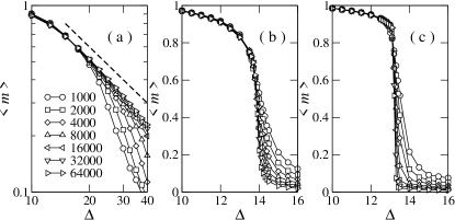
Figure 2: $\langle m\rangle$ versus $\Delta$ with the magnetic field distribution $p(h)=p_{+}(h/\Delta)/\Delta$ and $\gamma=2.5$ (a), 4.0 (b), and 6.0 (c). The dashed line in (a) has a slope $-1$.

At $\gamma=2.5$, the ferromagnetic order with nonzero $m$ persists at high values of $\Delta$. Moreover, the log-log plot in Fig. 2(a) suggests that the magnetization decreases algebraically. This behavior is consistent with the analytic result $m\sim\Delta^{-(\gamma-2)/(3-\gamma)}$ in Eq. (21). According to it, the decay exponent should be $-1$ at $\gamma=2.5$. There is a little discrepancy in the decay exponent. We attribute the apparent discrepancy to a finite-size effect since the decay exponent approaches the analytic result as $N$ increases. However, we cannot exclude a possibility that it could be due to the negative degree correlation at $\gamma=2.5$.

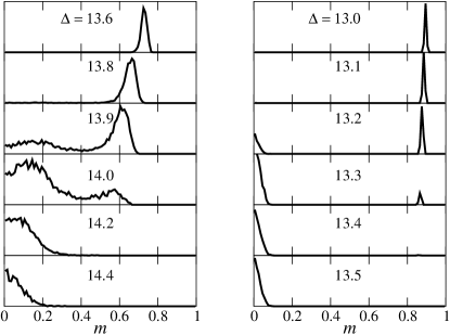
Figure 3: The histogram on an arbitrary scale of the magnetization at several values of $\Delta$ near the transition on the SF networks of $N=64000$ nodes with $\gamma=4.0$ (left column) and 6.0 (right column).

Figures 2(b) and 2(c) show that the order parameter vanishes abruptly at a certain threshold of $\Delta$, which is a characteristic of a first-order phase transition. In order to prove the first-order nature we study the order parameter histogram $H(m)$ near the threshold. Numerically the histogram is measured by the fraction of samples whose order parameter value lies between $m$ and $m+\delta m$, which is equal to $H(m)\delta m$. In Fig. 3, we present the histogram $H(m)$ obtained numerically on the SF networks of $N=64000$ nodes with $\delta m=0.01$. At small values of $\Delta$ the histogram is peaked at a nonzero value of $m$, while it is peaked at $m=0$ at high values of $\Delta$. In the intermediate values of $\Delta$, there appear two peaks in the histogram, which indicates the phase coexistence. The two-peak structure near the threshold confirms the first-order transition nature.

III.2 Numerical result with $p(h)=p_{-}(h/\Delta)/\Delta$

We present the numerical data obtained with the random field distribution $p(h)=p_{-}(h/\Delta)/\Delta$ in Fig. 4. At $\gamma=2.5$ [Fig. 4(a)], the order parameter remains finite and decreases algebraically as $\Delta$, which is consistent with Eq. (21). At $\gamma=4.0$ and $6.0$ [Figs. 4(b) and 4(c)], the order parameter shows a threshold behavior. Unlike the case with $p(h)=p_{+}(h/\Delta)/\Delta$, the order parameter approaches zero smoothly as $\Delta$ increases. It indicates that the transition could be a continuous transition.

In order to examine the transition nature, we measure the Binder parameter BindersCumulant

$$U=1-\frac{\langle m^{4}\rangle}{3\langle m^{2}\rangle^{2}}.$$ (24)

The Binder parameter is supposed to take a nontrivial value at a critical point with scale invariance. It takes a trivial value $2/3$ and $0$ in an ordered phase and in a disordered phase, respectively, in the $N\to\infty$ limit. A critical point will manifest itself as a crossing point in the plot of $U$ versus $\Delta$ at different system sizes $N$.

Figure 4: $\langle m\rangle$ versus $\Delta$ with $p(h)=p_{-}(h/\Delta)/\Delta$ and $\gamma=2.5$ (a), 4.0 (b), and 6.0 (c). The dashed line in (a) has a slope $-1$.

Figure 5: $U$ versus $\Delta$ for various system sizes with the degree exponent (a) $\gamma=2.5$, (b) $\gamma=4$, and (c) $\gamma=6$.

Figure 5 shows the Binder parameter for the three cases, each of which corresponds to $2<\gamma<3$, $3<\gamma<5$, and $\gamma>5$. In Fig. 5(a), there is no crossing point and the value $U=2/3$, corresponding to the ordered state, persists as the system size grows. This behavior clearly shows that the system is always magnetized in the thermodynamic limit. Figures 5(b) and 5(c) show that there appear the crossing points at $\Delta_{c}\simeq$ $38.0$ for $\gamma=4.0$ and $\Delta_{c}\simeq 31.5$ for $\gamma=6$ where the Binder parameter is scale invariant and the system is critical. It indicates that the transition is a continuous transition.

Since the phase transition is a continuous one, we expect that the order parameter satisfies the critical finite-size-scaling form BindersCumulant

$$\langle m\rangle=N^{-\beta/\nu^{\prime}}F((\Delta_{c}-\Delta)^{\nu^{\prime}}N),$$ (25)

where $\beta$ is the order parameter exponent and $\nu^{\prime}$ is the finite-size-scaling exponent. The scaling function $F(x)$ has the limiting behavior that $F(x\to 0)\sim\mbox{const}$ and $F(x\to\infty)\sim x^{\beta/\nu^{\prime}}$ so that

$$\langle m\rangle\sim(\Delta_{c}-\Delta)^{\beta}$$ (26)

for $N\gg(\Delta_{c}-\Delta)^{-\nu^{\prime}}$ and

$$\langle m\rangle\sim N^{-\beta/\nu^{\prime}}$$ (27)

for $N\ll(\Delta_{c}-\Delta)^{-\nu^{\prime}}$.

The finite-size-scaling form is used to obtain the critical exponents $\beta$ and $\nu^{\prime}$. In Fig. 6, we present the scaling plot for the order parameter according to Eq. (25) with the exponent values that give the best data collapse. We estimate that $\beta=0.75$ and $\nu^{\prime}=3.47$ for $\gamma=4.0$ and $\beta=0.45$ and $\nu^{\prime}=2.81$ for $\gamma=6.0$.

Figure 6: Scaling plot of $\langle m\rangle N^{\beta/\nu^{\prime}}$ versus $|\Delta_{c}-\Delta|^{\nu^{\prime}}N$ for $\gamma=4.0$ in (a) and $\gamma=6.0$ in (b).

Repeating the same analysis, we obtained the values of $\beta$ at several values of $\gamma>3$. The numerical results are compared with the analytic mean-field results [see Eqs. (18) and (15)] in Fig. 7. For $\gamma>5$, the critical exponent $\beta$ is indeed $1/2$ from the simulation result. One finds that the values of $\beta$ for $3<\gamma<5$ deviate slightly from the mean-field prediction. Although we suspect that this may be due to the singular dependence of $\beta=1/(\gamma-3)$ near $\gamma=3$, we cannot exclude a possibility that it may be due to a limitation of the our mean-field approximation.

Figure 7: The critical exponent $\beta$ as a function of the degree exponent $\gamma$. The solid line corresponds to the mean-field result $\beta=1/(\gamma-3)$ for $3<\gamma<5$ and $\beta=1/2$ for $\gamma>5$. The numerical simulation is based on the finite-size-scaling method.

IV discussion and conclusions

The main result of our work is that the RFIM on scale-free networks is always magnetized for $2<\gamma<3$ and it has a disorder-driven phase transition for $\gamma>3$ whose nature depends on the shape of the random field distribution $p(h)=p_{0}(h/\Delta)/\Delta$. As for the nature of the transition, similar results have been known in regular lattices in high-dimensional Euclidean space Schneider1977 ; Aharony1978 ; Swift1997 : the disorder-driven zero-temperature phase transition is first order or continuous for a convex ($p^{\prime\prime}(0)>0$) or concave ($p^{\prime\prime}(0)<0$) random field distribution, respectively. Our result shows that the same criterion is valid for SF networks with $\gamma>5$. For $3<\gamma<5$, the criterion is replaced by positivity or negativity of the quantity $D$ defined in Eq. (17). Roughly speaking, the distributions $p(h)$ highly peaked at $h=0$ give rise to the continuous transition, while distributions highly peaked at nonzero $h=\pm h_{0}$ give rise to the first-order transition. One may have a distribution with $p^{\prime\prime}_{0}(0)>0$ but with $D<0$. For example, $p_{0}(-1<x<1)=3[a+(1-a)x^{2}]/[2(1+2a)]$ with $a=3/4$ is such a function. We checked numerically that it indeed leads to the continuous phase transition at $\gamma=4$.

In summary, we have investigated the RFIM on scale-free networks with inhomogeneous connections. The network topology, especially the degree exponent $\gamma$, is shown to affect the phase transition and the critical exponent. The shape of the random field distribution is also responsible for the nature of the phase transition.

- (1) R. Albert and A.-L. Barabási, Rev. Mod. Phys. 74, 47 (2002).
- (2) M. E. J. Newman, SIAM Rev. 45, 167 (2003).
- (3) S. N. Dorogovtsev and J. F. F. Mendes, Adv. Phys. 51, 1079 (2002); Evolution of Networks: From Biological Nets to the Internet and WWW (Oxford University Press, Oxford, 2003).
- (4) A. Pekalski, Phys. Rev. E 64 057104 (2001).
- (5) H. Hong, B. J. Kim, and M. Y. Choi, Phys. Rev. E 66 018101 (2002).
- (6) B. J. Kim, H. Hong, P. Holme, G. S. Jeon, P. Minnhagen, and M. Y. Choi, Phys. Rev. E 64, 056135 (2001).
- (7) J. Viana Lopes, Y. G. Pogorelov, J. M. B. Lopes dos Santos, and R. Toral, Phys. Rev. E 70, 026112 (2004).
- (8) D. Jeong, M. Y. Choi, and H. Park, Phys. Rev. E 71, 036103 (2005).
- (9) V. Sood and S. Redner, Phys. Rev. Lett. 94, 178701 (2005).
- (10) A. V. Goltsev, S. N. Dorogovtsev, and J. F. F. Mendes, Phys. Rev. E 67, 026123 (2003).
- (11) S. N. Dorogovtsev, A. V. Goltsev, and J. F. F. Mendes, Eur. Phys. J. B 38, 177 (2004).
- (12) F. Iglói and L. Turban, Phys. Rev. E 66, 036140 (2002).
- (13) Q. Michard and J.-P. Bouchaud, Eur. Phys. J. B 47, 151 (2005).
- (14) S.-W. Son, H. Jeong, and J. D. Noh, Eur. Phys. J. B 50, 431 (2006).
- (15) R. Pastor-Satorras and A. Vespignani, Phys. Rev. Lett. 86, 3200 (2001).
- (16) M. Catanzaro, M. Boguñá, and R. Pastor-Satorras, Phys. Rev. E 71, 056104 (2005).
- (17) D.-H. Kim, G. J. Rodgers, B. Kahng, and D. Kim, Phys. Rev. E 71, 056115 (2005).
- (18) J. M. Mooij and H. J. Kappen, e-print cond-mat/0408378.
- (19) T. Schneider and E. Pytte, Phys. Rev. B 15, 1519 (1977).
- (20) A. Aharony, Phys. Rev. B 18, 3318 (1978).
- (21) J. Villain, Phys. Rev. Lett. 52, 1543 (1984).
- (22) R. Bruinsma and G. Aeppli, Phys. Rev. Lett. 52, 1547 (1984).
- (23) J. Z. Imbrie, Phys. Rev. Lett. 53, 1747 (1984).
- (24) M. E. J. Newman and G. T. Barkema, Phys. Rev. E 53, 393 (1996).
- (25) A. A. Middleton and D. S. Fisher, Phys. Rev. B 65, 134411 (2002).
- (26) M. R. Swift, A. J. Bray, A. Maritan, M. Cieplak, and J. R. Banavar, Europhys. Lett. 38, 273 (1997).
- (27) J.-C. Anglès d’Auriac and N. Sourlas, Europhys. Lett. 39, 473 (1997).
- (28) M. Mézard, G. Parisi, and M. A. Virasoro, Spin Glass Theory and Beyond (World Scientific, Singapore, 1987).
- (29) M. E. J. Newman, Phys. Rev. Lett. 89, 208701 (2002).
- (30) Generalization to an arbitrary is straightforward.
- (31) M. E. J. Newman, S. H. Strogatz, and D. J. Watts, Phys. Rev. E 64, 026118 (2001).
- (32) R. Cohen, K. Erez, D. ben-Avraham, and S. Havlin, Phys. Rev. Lett. 85, 4626 (2000).
- (33) K.-I. Goh, B. Kahng, and D. Kim, Phys. Rev. Lett. 87, 278701 (2001).
- (34) J.-S. Lee, K.-I. Goh, B. Kahng, and D. Kim, Eur. Phys. J. B 49, 231 (2006).
- (35) M. Alava, P. M. Duxbury, C. Moukarzel, and H. Rieger, in Phase Transitions and Critical Phenomena edited by C. Domb and J. L. Lebowitz (Academic, Cambridge, England, 2000) Vol. 18, pp. 141-317; A. Hartmann and H. Rieger, Optimization Algorithms in Physics (Wiley VCH, Berlin, 2002).
- (36) K. Binder and D. W. Heerman, Monte Carlo Simulation in Statistical Physics, 2nd ed. (Springer-Verlag, Berlin, 1992).