Scalable superconducting qubit circuits using dressed states

Abstract

We study a coupling/decoupling method between a superconducting qubit and a data bus that uses a controllable time-dependent electromagnetic field (TDEF). As in recent experiments, the data bus can be either an LC circuit or a cavity field. When the qubit and the data bus are initially fabricated, their detuning should be made far larger than their coupling constant, so these can be treated as two independent subsystems. However, if a TDEF is applied to the qubit, then a “dressed qubit” (i.e., qubit plus the electromagnetic field) can be formed. By choosing appropriate parameters for the TDEF, the dressed qubit can be coupled to the data bus and, thus, the qubit and the data bus can exchange information with the assistance of the TDEF. This mechanism allows the scalability of the circuit to many qubits. With the help of the TDEF, any two qubits can be selectively coupled to (and decoupled from) a common data bus. Therefore, quantum information can be transferred from one qubit to another.

I Introduction

Superconducting qubits phy are promising candidates for quantum information processing and their macroscopic quantum coherence has been experimentally demonstrated. Single superconducting qubit experiments also motivate both theorists and experimentalists to explore the possibility for scaling up to many qubits.

Two-qubit experiments have been performed in superconducting charge pashkin , flux izmalkov ; majer ; plourde1 , and phase qubit berkley ; xu ; mcdermott circuits. One of the basic requirements for scalability to many qubits is to selectively couple any pair of qubits. However, these experimental circuits pashkin ; izmalkov ; majer ; plourde1 ; berkley ; xu ; mcdermott are difficult to scale up to many qubits, due to the existence of the always-on interaction. Theoretical proposals (e.g., Refs. makhlin ; you2 ; jqprl ; you1 ; blais ; liuyx ; zagoskin ; migliore ; blais1 ; cleland ) have been put forward to selectively couple any pair of qubits through a common data bus (DB). Some proposals (e.g., Refs. makhlin ; you2 ; jqprl ) only involve virtual excitations of the DB modes, while in others (e.g., Refs. you1 ; blais ; liuyx ; zagoskin ; migliore ; blais1 ; cleland ), the DB modes need to be excited. In these proposals (e.g., Refs.  makhlin ; you2 ; jqprl ), the controllable coupling is implemented by the fast change of the external magnetic flux, which is a challenge for current experiments. The switchable coupling between any pair of qubits can also be implemented by adding additional subcircuits (e.g., in Refs. averin ; plourde ). These additional elements increase the complexity of the circuits and also might add additional uncontrollable noise.

Recently, two theoretical approaches rigetti ; liu1 using time-dependent electromagnetic fields have been proposed to control the coupling between two qubits. Both proposals require that: (i) the detuning between the two qubits is far larger than their coupling constant; and thus the ratio between the coupling constant and the detuning is negligibly small. In this case, the two qubits can be considered as two independent subsystems mcdermott . (ii) To couple two qubits, the appropriate time-dependent electromagnetic fields (TDEFs) or variable-frequency electromagnetic fields must be applied to the qubits, to achieve coupling/decoupling.

However, there are significant differences between these two approaches rigetti ; liu1 . Some are described below.

(i) In the proposal rigetti , two dressed qubits are formed by the two decoupled qubits and their corresponding TDEFs. If the parameters of the applied TDEFs are appropriately chosen so that the transition frequencies of the two dressed qubits are the same, then the resonant coupling of the two dressed qubits is realized, and the information between two decoupled qubits can be exchanged with the help of the TDEFs. However, for another proposal liu1 , one TDEF is enough to achieve the goal of exchanging information between two decoupled qubits. This works because there is a nonlinear coupling liu1 between the applied TDEF and the two decoupled qubits. If the frequency of the applied TDEF is equal to either the detuning (i.e., the difference) or the sum of the frequencies of the two qubits, then these two qubits are coupled to each other and information between these two qubits can be exchanged.

(ii) For the case in Ref. rigetti , when two qubits are coupled to each other, the original basis states of each qubit are mixed by the TDEF, but the frequencies of the qubits remain unchanged. However, for the proposal in Ref. liu1 , both basis states and transition frequencies of the two qubits remain unchanged during the coupling/decoupling processes.

The approach in Ref. liu1 can be used to scale up to many qubits by virtue of a common DB liu2 , in analogy with quantum computing with trapped ions cirac ; sasura ; wei1 , and in contrast with the circuit QED approach you1 ; blais ; liuyx ; zagoskin ; migliore ; wallraff ; circuitQED . The essential differences between the “trapped ion” proposal for superconducting qubits liu2 and the circuit QED you1 ; blais ; liuyx ; zagoskin ; migliore ; wallraff ; circuitQED approach are the following.

(a) When a TDEF is applied to the selected qubit, there are nonlinear coupling terms liu2 between that qubit, the DB and the TDEF, but these terms do not appear in the circuit QED proposal you1 ; blais ; liuyx ; zagoskin ; migliore ; wallraff ; circuitQED . This significant difference provides different coupling mechanisms for these two proposals.

(b) In Ref. liu2 , the frequencies of the qubit and the data bus always remain unchanged during operations, including coupling and decoupling. But these frequencies are changed in the coupling and decoupling stages for the circuit QED (e.g., in Refs. wallraff ; circuitQED ).

(c) The qubit-DB coupling is realized in the proposal liu2 by applying a TDEF so that the frequency of the applied TDEF is equal to the detuning or sum of the frequencies of the qubit and the data bus; but this qubit-DB coupling is realized by changing the qubit frequency, so that it becomes equal to the DB frequency in the circuit QED.

(d) Without an applied TDEF used for the “trapped ion” proposal liu2 , the qubit and the DB are decoupled liu2 . In contrast, in the circuit QED (e.g., in Refs. wallraff ; circuitQED ), the decoupling is realized by changing the qubit frequency such that the qubit and the DB have a very large detuning.

From (b), (c), and (d), it is clear that, in circuit QED, the Hilbert spaces of the qubit and the data bus are always changed during the coupling/decoupling stage. But, in the “trapped ion” approach liu2 , the Hilbert spaces of the qubit and the data bus remain unchanged during the coupling/decoupling processes .

Also, after our papers in Ref. liu1 and Ref. liu2 were submitted, other groups bertet ; nec followed our proposal of using the nonlinear coupling between the qubits and the TDEF to control the couplings among qubits. Our approach liu1 ; liu2 works when the frequency of the TDEF is equal to either the detuning or the sum of the frequencies of the two qubits (or the qubit and the data bus), then the coupling between the two qubits is realized, otherwise, these two qubits are decoupled liu1 ; liu2 .

Motivated by the “dressed qubits” proposal rigetti , in this paper, we study how to scale up to many qubits using a common DB and TDEFs. Our paper is organized as follows. In Sec. II, we describe the Hamiltonian of a superconducting flux qubit coupled to an LC circuit–DB. We explain the decoupling mechanism using dressed qubits, and then further explain how the qubit can be coupled to the DB with the help of the TDEF. In Sec. III, the dynamical evolution of the qubit and the data bus is analyzed. In Sec. IV, the scalability of our proposed circuit is discussed. We analyze the implementation of single-qubit and two-qubit gates with the assistance of the TDEFs. In Sec. V, we discuss how to generate entangled states. In Sec. VI, we use experimentally accessible parameters to discuss the feasibility of our proposal.

II Dressed states and coupling mechanism

II.1 Model

For simplicity, we first consider a DB interacting with a singe qubit. Generally, the DB can represent either a single-mode light field you1 ; blais ; liuyx ; zagoskin ; migliore , an LC oscillator (e.g., Refs. liu2 ; plastina ; ntt ), a large junction buisson ; wei ; wang ; zhou , or other similar elements which can be modeled by harmonic oscillators. The qubit can be either an atom, a quantum dot, or a superconducting quantum circuit with a Josephson junction—working either in the charge, phase, or flux regime.

Without loss of generality, we now study a quantum circuit, shown in Fig. 1, constructed by a superconducting flux qubit and an LC circuit acting as a data bus. The interaction between a single superconducting flux qubit and an LC circuit has been experimentally realized ntt . The flux qubit consists of three junctions with one junction smaller by a factor $0.5<\alpha<1$ than the other two, identical, junctions. The LC circuit interacts with the qubit through their mutual inductance $M$. Then, the total Hamiltonian of the qubit and the data bus can be written liu2 ; ntt as

$$H_{0}=\hbar\omega a^{\dagger}a+\frac{\hbar}{2}\omega_{q}\,\sigma_{z}+\hbar\left(\chi\sigma_{+}a+{\rm h.c.}\right),$$ (1)

in the rotating wave approximation. Here, the qubit operators are defined by $\sigma_{z}=|e\rangle\langle e|-|g\rangle\langle g|$, $\sigma_{+}=|e\rangle\langle g|$, and $\sigma_{-}=|g\rangle\langle e|$; using its ground $|g\rangle$ and first excited $|e\rangle$ states. The qubit frequency $\omega_{q}$ in Eq. (1) can be expressed orlando ; cyclic as

$$\hbar\omega_{q}=2\sqrt{I^{2}\left(\Phi_{\rm e}-\frac{\Phi_{0}}{2}\right)^{2}+T_{RL}^{2}}$$

with the bias flux $\Phi_{\rm e}$ and the qubit alec loop-current $I$. The parameter $T_{RL}$ denotes the tunnel coupling between the two potential wells of the qubit orlando . The ladder operators $a$ and $a^{\dagger}$ of the LC circuit are defined by

$$a = \sqrt{\frac{C\omega}{\hbar}}\,\varphi+i\,\sqrt{\frac{1}{\hbar C\omega}}\,Q,$$ (2a)

$$a^{\dagger} = \sqrt{\frac{C\omega}{\hbar}}\,\varphi-i\,\sqrt{\frac{1}{\hbar C\omega}}\,Q,$$ (2b)

for the magnetic flux $\varphi$ through the LC circuit and the charge $Q$ stored on the capacitor $C$ of the LC circuit with the self-inductance $L$. The frequency of the LC circuit is $\omega=1/\sqrt{LC}$. The magnetic flux $\varphi$ and the charge $Q$ satisfy the commutation relation $[Q,\,\varphi]=i\hbar$. The coupling constant $\chi$ between the qubit and the LC circuit can be written as

$$\chi=M\sqrt{\frac{\hbar\omega}{2L}}\,\langle e|I|g\rangle.$$

Figure 1: (Color online) A three-junction flux qubit is coupled to an LC circuit by their mutual inductance $M$. The dc bias magnetic flux through the qubit is $\Phi_{e}$. A time-dependent magnetic field $\Phi_{e}(t)$ can be applied to the qubit, so the qubit can be coupled to the LC circuit. Further details are explained in the text.

II.2 Decoupling mechanism between qubit and LC circuit

Below, we assume that the detuning $\omega_{q}-\omega$ between the LC circuit and the qubit is larger than their coupling constant $\chi$, i.e., without loss of generality, $\omega_{q}-\omega\gg|\chi|$. In this large-detuning condition, instead of the Hamiltonian $H_{0}$ in Eq. (1), the dynamical evolution (of the qubit and the LC circuit) is governed by the effective Hamiltonian sun

$$H_{0}^{E}=\hbar\omega_{-}\,a^{\dagger}a+\frac{\hbar}{2}\omega_{q}\sigma_{z}+\hbar\frac{|\chi|^{2}}{\omega_{q}-\omega}(1+2a^{\dagger}a)|e\rangle\langle e|,$$ (3)

with $\omega_{+}=\omega-|\chi|^{2}/(\omega_{q}-\omega)$. Equation (3) shows that the interaction between the LC circuit and the qubit results in a dispersive shift of the cavity transition or a Stark/Lamb shift of the qubit frequency $\omega_{q}$. In this large detuning condition, the qubit states cannot be flipped by virtue of the interaction with the LC circuit.

Obviously, if the ratio $|\chi|/(\omega_{q}-\omega)$ tends to zero, then the third term in Eq. (3) also tends to zero and $\omega_{-}\approx\omega$. In this limit, the coupling between the qubit and the data bus can be neglected, that is,

$$H_{0}^{E}\,\approx\,\hbar\omega a^{\dagger}a+\frac{\hbar}{2}\omega_{q}\sigma_{z}.$$

The qubit and the LC circuit can be considered as two independent subsystems, which can be separately controlled or manipulated. Below, we assume that the LC circuit and the qubit satisfy the large-detuning condition, e.g., $|\chi|/(\omega_{q}-\omega)\sim 0$, when they are initially fabricated, so they are approximately decoupled.

II.3 Dressed states

We now apply a TDEF to the qubit such that the dressed qubit can be formed by the applied TDEF and the qubit. Let us assume that the qubit, driven now by the TDEF, works at the optimal point cyclic . In this case, the total Hamiltonian $H$ of the LC circuit and the qubit driven by a TDEF can be written ntt as

$$H = H_{0}+\hbar\left(\lambda e^{-i\omega_{c}t}\sigma_{+}+{\rm H.c.}\right),$$ (4)

in the rotating wave approximation. Here $\omega_{c}$ is the frequency of the TDEF applied to the qubit. $\lambda$ is the Rabi frequency of the qubit associated with the TDEF. We note that now the nonlinear coupling strength liu2 between the qubit, LC circuit and the TDEF is zero since the qubit works at the optimal point.

Since a unitary transformation does not change the eigenvalues of the system, in the rotating reference frame through a unitary transformation $U_{R}=\exp(-i\omega_{c}\,\sigma_{z}t/2)$, the Hamiltonian in Eq. (4) is equivalently transferred to an effective Hamiltonian

$$H_{e}=U^{\dagger}_{R}H\,U_{R}-i\hbar U^{\dagger}_{R}\left(\frac{dU_{R}}{dt}\right).$$ (5)

Hereafter, unless specified otherwise we work in the rotating reference frame. We can divide the Hamiltonian $H_{e}$ in two parts, i.e., $H_{e}=H^{(1)}_{e}+H^{(2)}_{e}$ with

$$H_{e}^{(1)} = \hbar\omega a^{\dagger}a+\hbar\left(\chi a\,\sigma_{+}\,e^{i\omega_{c}t}+{\rm H.c.}\right),$$ (6a)

$$H_{e}^{(2)} = \frac{\hbar}{2}\,\Delta\,\sigma_{z}+\hbar\left(\lambda\,\sigma_{+}+{\rm H.c.}\right),$$ (6b)

where $\Delta=\omega_{q}-\omega_{c}$. The Hamiltonian $H_{e}^{(2)}$ can be diagonalized and rewritten as

$$H_{e}^{(2)}=\frac{\hbar}{2}\Omega\rho_{z}$$ (7)

with the transition frequency

$$\Omega\,=\,\sqrt{(\omega_{q}-\omega_{c})^{2}+4|\lambda|^{2}}.$$

Here, $\rho_{z}$ is given by $\rho_{z}=|E\rangle\langle E|-|G\rangle\langle G|$ in the new basis states

$$|E\rangle = \cos\frac{\eta}{2}|e\rangle+e^{i\phi}\sin\frac{\eta}{2}|g\rangle,$$ (8a)

$$|G\rangle = -\sin\frac{\eta}{2}|e\rangle+e^{i\phi}\cos\frac{\eta}{2}|g\rangle,$$ (8b)

with $\eta=\tan^{-1}(2|\lambda|/\Delta)$. The eigenvalues $E$ and $G$, corresponding to the eigenstates $|E\rangle$ and $|G\rangle$, are denoted by

$$E\;=\;-G\;=\;\frac{\hbar}{2}\sqrt{\Delta^{2}+4|\lambda|^{2}}.$$ (9)

The phase $\phi$ is related to the Rabi frequency $\lambda$ ($\lambda=|\lambda|e^{-i\phi}$), and the phase $\phi$ can be controlled by the applied TDEF. In Fig. 2, the dependence of the eigenvalues $E$ and $G$ on the detuning $\Delta=\omega_{q}-\omega_{c}$ and the amplitude of the Rabi frequency $|\lambda|$ has been plotted. The gap between these two surfaces corresponds to the frequency $\Omega/2\pi$ of the dressed qubit. It clearly shows that $\Omega$ can be changed by $\omega_{c}$ when $|\lambda|$ and $\omega_{q}$ are given, and also changed by $|\lambda|$ when $\omega_{c}$ and $\omega_{q}$ are given. The larger of $|\lambda|$ and $\Delta$ corresponds to the larger transition frequency $\Omega$ of the dressed qubit.

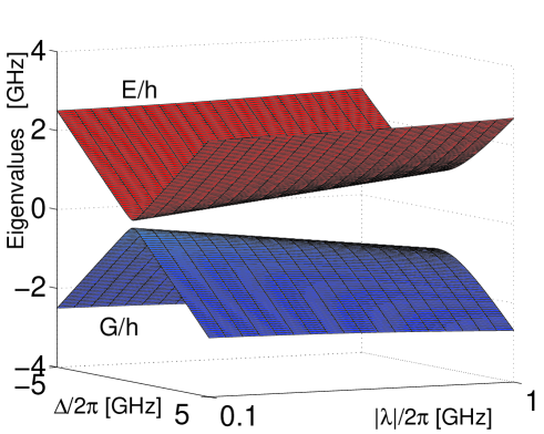
Figure 2: (Color online) The dependence of the eigenvalues $E$ and $G$ of Eq. (9) on the detuning frequency $\Delta/2\pi=(\omega_{q}-\omega_{c})/2\pi$ and the amplitude of the Rabi frequency $|\lambda|/2\pi$. Here, the eigenvalues have been rescaled as frequencies, i.e., $E/h$ and $G/h$. The gap between these two surfaces corresponds to the frequency $\Omega/2\pi$ of the dressed qubit.

In fact, the states $|E\rangle$ and $|G\rangle$ could be interpreted as the dressed states of the qubit and the TDEF cohen . Usually, the applied TDEF is considered as in a coherent state cohen , e.g., $|\alpha\exp(-i\omega_{c}t)\rangle$. If the creation and annihilation operators of the TDEF are represented by $b^{\dagger}$ and $b$, then the state $|\alpha\exp(-i\omega_{c}t)\rangle$ is an eigenstate of the operator $b$ with the eigenvalue $\alpha\exp(-i\omega_{c}t)$. The average photon number $\overline{N}$ of the TDEF in this coherent state is $\overline{N}=|\alpha|^{2}$, and the width $\delta\overline{N}$ of the number distribution of photons for the applied TDEF is $\delta\overline{N}=|\alpha|$.

In the limit $\overline{N}\gg\delta\overline{N}\gg 1$, the photon number, absorbed and emitted by the qubit, is negligibly small, and the qubit is always assumed to be subjected to the same intensity $|\alpha|^{2}$ of the applied TDEF during the operation. Therefore, the TDEF operators $b$ and $b^{\dagger}$ can be replaced by the classical number $\alpha\exp(-i\omega_{c}t)$ and its complex conjugate. The relation between $\alpha$ and the Rabi frequency $\lambda$ of the qubit associated with the applied TDEF is $|\lambda|\propto|\alpha|$. And also the coherent state $|\alpha\exp(-i\omega_{c}t)\rangle$, representing the TDEF, and the qubit state can always be factorized at any time.

In the rotating reference frame, the coherent state of the TDEF is always $|\alpha\rangle$, and the dressed qubit-TDEF states $|E\rangle_{D}$ and $|G\rangle_{D}$ can be understood as the product state of $|E\rangle$ (or $|G\rangle$) and $|\alpha\rangle$, that is,

$$|E\rangle_{D} = \left(e^{i\phi}\sin\frac{\eta}{2}|g\rangle+\cos\frac{\eta}{2}|e\rangle\right)|\alpha\rangle=|E\rangle|\alpha\rangle,$$ (10a)

$$|G\rangle_{D} = \left(e^{i\phi}\cos\frac{\eta}{2}|g\rangle-\sin\frac{\eta}{2}|e\rangle\right)|\alpha\rangle=|G\rangle|\alpha\rangle.$$ (10b)

Therefore, the photon state $|\alpha\rangle$ of the TDEF is usually omitted when the dressed states are constructed by the qubit and the TDEF, e.g., in Eq. (8). Hereafter, in contrast to the dressed states $|G\rangle$ and $|E\rangle$, $|g\rangle$ and $|e\rangle$ are called “bare” or undressed qubit states.

If we assume $\omega>\omega_{c}$, then in the dressed-state basis of Eq. (8), the effective Hamiltonian $H_{e}$ can be rewritten as

$$H_{e}=\hbar\,\omega a^{\dagger}a+\frac{\hbar}{2}\Omega\rho_{z}+\hbar(\kappa\,\rho_{-}a^{\dagger}e^{-i\omega_{c}t}+{\rm H.c.})$$ (11)

with the coupling constant

$$\kappa=\chi\cos^{2}(\eta/2)$$

between the dressed qubit and the LC circuit–DB. The ladder operator $\rho_{-}$ is defined as $\rho_{-}=|G\rangle\langle E|$. Here, the terms $(\chi/2)\,\sin(\eta)\,\rho_{z}\,a\,e^{i\omega_{c}t}$, $\sin^{2}(\eta/2)\,\rho_{-}\,a\,e^{-i\omega_{c}t}$, and their complex conjugates have been neglected because of the following reason: there is no way to conserve energies in these terms, and then they can be neglected by using the usual rotating-wave approximation.

II.4 Coupling mechanism between qubit and LC circuit

To better understand the coupling mechanism, we can rewrite the Hamiltonian of Eq. (11), in the interaction picture, as

$$H_{e,{\rm int}}=\hbar\kappa\,\rho_{-}a^{\dagger}e^{i[(\omega-\omega_{c})-\Omega]t}+{\rm H.c.}\,.$$ (12)

Obviously, the condition

$$\Omega=\omega-\omega_{c}$$ (13)

is satisfied when the fast oscillating factor $e^{i[(\omega-\omega_{c})-\Omega]t}$ and its complex conjugate are always one. In this case, the Hamiltonian (12) becomes

$$H_{e,{\rm int}}=\hbar\kappa\,\rho_{-}\,a^{\dagger}+{\rm H.c.}\,.$$ (14)

The resonant condition in Eq. (13) can always be satisfied by choosing the appropriate frequency $\omega_{c}$ of the TDEF and the Rabi frequency $\lambda$. Therefore, the dressed qubit can resonantly interact with the LC circuit, and then the information can be exchanged between the qubit and the LC circuit with the help of the TDEF.

II.5 An example of coupling between a qubit and an LC circuit

We now numerically demonstrate the coupling and decoupling mechanism. For example, let us consider a qubit with frequency $\omega_{q}/2\pi=2$ GHz which works at the optimal point; the frequency of the LC circuit is $\omega/2\pi\sim 4$ GHz; and the coupling constant $|\chi|$ between the LC circuit and the qubit is $200$ MHz. In this case, the ratio $|\chi|/(\omega-\omega_{q})=0.1$, and the Stark/Lamb shift for the qubit frequency is about $20$ MHz, which is much smaller than the qubit frequency of $2$ GHz. In this case, the interaction between the qubit and the LC circuit only results in an ac Stark/Lamb shift, but cannot make qubit states flip.

If we apply a TDEF such that the frequency $\Omega$ of the dressed qubit satisfies the condition in Eq. (13), then the qubit states can be flipped by the interaction with the LC circuit with the help of the TDEF. In Fig. 3, the transition frequency of the dressed qubit

$$\Omega=\sqrt{(\omega_{q}-\omega_{c})^{2}+4|\lambda|^{2}}$$

and the frequency difference $(\omega-\omega_{c})/2\pi$ are plotted as a function of the frequency $\nu_{c}=\omega_{c}/2\pi$ of the TDEF for the above given frequencies of the qubit and the LC circuit when the Rabi frequency of the qubit associated with the TDEF $|\lambda|/2\pi=0.2$ GHz. Figure 3 shows that when the frequency of the TDEF is $\nu_{c}=\omega_{c}/2\pi\approx 2.96$ GHz, the condition $\Omega=\omega-\omega_{c}$ satisfied, and then the qubit is coupled to the LC circuit with the assistance of the TDEF. Threfore, the qubit state can be flipped by virtue of the interaction with the LC circuit with the help of the TDEF.

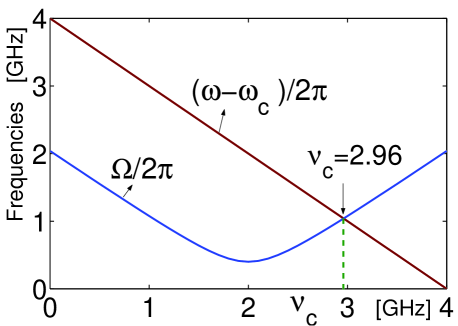
Figure 3: (Color online) The frequency $\Omega/2\pi$ of a dressed qubit (blue curve) and the frequency difference $(\omega-\omega_{c})/2\pi$ (dark red line); both versus the frequency $\nu_{c}=\omega_{c}/2\pi$ of the TDEF for the qubit frequency $\omega_{q}/2\pi=2$ GHz. The frequency of the LC circuit is $\omega/2\pi=4$ GHz; and the Rabi frequency of the qubit associated with the TDEF is $|\lambda|/2\pi=0.2$ GHz. The crossing point denotes the value of $\nu_{c}\approx 2.96$ GHz when the condition $\Omega=\omega-\omega_{c}$ is satisfied.

This could be compared with the switchable coupling circuits in Ref. liu2 , where the qubit basis is always kept in $\{|g\rangle,\,|e\rangle\}$ no matter if the qubit is coupled to or decoupled from the LC circuit. Here, the qubit basis states (e.g., $|g\rangle$ and $|e\rangle$) will be mixed as in Eq. (8) in the process of the TDEF-assisted qubit and LC circuit coupling.

III Dynamical evolution of a dressed qubit interacting with an LC circuit

III.1 Resonant Case

According to the above discussions, the information of the qubit can be transferred to the data bus with the assistance of an appropriate TDEF. For convenience, we observe the total system in another rotating reference frame $V_{R}=\exp(i\omega_{c}\,\rho_{z}\,t/2)$, then an effective Hamiltonian from Eq. (11) can be obtained as

$$H^{R}_{e}=\hbar\,\omega a^{\dagger}a+\frac{\hbar}{2}(\Omega+\omega_{c})\rho_{z}+\hbar(\kappa\,\rho_{-}a^{\dagger}+{\rm H.c.})\,.$$ (15)

Therefore, the condition of resonant interaction between the dressed qubit and the data bus is $\Omega=\omega-\omega_{c}$, as obtained in Eq. (13). Here we need to emphasize that the basis states have been changed to $\{|G\rangle,\,|E\rangle\}$ when the qubit is coupled to the LC circuit with the assistance of the TDEF, but the qubit basis states are $\{|g\rangle,\,|e\rangle\}$ when the qubit is decoupled from the LC cirucit.

According to the Hamiltonian in Eq. (15), if the LC circuit and the qubit are initially in the state $|0,G\rangle=|0\rangle\otimes|G\rangle$, or $|n+1,\,G\rangle=|n+1\rangle\otimes|G\rangle$, or $|n,\,E\rangle=|n\rangle\otimes|E\rangle$, then they can evolve to the following states

$$|0,\,G\rangle \rightarrow |0,\,G\rangle,$$ (16a)

$$|n,\,E\rangle \rightarrow A(t)\left[\cos(\nu t)|n,\,E\rangle\right.$$ (16b)

$$- \left.ie^{i\delta}\sin(\nu t)|n+1,\,G\rangle\right],$$

$$|n+1,\,G\rangle \rightarrow A(t)\left[\cos(\nu t)|n+1,\,G\rangle\right.$$ (16c)

$$- \left.ie^{-i\delta}\sin(\nu t)|n,\,E\rangle\right],$$

with $A(t)=\exp[-i(2n+1)\omega t/2]$, $\nu=|\kappa|\sqrt{n+1}$, and $\kappa=|\kappa|e^{i\delta}=|\chi\cos^{2}(\eta/2)|e^{i\delta}$. It is obvious that the phase $\delta$ is determined by the coupling constant $\chi$ between the qubit and the LC circuit. Here, we note that the state $|n,\,E\rangle$ (or $|m,\,G\rangle$) denotes that the LC circuit is in the number state $|n\rangle$ (or $|m\rangle$), but the qubit is in the dressed state $|E\rangle$ (or $|G\rangle$).

In the following discussions, we focus on the case where the LC circuit is initially in a state $|0\rangle$ or $|1\rangle$. According to Eq. (16), we can obtain the following transformations

$$|0,\,G\rangle \rightarrow |0,\,G\rangle,$$ (17a)

$$|0,\,E\rangle \rightarrow B(t)\left[\cos(|\kappa|t)|0,\,E\rangle\right.$$ (17b)

$$- \left.ie^{i\delta}\sin(|\kappa|t)|1,\,G\rangle\right],$$

$$|1,\,G\rangle \rightarrow B(t)\left[\cos(|\kappa|t)|1,\,G\rangle\right.$$ (17c)

$$- \left.ie^{-i\delta}\sin(|\kappa|t)|0,\,E\rangle\right],$$

with $B(t)=\exp[-i\omega t/2]$.

III.2 Nonresonant case

Above, we assumed that the detuning $|\omega_{q}-\omega|$ between the qubit and the LC circuit is far larger than their coupling $|\chi|$, i.e., $|\chi|/(\omega_{q}-\omega)\sim 0$, and thus the qubit and the LC circuit are independent. Here we consider another nonresonant case between the dressed qubit and the LC circuit in Eq. (15). We assume that the detuning $\Lambda$ between the dressed qubit and the LC circuit satisfies the condition $|\kappa|/\Lambda\ll 1$ with $\Lambda=\Omega+\omega_{c}-\omega$, but the ratio $|\kappa|/\Lambda$ does not tend to zero. In this case, the dynamical evolution of the dressed qubit and the LC circuit is governed by an effective Hamiltonian

$$H^{D}_{e}=\hbar\omega_{-}a^{\dagger}a+\frac{\hbar}{2}\Omega^{\prime}\rho_{z}+\hbar\frac{|\kappa|^{2}}{\Lambda}(1+2a^{\dagger}a)|E\rangle\langle E|.$$ (18)

with $\omega_{-}=\omega-(|\kappa|^{2}/\Lambda)$ and $\Omega^{\prime}=\Omega+\omega_{c}$. Because the ratio $|\kappa|/\Lambda$ is not negligibly small, the Stark/Lamb shift of the dressed qubit frequency or the dispersive shift of the frequency of the LC circuit should be taken into account.

If the LC circuit and the dressed qubit are initially in states $|0,G\rangle$, $|1,\,G\rangle$, $|0,\,E\rangle$, or $|1,\,E\rangle$, then they evolve as follows:

$$|0,G\rangle \Rightarrow \exp\left(i\frac{\Omega^{\prime}}{2}t\right)|0,G\rangle,$$ (19)

$$|1,\,G\rangle \Rightarrow \exp\left\{i\left(-\omega+\frac{|\kappa|^{2}}{\Lambda}+\frac{\Omega^{\prime}}{2}\right)t\right\}|1,\,G\rangle,$$ (20)

$$|0,\,E\rangle \Rightarrow \exp\left\{-i\left(\frac{\Omega^{\prime}}{2}+\frac{|\kappa|^{2}}{\Lambda}\right)t\right\}|0,\,E\rangle,$$ (21)

$$|1,\,E\rangle \Rightarrow \exp\left\{-i\left(\omega+\frac{2|\kappa|^{2}}{\Lambda}+\frac{\Omega^{\prime}}{2}\right)t\right\}|1,\,E\rangle.$$ (22)

IV Scalable circuit and Quantum Operations

IV.1 Scalable circuit

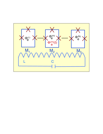
Figure 4: (Color online) The $N$ flux qubits are coupled to an LC circuit by the their mutual inductances $M_{m}$ ($m=1,\,\cdots,\,N$). The bias magnetic flux through the $m$th qubit is $\Phi_{e}^{(m)}$. A time-dependent electromagnetic field (TDEF) can be applied to any one of the qubits (e.g., $\Phi_{e}^{(m)}(t)$ through the $m$th qubit) such that the qubit can be coupled to the LC circuit with the help of the TDEF.

In the above, we show the basic mechanism of the coupling and decoupling between a superconducting flux qubit and the LC circuit. Therefore, a scalable quantum circuit, which is required for quantum information processing, can be constructed by $N$ flux qubits and an LC circuit acting as a data bus, shown in Fig. 4. The LC circuit interacts with $N$ qubits through their mutual inductances $M_{m}\,\,(m=1,\,2,\,\cdots,\,N)$. The distance between any two nearest qubits is assumed so large that their interaction through the mutual inductance can be negligibly small. Then, the total Hamiltonian of qubits and the data bus can be written liu2 as

$$H=\hbar\omega a^{\dagger}a+\frac{\hbar}{2}\sum_{m=1}^{N}\omega_{m}\sigma^{(m)}_{z}+\hbar\sum_{m=1}^{N}\left(\chi_{m}\sigma^{(m)}_{+}a+{\rm H.c.}\right)\,,$$ (23)

in the rotating wave approximation. Here, the $m$th qubit operators are defined as $\sigma^{(m)}_{z}=|e_{m}\rangle\langle e_{m}|-|g_{m}\rangle\langle g_{m}|$, $\sigma^{(m)}_{+}=|e_{m}\rangle\langle g_{m}|$, and $\sigma^{(m)}_{-}=|g_{m}\rangle\langle e_{m}|$ $(m=1,\,2,\,\cdots,\,N)$ using its ground $|g_{m}\rangle$ and the first excited $|e_{m}\rangle$ states. The $m$th qubit frequency $\omega_{m}$ in Eq. (23) can be expressed orlando as

$$\hbar\omega_{m}=2\sqrt{\left[I^{(m)}\left(\Phi^{(m)}_{\rm e}-\frac{\Phi_{0}}{2}\right)\right]^{2}+\left[T_{RL}^{(m)}\right]^{2}}$$

with the bias flux $\Phi^{(m)}_{\rm e}$ and its loop-current $I^{(m)}$ of the $m$th qubit alec ; liu2 . The parameter $T_{RL}^{(m)}$ denotes the tunnel coupling between two wells in the $m$th qubit orlando . The ladder operators $a$ and $a^{\dagger}$ of the LC circuit are defined as in Eq. (2). The coupling constant $\chi_{m}$ between the $m$th qubit and the LC circuit is

$$\chi_{m}=M_{m}\,\sqrt{\frac{\hbar\omega}{2L}}\,\langle e_{m}|I^{(m)}|g_{m}\rangle.$$

As in the above discussions, we assume that the detuning $\omega_{m}-\omega$ between the LC circuit and the $m$th ($m=1,\cdots,N$) qubit is far larger than their coupling constant $\chi_{m}$. That is, $\chi_{m}/(\omega_{m}-\omega)\sim 0$. Then, all $N$ qubits are decoupled from the LC circuit and each qubit can be independently manipulated by the TDEF. To couple a qubit to the LC circuit, an appropriate TDEF is needed to be applied such that the dressed qubit states can be formed, and then the dressed qubit can resonantly interact with the LC circuit.

For convenience, the parameters of any qubit are defined as follows. The frequency of the TDEF applied to the $m$th qubit is denoted by $\omega_{m,c}$. The detuning between the $m$th qubit frequency $\omega_{m}$ and $\omega_{m,c}$ is, $\Delta_{m}=\omega_{m}-\omega_{m,c}$; $\lambda_{m}$ is the Rabi frequency of the $m$th qubit associated with the TDEF. $|G_{m}\rangle$ and $|E_{m}\rangle$ are eigenstates of the $m$th qubit with the eigenvalues $G_{m}$ and $E_{m}$. The frequency of the $m$th dressed qubit is given by $\Omega_{m}$. The coupling constant between the $m$th qubit and the LC circuit is

$$\kappa_{m}=\chi_{m}\cos^{2}(\eta_{m}/2),$$

with $\eta_{m}={\rm tan}^{-1}(2|\lambda_{m}|/\Delta_{m})$.

We will now study how to implement the single- and two-qubit operations for the scalable circuit schematically shown in Fig. 4.

IV.2 Single-qubit Operations

The single-qubit operations of any qubit are easy to implement by applying a TDEF, which resonantly interacts with the selected qubit. For instance, if the frequency of the $m$th qubit is equal to the frequency $\omega_{m,c}$ of the applied TDEF, i.e., $\omega_{m,c}=\omega_{m}$, then the $m$th qubit rotation driven by the TDEF can be implemented by the single-qubit Hamiltonian $H_{m,s}$

$$H_{m,s}=\hbar|\lambda_{m}|\left(e^{-i\beta_{m}}\sigma^{(m)}_{+}+e^{i\beta_{m}}\sigma^{(m)}_{-}\right),$$ (24)

in the rotating reference frame through a unitary transformation $\exp(-i\omega_{m}\sigma_{z}t)$. Here, the phase $\beta_{m}$ is determined by the applied TDEF. The time evolution operator of the Hamiltonian in Eq. (24) can be wrrien as

$$U(\theta_{m},\beta_{m})=\exp\left[-i\frac{\theta_{m}}{2}\left(e^{-i\beta_{m}}\sigma^{(m)}_{+}+e^{i\beta_{m}}\sigma^{(m)}_{-}\right)\right],$$ (25)

with a duration $t$ and $\theta_{m}=2|\lambda_{m}|t$. Here, $U(\theta_{m},\beta_{m})$ is a general expression for a single-qubit operation. This unitary operator $U(\theta_{m},\beta_{m})$ can be rewritten as a matrix form

$$U(\theta_{m},\beta_{m})=\left[\begin{array}[]{cc}\cos(\theta_{m}/2)&-ie^{-i\beta_{m}}\sin(\theta_{m}/2)\\ -ie^{i\beta_{m}}\sin(\theta_{m}/2)&\cos(\theta_{m}/2)\end{array}\right].$$ (26)

Any single-qubit operation can be derived from Eq. (26). For instance, a rotation around the $x$ ($y$) axis can be implemented through Eq. (26) by setting the applied TDEF such that $\beta_{m}=0$ ($\beta_{m}=\pi/2$). It is worth pointing out that the operation in Eq. (26) is defined in the qubit space spanned by $\{|g_{m}\rangle,\,|e_{m}\rangle\}$.

IV.3 Two-qubit Operations

To implement two-qubit operations, two qubits should be sequentially coupled to the LC circuit with the help of the TDEFs. We now consider how to implement a two-qubit operation acting on the $m$th and $n$th qubits. For simplicity, we assume that the classical fields, addressing two qubits to form dressed states, have the same frequency. Therefore, the following discussions are confined to the same rotating reference frame.

Let us assume that TDEFs are sequentially applied to the $m$th, $n$th, and $m$th qubits. The durations of the three pulses are $\tau_{1}$, $\tau_{2}$, and $\tau_{3}$. After the dressed $m$th qubit is formed, it can resonantly interact with the LC circuit, and their dynamical evolution is governed by the Hamiltonian in Eq. (15). For the given initial states, they can evolve as in Eqs. (16) and (17). However, for the dressed $n$th qubit, it does not resonantly interact with the LC circuit; that is, there is a detuning $\Lambda_{n}=\Omega_{n}+\omega_{n,c}-\omega$ between the dressed $n$th qubit and the LC circuit. Their dynamical evolution is governed by a similar Hamiltonian as in Eq. (18), with just replacing the subscript $m$ by $n$, and their states can evolve as in Eqs. (19–22).

After these three pulses, the state evolution of two qubits and the LC circuit can be straightforwardly given wei using Eqs. (17) and (19) for the total system which was initially in the state $|G_{m}\rangle|G_{n}\rangle|0\rangle$, or $|G_{m}\rangle|E_{n}\rangle|0\rangle$, or $|E_{m}\rangle|G_{n}\rangle|0\rangle$, or $|E_{m}\rangle|E_{n}\rangle|0\rangle$. Here, e.g., the state $|G_{m}\rangle|G_{n}\rangle|0\rangle$ denotes that the $m$th and $n$th qubits are in the states $|G_{m}\rangle$ and $|G_{n}\rangle$, but the LC circuit is in the state $|0\rangle$.

If the durations $\tau_{1}$ and $\tau_{3}$ of the first and third pulses applied to the $m$th qubit satisfy the conditions $\sin(|\kappa_{m}|\tau_{1})=0$ and $\sin(|\kappa_{m}|\tau_{3})=0$, then the above four different initial states, e.g., $|G_{m}\rangle|G_{n}\rangle|0\rangle$, have the following dynamical evolutions

$$|G_{m}\rangle|G_{n}\rangle|0\rangle \rightarrow \exp(i\xi_{1})|G_{m}\rangle|G_{n}\rangle|0\rangle,$$ (27a)

$$|G_{m}\rangle|E_{n}\rangle|0\rangle \rightarrow \exp(i\xi_{2})|G_{m}\rangle|E_{n}\rangle|0\rangle,$$ (27b)

$$|E_{m}\rangle|G_{n}\rangle|0\rangle \rightarrow \exp(i\xi_{3})|E_{m}\rangle|G_{n}\rangle|0\rangle,$$ (27c)

$$|E_{m}\rangle|E_{n}\rangle|0\rangle \rightarrow \exp(i\xi_{4})|E_{m}\rangle|E_{n}\rangle|0\rangle$$ (27d)

with

$$\xi_{1} = \frac{\Omega_{n}}{2}\tau_{2}$$ (28a)

$$\xi_{2} = -\xi_{1}-\frac{|\kappa_{n}|^{2}}{\Lambda_{n}}\tau_{2},$$ (28b)

$$\xi_{3} = -\omega(\tau_{1}+\tau_{3})+\xi_{1},$$ (28c)

$$\xi_{4} = -\omega(\tau_{1}+\tau_{3})+\xi_{2}.$$ (28d)

Here, we neglect the free evolution of another uncoupled qubit when one qubit is coupled to the LC circuit. After the above three pulses with the given durations, a two-qubit phase operation $U_{mn}$ can be implemented in the basis of the two-qubit dressed states $\{|E_{m}\rangle|E_{n}\rangle,\,|E_{m}\rangle|G_{n}\rangle,\,\,|G_{m}\rangle|E_{n}\rangle,\,\,|G_{m}\rangle|G_{n}\rangle\}$. The matrix form of the operation $U_{mn}$ is

$$U_{mn}=\left(\begin{array}[]{cccc}e^{i\xi_{4}}&0&0&0\\ 0&e^{i\xi_{3}}&0&0\\ 0&0&e^{i\xi_{2}}&0\\ 0&0&0&e^{i\xi_{1}}\end{array}\right).$$ (29)

We note that this two qubit operation is in the rotating reference frame. Of course, it is also easy to obtain a two-qubit operation in the bare (undressed) basis $\{|g_{m}\rangle|g_{n}\rangle,\,|g_{m}\rangle|e_{n}\rangle,\,\,|e_{m}\rangle|g_{n}\rangle,\,\,|e_{m}\rangle|e_{n}\rangle\}$ by applying the single-qubit operations on the $m$th and $n$th qubits separately. The single-qubit operations can be given by choosing the appropriate parameters in Eq. (26) for a general expression of the single-qubit operations.

A two-qubit operation and single-qubit rotations are needed for universal quantum computing divincenzo . Therefore, the two-qubit operation $U_{mn}$, accompanied by arbitrary single-qubit rotations, Eq. (26), of the $m$th and $n$th qubits, forms a universal set.

V Generation of entangled states

In this section, we will study how to generate an entangled state between any two qubits, e.g., $m$th and $n$th qubits, with the assistance of TDEFs.

We assume that the qubits are initially prepared in the dressed states, e.g, $|E_{m}\rangle\otimes|G_{n}\rangle$, but the LC circuit is initially in its ground state $|0\rangle$. In this case, we can apply two pulses to generate an entangled state. The first pulse with the frequency $\omega_{m,c}$ brings the $m$th qubit to resonantly interact with the LC circuit. The interaction Hamiltonian is described by Eq. (15) in the rotating reference frame. But there is no interaction between the LC circuit and the $n$th qubit. With the pulse duration $\tau_{1}$, the state $|E_{m}\rangle\otimes|G_{n}\rangle\otimes|0\rangle\equiv|E_{m},G_{n},0\rangle$ evolves to the state

$$|\psi(\tau_{1})\rangle = \cos(|\kappa_{m}|\tau_{1})|E_{m},\,G_{n},\,0\rangle$$ (30)

$$- ie^{i\delta_{m}}\sin(|\kappa_{m}|\tau_{1})|G_{m},\,G_{n},\,1\rangle,$$

which can be written as

$$|\psi^{\prime}(\tau_{1})\rangle = e^{-i\omega_{m,c}\tau_{1}/2}\cos(|\kappa_{m}|\tau_{1})|E_{m},\,G_{n},\,0\rangle$$

$$- ie^{i\delta_{m}}e^{i\omega_{m,c}\tau_{1}/2}\sin(|\kappa_{m}|\tau_{1})|G_{m},\,G_{n},\,1\rangle$$

after removing the rotating reference frame. Here, the global phase factor $e^{-i(\omega_{n}+\omega)\tau_{1}/2}$ has been neglected and $\delta_{m}$ is given by $\kappa_{m}=|\kappa_{m}|e^{i\delta_{m}}$.

After the first pulse, the second pulse assists the $n$th qubit to resonantly interact with the LC circuit. With the duration $\tau_{2}$ of the second pulse, the state $|\psi(\tau_{1})\rangle$ will evolve to the state

$$|\psi(\tau_{2})\rangle = e^{i\vartheta_{1}}\cos(|\kappa_{m}|\tau_{1})|E_{m},G_{n},\,0\rangle$$

$$- ie^{i\delta_{m}}e^{i\vartheta_{2}}\sin(|\kappa_{m}|\tau_{1})\cos(|\kappa_{n}|\tau_{2})|G_{m},\,G_{n},\,1\rangle$$

$$- e^{i(\delta_{m}-\delta_{n})}e^{i\vartheta_{3}}\sin(|\kappa_{m}|\tau_{1})\sin(|\kappa_{n}|\tau_{2})|G_{m},\,E_{n},\,0\rangle.$$

after removing the rotating reference frame. Here $\delta_{n}$ is determined by $\kappa_{n}=|\kappa_{n}|e^{-i\delta_{n}}$, and

$$\vartheta_{1} = \frac{1}{2}[-\omega_{m,c}\tau_{1}+(\omega_{n,c}-\omega_{m})\tau_{2}],$$ (33a)

$$\vartheta_{2} = \frac{1}{2}[\omega_{m,c}\tau_{1}+(\omega_{m}-\omega+\omega_{n,c})\tau_{2}],$$ (33b)

$$\vartheta_{3} = \frac{1}{2}[\omega_{m,c}\tau_{1}+(\omega_{m}-\omega-\omega_{n,c})\tau_{2}].$$ (33c)

If the duration $\tau_{2}$ of the second pulse is chosen such that $\cos(|\kappa_{n}|\tau_{2})=0$, then an entangled state $|\psi_{E}\rangle$ is created as

$$|\psi_{E}\rangle = e^{i\vartheta_{1}}\cos(|\kappa_{m}|\tau_{1})|\,E_{m},G_{n},0\rangle$$ (34)

$$- e^{i(\delta_{m}-\delta_{n})}e^{i\vartheta_{3}}\sin(|\kappa_{m}|\tau_{1})|\,G_{m},E_{n},0\rangle.$$

It is very easy to find that we can prepare different entangled states by choosing the duration $\tau_{1}$ and the phase difference $\delta_{m}-\delta_{n}$. For example, if the duration $\tau_{1}$ for the first pulse and the phase difference $\delta_{m}-\delta_{n}$ are well chosen so that

$$\tau_{1}=\frac{\pi}{4|\kappa_{m}|},$$ (35)

then we can get maximally entangled states

$$|\psi_{M}\rangle=\frac{1}{\sqrt{2}}[|\,E_{m},G_{n}\rangle-e^{i\delta_{p}}|\,G_{m},E_{n}\rangle].$$ (36)

with $\delta_{p}=\delta_{m}-\delta_{n}+\vartheta_{3}-\vartheta_{1}$. Here, a global phase factor $e^{i\vartheta_{1}}$ has been neglected. If the condition

$$\delta_{p}=\delta_{m}-\delta_{n}+\vartheta_{3}-\vartheta_{1}=2\,l\pi,$$ (37)

with an integer $l$, can also be further satisfied, then a Bell state

$$|\psi_{B}\rangle=\frac{1}{\sqrt{2}}(|\,E_{m},G_{n}\rangle-|\,G_{m},E_{n}\rangle)$$ (38)

can be obtained from Eq. (36). Here, $\delta_{m}$ and $\delta_{n}$ are determined by the coupling constants between the qubits and the LC circuit, thus from the experimental point of view, it cannot be conveniently adjusted. Therefore, once the amplitudes and frequencies of the two TDEFs are pre-chosen, the condition in Eq. (37) might not be easy to satisfy. Thus, the maximally entangled state in Eq. (36) is easier to generate compared with the Bell state in Eq. (38). However, it is still possible to adjust the amplitudes, frequencies and durations of the TDEFs at the same time to satisfy the condition in Eq. (37), and then the Bell state in Eq. (38) can be created.

If the two-qubit states are initially in undressed states (e.g., $|g_{m}\rangle\otimes|g_{n}\rangle$), then, we need to first make single-qubit rotations on the two qubits, such that $|g_{m}\rangle$ and $|g_{n}\rangle$ can be rotated to $|E_{m}\rangle$ and $|G_{n}\rangle$, respectively. After this two single-qubit rotations, we repeat the above steps to obtain Eqs. (30) and (V). Then, we can get an entangled state, which is the same as in Eq. (34) except that the phases are different from $\vartheta_{1}$, $\vartheta_{3}$, $\delta_{m}$, and $\delta_{n}$. To prepare entangled states with the undressed qubit states, we need to make another two single qubit operations such that $|G_{m}\rangle$ ($|E_{m}\rangle$) and $|G_{n}\rangle$ ($|E_{n}\rangle$) change to $|g_{m}\rangle$ ($|e_{m}\rangle$) and $|g_{n}\rangle$ ($|e_{n}\rangle$). Then entangled bare qubit states can be obtained.

VI Discussions on experimental feasibility

As an example of superconducting flux qubits interacting with an LC circuit, we show a general method on how to scale up many qubits using dressed states. We further discuss two experimentally accessible superconducting circuits with the given parameters.

VI.1 Flux qubit interacting with an LC circuit

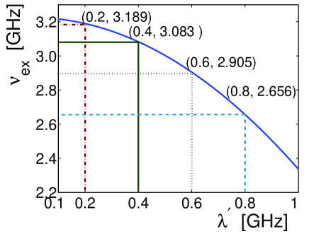
Figure 5: (Color online) To couple qubit to the LC circuit, the frequency $\nu_{ex}$, applied to the qubit, is plotted as a function of the coupling constant $\lambda^{\prime}$ between the qubit and the external microwave. As example, four different points are marked in the curve to show the required frequencies of external microwave when different coupling constants $\lambda^{\prime}$ are given.

A recent experiment ntt has demonstrated the Rabi oscillations between a single flux qubit and a superconducting LC circuit. In this experiment ntt , the coupling constant $g^{\prime}$ between the qubit and the LC circuit is about $g^{\prime}=0.2$ GHz, the qubit frequency $\nu_{q}$ at the optimal point is $\nu_{q}=2.1$ GHz, and the frequency of the LC circuit is $\nu_{LC}=4.35$ GHz. So the frequency difference between the LC circuit and the qubit is $\nu_{LC}-\nu_{q}=2.25$ GHz. The ratio $g^{\prime}/(\nu_{LC}-\nu_{q})$ of the coupling constant $g^{\prime}$ over the frequency difference $\nu_{LC}-\nu_{q}$ is about $0.089$. Therefore, the dispersive shift (or Lamb shift) of the LC circuit (qubit) due to nonresonantly interaction with the qubit (LC circuit) is about $0.018$ GHz.

If a TDEF with the frequency $\nu_{\rm ex}$ is applied to the qubit, then the TDEF and the qubit can form a dressed qubit with the frequency

$$\nu_{D}=\sqrt{(\nu_{\rm ex}-\nu_{q})^{2}+4|\lambda^{\prime}|^{2}}\,.$$ (39)

Here, the coupling constant between the qubit and the TDEF is $\lambda^{\prime}$. When the frequency $\nu_{D}$ of the dressed qubit satisfies the condition

$$\nu_{D}=\nu_{LC}-\nu_{\rm ex},$$ (40)

as shown in Eq. (13), then the dressed qubit can be resonantly coupled to the LC circuit. From the condition in Eq. (40), we derive another equation

$$\nu_{\rm ex}=\frac{1}{2}(\nu_{LC}+\nu_{q})-\frac{2|\lambda^{\prime}|^{2}}{(\nu_{LC}-\nu_{q})}.$$ (41)

To make the dressed qubit couple to the LC circuit, Eq. (41) shows that we should choose the different external frequencies $\nu_{\rm ex}$ for different coupling constants $\lambda^{\prime}$ when the frequencies of the data bus $\nu_{LC}$ and the qubit $\nu_{q}$ are given.

In Fig. 5, the frequency $\nu_{\rm ex}$ is plotted as a function of $\lambda^{\prime}$, which is in the interval $0.1\sim 1$ GHz, for the above given frequencies of the qubit and LC circuit. Figure 5 clearly shows that the frequencies $\nu_{\rm ex}$ of the applied external microwave are different for the different $\lambda^{\prime}$ in order to couple the qubit to the LC circuit with the assistance of the TDEF. As an example, four different points are marked in Fig. 5 to show the required frequencies $\nu_{\rm ex}$ of external microwave when the coupling constants $\lambda^{\prime}$ are different. For example, if $\lambda^{\prime}=0.4$ GHz, then the applied external microwave should have the frequency $\nu_{\rm ex}=3.083$ GHz to make the dressed qubit resonantly couple to the LC circuit. And then the effective coupling constant between the dressed qubit and the LC circuit is about $\kappa^{\prime}\approx 0.1996$ GHz for the coupling constant $g^{\prime}=0.2$ GHz between the qubit and the LC circuit. Therefore the microwave assisted resonant interaction between the qubit and the LC circuit can be realized in the current experimental setup ntt . Furthermore, this circuit can be also scaled up to many qubits.

VI.2 Charge qubit interacting with a single-mode cavity field

We consider another experimental example of a charge qubit interacting with a single-mode cavity field wallraff . In this experiment wallraff , the qubit frequency $\nu_{q}$ is about $8$ GHz at the degeneracy point. The frequency $\nu_{c}$ of the cavity field is about $6$ GHz. The coupling constant $g^{\prime}$ between the qubit and the cavity field can be, e.g., $50$ MHz, then the ratio between $g^{\prime}$ and the detuning $\nu_{q}-\nu_{c}$ is $g^{\prime}/(\nu_{q}-\nu_{c})=0.025$. This means that the qubit and the cavity field is in the large detuning regime.

If an ac electric field with frequency $\nu_{\rm ex}$ is applied to the gate of the charge qubit, then the qubit and the ac field can together form a dressed qubit. If we choose appropriate parameters for the ac field, the dressed qubit can be resonantly coupled to the cavity field and then the qubit and the cavity field can exchange information with the assistance of the ac field. For example, if the Rabi frequency of the qubit associated with the ac field is about, e.g., $\lambda^{\prime}\sim 100$ MHz, then the dressed qubit can be resonantly coupled to the cavity field when the frequency $\nu_{ex}$ of the ac field is $7.01$ GHz, which is obtained from Eq. (41).

For the above two examples, we need to stress that the bias of the “bare” charge or flux qubit is always kept to the optimal point during the operations. In the coupling process, the external microwave mixes the two “bare” qubit states, and the dressed qubit states are resonantly coupled to the data bus (an LC circuit or a single-mode cavity field).

VII Conclusion

In conclusion, using an example of a superconducting flux qubit interacting with an LC circuit–data bus, we study a method to couple and decouple selected qubits with the data bus. This method can be realized with the assistance of time-dependent electromagnetic fields (TDEFs). If a TDEF is applied to a selected qubit, then dressed qubit-TDEF states can be formed. By choosing appropriate parameters of the TDEF, the dressed qubit can interact resonantly with the data bus. However, when the TDEF is removed, then the qubit and the data bus are decoupled. By using this mechanism, many qubits can be selectively coupled to a data bus. Thus, quantum information can be transferred from one qubit to another through the data bus with the assistance of the TDEF.

We stress the following: (i) all qubits are decoupled from the data bus when their detunings to the data bus are far larger than their coupling constants to the LC circuit; (ii) the qubits can be independently manipulated by the TDEFs resonantly addressing them (for example, if $\omega_{m,c}=\omega_{m}$, then the $m$th qubit is addressed by its TDEF); (iii) to couple any one of the qubits to the data bus, an appropriate TDEF is needed to be applied such that the dressed qubit can be resonantly coupled to the data bus, and then the information of the qubit can be transferred to the data bus with the help of the TDEF.

We emphasize that all superconducting qubits (charge or flux qubits) can work at their optimal points during the coupling and decoupling processes with the assistance of the TDEF. Although this coupling/decoupling mechanism is mainly focused on superconducting flux qubits, it can also be applied to either charge (e.g, in Refs. you1 ; wallraff ), or phase martinis qubits, as well as other solid state systems. For instance, the coupling between two quantum-dot qubits can be switched on and off by using this method, or a large number of quantum-dot qubits can be scaled up by using a single-mode electromagnetic field with the assistance of the TDEF.

VIII acknowledgments

This work was supported in part by the National Security Agency (NSA) and Advanced Research and Development Activity (ARDA) under Air Force Office of Research (AFOSR) contract number F49620-02-1-0334; and also supported by the National Science Foundation grant No. EIA-0130383; and also supported by Army Research Office (ARO) and Laboratory of Physical Sciences (LPS). The work of C.P. Sun is also partially supported by the NSFC and FRP of China with No. 2001CB309310.

References

- (1) J. Q. You and F. Nori, Phys. Today 58 (11), 42 (2005); G. Wendin and V. S. Shumeiko, cond-mat/0508729.
- (2) Y. A. Pashkin, T. Yamamoto, O. Astafiev, Y. Nakamura, D. V. Averin, and J. S. Tsai, Nature 421, 823 (2003); T. Yamamoto, Y. A. Pashkin, O. Astafiev, Y. Nakamura, and J. S. Tsai, ibid. 425, 941 (2003);
- (3) J. B. Majer, F. G. Paauw, A. C. J. ter Haar, C. J. P. M. Harmans, and J. E. Mooij, Phys. Rev. Lett. 94, 090501 (2005).
- (4) B. L. T. Plourde, T. L. Robertson, P. A. Reichardt, T. Hime, S. Linzen, C. E. Wu, and J. Clarke, Phys. Rev. B 72, 060506(R) (2005).
- (5) A. Izmalkov, M. Grajcar, E. Ilichev, Th. Wagner, H. G. Meyer, A. Yu. Smirnov, M. H. S. Amin, A. M. van den Brink, and A. M. Zagoskin, Phys. Rev. Lett. 93, 037003 (2004); M. Grajcar, A. Izmalkov, S. H. W. van der Ploeg, S. Linzen, T. Plecenik, Th. Wagner, U. Huebner, E. Il’ichev, H. G. Meyer, A. Yu. Smirnov, Peter J. Love, Alec Maassen van den Brink, M. H. S. Amin, S. Uchaikin, A. M. Zagoskin, ibid. 96, 047006 (2006).
- (6) H. Xu, F. W. Strauch, S. K. Dutta, P. R. Johnson, R. C. Ramos, A. J. Berkley, H. Paik, J. R. Anderson, A. J. Dragt, C. J. Lobb, and F. C. Wellstood, Phys. Rev. Lett. 94, 027003 (2005).
- (7) A. J. Berkley, H. Xu, R. C. Ramos, M. A. Gubrud, F. W. Strauch, P. R. Johnson, J. R. Anderson, A. J. Dragt, C. J. Lobb, and F. C. Wellstood, Science 300, 1548 (2003).
- (8) R. McDermott, R. W. Simmonds, M. Steffen, K. B. Cooper, K. Cicak, K. D. Osborn, S. Oh, D. P. Pappas, and J. M. Martinis, Science 307, 1299 (2005).
- (9) Y. Makhlin, G. Schön, and A. Shnirman, Rev. Mod. Phys. 73, 357 (2001).
- (10) J. Q. You, C. H. Lam, and H. Z. Zheng Phys. Rev. B 63, 180501 (2001).
- (11) J. Q. You, J. S. Tsai, and F. Nori, Phys. Rev. Lett. 89, 197902 (2002).
- (12) J. Q. You and F. Nori, Phys. Rev. B 68, 064509 (2003); J. Q. You, J. S. Tsai, and F. Nori, Phys. Rev. B 68, 024510 (2003).
- (13) A. Blais, R. S. Huang, A. Wallraff, S. M. Girvin, and R. J. Schoelkopf, Phys. Rev A 69, 062320 (2004).
- (14) Y. X. Liu, L. F. Wei, and F. Nori, Europhys. Lett. 67, 941 (2004); Phys. Rev. A 71, 063820 (2005).
- (15) A. M. Zagoskin, M. Grajcar, and A. N. Omelyanchouk Phys. Rev. A 70, 060301 (2004); F. de Melo, L. Aolita, F. Toscano, and L. Davidovich, Phys. Rev. A 73, 030303(R) (2006).
- (16) R. Migliore and A. Messina, Phys. Rev. B 67, 134505 (2003).
- (17) A. Blais, A. Maassen van den Brink, and A. M. Zagoskin, Phys. Rev. Lett. 90, 127901 (2003).
- (18) A. N. Cleland and M. R. Geller, Phys. Rev. Lett. 93, 070501 (2004).
- (19) D. V. Averin and C. Bruder, Phys. Rev. Lett. 91, 057003 (2003).
- (20) B. L. T. Plourde, J. Zhang, K. B. Whaley, F. K. Wilhelm, T. L. Robertson, T. Hime, S. Linzen, P. A. Reichardt, C.-E. Wu, and J. Clarke, Phys. Rev. B 70, 140501(R) (2004).
- (21) C. Rigetti, A. Blais, and M. Devoret, Phys. Rev. Lett. 94, 240502 (2005).
- (22) Y. X. Liu, L. F. Wei, J. S. Tsai, and F. Nori, Phys. Rev. Lett. 96, 067003 (2006).
- (23) Y. X. Liu, L. F. Wei, J. S. Tsai, and F. Nori, cond-mat/0509236.
- (24) J. I. Cirac and P. Zoller, Phys. Rev. Lett. 74, 4091 (1995).
- (25) M. Sasura and V. Buzek, J. Mod. Opt. 49, 1593 (2002).
- (26) L. F. Wei, Y. X. Liu, and F. Nori, Phys. Rev. A 70, 063801 (2004).
- (27) A. Wallraff, D. I. Schuster, A. Blais, L. Frunzio, R. S. Huang, J. Majer, S. Kumar, S. M. Girvin, and R. J. Schoelkopf, Nature 431, 162 (2004).
- (28) I. Chiorescu, P. Bertet, K. Semba, Y. Nakamura, C. J. P. M. Harmans, and J.E. Mooij, Nature 431, 159 (2004).
- (29) P. Bertet, C. J. P. M. Harmans, J. E. Mooij, Phys. Rev. B 73, 064512 (2006).
- (30) A. O. Niskanen, Y. Nakamura, and J. S. Tsai, Phys. Rev. B 73, 094506 (2006).
- (31) F. Plastina and G. Falci, Phys. Rev. B 67, 224514 (2003).
- (32) J. Johansson, S. Saito, T. Meno, H. Nakano, M. Ueda, K. Semba, H. Takayanagi, Phys. Rev. Lett. 96, 127006 (2006).
- (33) O. Buisson and F. W. J. Hekking, in Macroscopic Quantum Coherence and Quantum Computing (Kluwer Academic, Dordrecht, 2001), pp. 137-145; F. W. J. Hekking, O. Buisson, F. Balestro, and M. G. Vergniory, cond-mat/0201284 (unpublished).
- (34) L. F. Wei, Y. X. Liu, and F. Nori, Europhys. Lett. 67, 1004 (2004); Phys. Rev. B 71, 134506 (2005).
- (35) Y. D. Wang, P. Zhang, D. L. Zhou, and C. P. Sun, Phys. Rev. B 70, 224515 (2004).
- (36) X. Zhou and A. Mizel, Physica C 432, 59 (2005).
- (37) T. P. Orlando, J. E. Mooij, L. Tian, C. H. van der Wal, L. S. Levitov, S. Lloyd, and J. J. Mazo, Phys. Rev. B 60, 15398 (1999).
- (38) Y. X. Liu, J. Q. You, L. F. Wei, C. P. Sun, and F. Nori, Phys. Rev. Lett. 95, 087001 (2005); Y. S. Greenberg, E. Il’ichev and A. Izmalkov, Europhys. Lett. 72, 880 (2005).
- (39) A. Maassen van den Brink, Phys. Rev. B 71, 064503 (2005).
- (40) Y. X. Liu, L. F. Wei, and F. Nori, Phys. Rev. A 72, 033818 (2005); C. P. Sun, L. F. Wei, Y. X. Liu, and F. Nori, quant-ph/0504056.
- (41) C. Cohen-Tannoudji, J. Dupont-Roc, and G. Grynberg, Atom-Photon Interactions (Wiley, New York, 1992).
- (42) K. B. Cooper, M. Steffen, R. McDermott, R. W. Simmonds, S. Oh, D. A. Hite, D. P. Pappas, and J. M. Martinis, Phys. Rev. Lett. 93, 180401 (2004).
- (43) David P. DiVincenzo, Phys. Rev. A 51, 1015 (1995).