Temperature and Disorder Chaos in three-dimensional Ising Spin Glasses

Abstract

We study the effects of small temperature as well as disorder perturbations on the equilibrium state of three-dimensional Ising spin glasses via an alternate scaling ansatz. By using Monte Carlo simulations, we show that temperature and disorder perturbations yield chaotic changes in the equilibrium state and that temperature chaos is considerably harder to observe than disorder chaos.

The fragility of the equilibrium state of random frustrated systems such as the Edwards-Anderson Ising spin glass Edwards and Anderson (1975); Mézard et al. (1987); Young (1998) has been predicted a long time ago McKay et al. (1982); Parisi (1984) and analyzed on the basis of scaling arguments Fisher and Huse (1986); Bray and Moore (1987). These scaling arguments predict that the configurations which dominate the partition function change drastically and randomly when the temperature or the disorder in the interactions between the spins are modified ever so slightly. The temperature chaos and disorder chaos effects have attracted considerable attention both from theory and experiment because of their potential relevance in explaining the spectacular rejuvenation and memory effects observed in hysteresis experiments in spin-glasses Nordblad and Svendlidh (1998); Dupuis et al. (2001); Jönsson et al. (2004) as well as other materials, such as random polymers and pinned elastic manifolds. Although there is evidence of disorder chaos in spin glasses, temperature chaos remains a controversial issue Kondor (1989); Ney-Nifle and Young (1997); Ney-Nifle (1998); Billoire and Marinari (2000, 2002), whereas for random polymers or pinned elastic objects Fisher and Huse (1991) chaos in general is well established Sales and Yoshino (2002); da Silveira and Bouchaud (2004); le Doussal (2005).

Despite this lack of consensus, it has been surmised that temperature chaos would only be observable in spin glasses at very large system sizes and for large temperature changes Aspelmeier et al. (2002); Rizzo and Crisanti (2003) thus making its presence unfathomable in simulations. These claims have recently been challenged. In particular, recent results point towards the existence of temperature chaos in four-dimensional Ising spin glasses Sasaki et al. (2005) where the free energy of a domain wall induced by a change in boundary conditions changes its sign chaotically with temperature in accordance with the droplet/scaling theories McKay et al. (1982); Fisher and Huse (1986); Bray and Moore (1987). In this work we study the overlap between states at different temperatures and disorder distributions directly for a physically relevant three-dimensional (3D) Ising spin glass. Our results show that the scaling laws that arise from the droplet theory are indeed well satisfied in 3D provided low enough temperatures are considered, although small corrections need to be applied. In addition, we show that temperature and disorder chaos have similar scaling functions. By rescaling the characteristic length scale in the problem, we show that disorder chaos appears at much shorter scales than temperature chaos

The paper is organized as follows: We discuss first the model and Monte Carlo methods used, followed by the disorder- and temperature-chaos scaling approaches. We conclude with the results of our simulations of the 3D Ising spin glass and a general discussion.

Model and numerical method

The Edwards-Anderson Edwards and Anderson (1975) Ising spin glass is given by the Hamiltonian

$${\mathcal{H}}=-\sum_{\langle ij\rangle}J_{ij}S_{i}S_{j},$$ (1)

where the Ising spins $S_{i}\in\{\pm 1\}$ are on a cubic lattice with $N=L^{3}$ vertices and the interactions $J_{ij}$ are Gaussian distributed random numbers with zero mean and standard deviation unity. The sum is over nearest neighbor pairs. The model undergoes a spin-glass transition at $T_{\rm c}=0.951(9)$ Bhatt and Young (1988); Marinari et al. (1998); Katzgraber et al. (2006).

The order parameter of the system is defined via the overlap between two copies $\alpha$ and $\beta$, i.e.,

$$q_{\alpha,\beta}=\frac{1}{N}\sum_{i=1}^{N}S^{\alpha}_{i}S^{\beta}_{i}.$$ (2)

Following previous studies Ney-Nifle and Young (1997); Ney-Nifle (1998), we probe temperature chaos when the temperature between both replicas is shifted by an amount $\Delta T$. Disorder chaos is studied by introducing a perturbation $\Delta J$ in the disorder, i.e.,

$$J_{ij}\rightarrow\tilde{J}_{ij}=\frac{J_{ij}+x\Delta J}{\sqrt{1+\Delta J^{2}}}$$ (3)

which leaves the disorder distribution invariant. In Eq. (3) $x$ is a Gaussian distributed random number with zero mean and standard deviation unity. To monitor the changes induced by the perturbations of the system, we compute the chaoticity parameter Ney-Nifle and Young (1997); Ney-Nifle (1998) given by

$$Q_{T_{1},T_{2}}=\left[\frac{\langle q^{2}_{T_{1},T_{2}}\rangle}{\sqrt{\langle q^{2}_{T_{1},T_{1}}\rangle\langle q^{2}_{T_{2},T_{2}}\rangle}}\right]_{\rm av}$$ (4)

for temperature chaos and by

$$Q_{\Delta J}=\left[\frac{\langle q^{2}_{J_{ij},\tilde{J}_{ij}}\rangle}{\langle q^{2}_{J_{ij},J_{ij}}\rangle}\right]_{\rm av}$$ (5)

for disorder chaos, respectively.

In Eqs. (4) and (5) $q^{2}$ is the square overlap, Eq. (2), between two copies at different temperature/disorder. Here $\langle\cdots\rangle$ represents a thermal average and $[\cdots]_{\rm av}$ represents a disorder average. In order to access low temperatures necessary to probe temperature chaos, we have used the parallel tempering Hukushima and Nemoto (1996); Marinari et al. (1996) Monte Carlo method in combination with the equilibration test presented in Ref. Katzgraber et al. (2001). Simulation parameters are listed in Table 1.

Table 1: Parameters of the simulation for each system size $L$. $N_{\rm samp}$ is the number of samples and $N_{\rm sw}$ is the total number of Monte Carlo sweeps used for equilibration for each of the $2N_{T}$ parallel tempering replicas for a single sample. An equal number of sweeps is used for measurement. The minimum temperature simulated is $T_{\rm min}=0.20$, the highest $T_{\rm max}=2.0$. For disorder chaos the disorder shifts used in Eq. (3) are $\Delta J=0.001$, $0.005$, $0.02$, $0.05$, $0.1$, $0.2$, and $0.5$. For temperature chaos we compute the overlap between $T_{\rm min}$ and $T_{i}$ with $i\in\{2,\ldots,N_{T}\}$ tem .

$L$	$N_{T}$	$N_{\rm samp}$	$N_{\rm sw}$
4	16	10000	262144
5	16	10000	262144
6	16	10000	262144
8	16	5000	1048576
10	22	2500	8388608

Disorder and Temperature Chaos

In what follows we discuss how chaos can arise in spin glasses using the early arguments presented in Refs. McKay et al. (1982), Fisher and Huse (1986), Bray and Moore (1987), and mea . Within the droplet theory framework Bray and Moore (1984); Fisher and Huse (1986), the low-lying excitations above the equilibrium state are obtained by flipping compact connected clusters of spins called droplets. A droplet of size $\ell$ has a fractal surface of dimension $d_{\rm s}<d$, and its excitation free energy $F>0$ is distributed via $P_{T}(F,\ell)=[\gamma(T)\ell]^{-\theta}\rho[F/\gamma(T)\ell^{\theta}]$, where $\rho(x)$ is a scaling function assumed to be nonzero at $x=0$ and which decays to zero for large $x$. The free-energy exponent $\theta$ is argued on general grounds to be such that $0<\theta\leq d_{\rm s}/2$ and $\gamma(T)$ is the free-energy stiffness (which goes to zero at $T_{\rm c}$). The droplet’s entropy $S$ can be written as $S=\sigma(T)\ell^{d_{\rm s}/2}$, where $\sigma$ is the entropy stiffness. Temperature chaos appears if the free energy of a droplet changes its sign when the temperature is modified. As noted in Refs. Fisher and Huse (1986) and Bray and Moore (1987), the length scale at which this happens can be estimated by noting that the energy of a droplet does not change much with temperature. Therefore, if one considers a droplet at temperature $T_{1}$ with free energy $F(T_{1})$, then at temperature $T_{2}>T_{1}$

$$F(T_{2})\approx F(T_{1})+T_{1}S(T_{1})-T_{2}S(T_{2}).$$ (6)

Because for typical droplets $F(T_{1})=\gamma(T_{1})\ell^{\theta}$ and $S=\sigma(T)\ell^{d_{\rm s}/2}$, the free energy excitation of such droplets becomes generally negative at temperature $T_{2}$ (so that the droplet has to be flipped) for length scales larger than the chaotic length Fisher and Huse (1986); Bray and Moore (1987) defined as

$$\ell_{{\rm c}}=\bigg{(}\frac{\gamma(T_{1})}{T_{2}~{}\sigma(T_{2})-T_{1}~{}\sigma(T_{1})}\bigg{)}^{1/{\zeta}}\;\;\text{with}\;\;\;\zeta=\frac{d_{\rm s}}{2}-\theta.$$ (7)

Usually, small temperature changes are studied such that $S(T_{1})\approx S(T_{2})$. Here however, we do not use this approximation and since in the low temperature phase, when one can define droplets, the entropy is proportional to $\sqrt{T}$ Fisher and Huse (1986); Aspelmeier et al. (2002), we write

$$\ell_{\rm c}(T_{1},T_{2})\propto\left(T_{2}^{3/2}-T_{1}^{3/2}\right)^{-1/\zeta}.$$ (8)

Equation (8) shows that when temperature is changed, equilibrium configurations are changed on scales greater than $\ell_{{\rm c}}$. Notice that by keeping the temperature dependence of the entropy, we obtain a slightly different scaling than usually considered Fisher and Huse (1986); Bray and Moore (1987), where a factor $\Delta T$ appears instead of $T_{2}^{3/2}-T_{1}^{3/2}$. While this makes no difference for small $\Delta T$ (which is the case in all simulations performed so far), this can be significant for temperature differences larger than the ones considered in this work. Similar arguments can also be applied to the case of a random perturbation in the disorder Fisher and Huse (1986); Bray and Moore (1987) – see for instance Ref. Krza̧kała and Bouchaud (2005) – where one obtains

$$\ell_{\rm c}(\Delta J)\propto\Delta J^{-1/\zeta}.$$ (9)

Considering system-size excitations, these arguments thus suggest that the chaoticity parameters defined in Eqs. (4) and (5) have the following scaling behavior

$$Q_{T_{1},T_{2}}(L,T_{1},T_{2}) = F_{T}[L/\ell_{\rm c}(T_{1},T_{2})],$$ (10)

$$Q_{\Delta J}(L,\Delta J) = F_{J}[L/\ell_{\rm c}(\Delta J)],$$

where $F(x)$ is a function with $F(0)=1$ that decays at large $x$. In what follows we test the aforementioned scaling relations via Monte Carlo simulations.

Numerical results

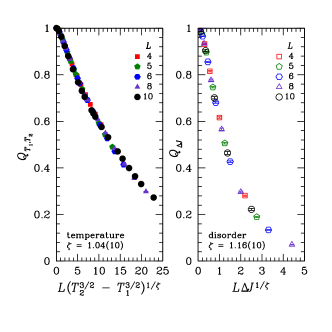
Figure 1: (Color online) Scaling plot of the chaoticity parameter for temperature chaos (left panel, $T_{1}=0.20$) and disorder chaos (right panel, $T=0.2$) using $L/\ell_{\rm c}$ as a scaling variable.

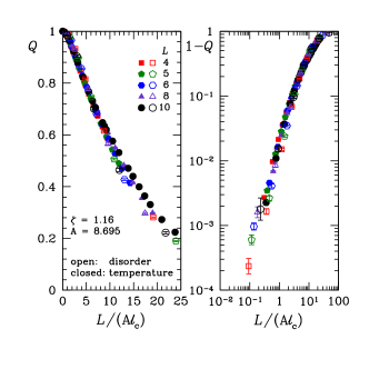
Figure 2: (Color online) Scaling plot of both disorder and temperature chaos. Left: Chaoticity parameter $Q$ as a function of $L/\ell_{\rm c}$. Scaling performed with $\zeta=1.16$. Note that $\ell_{\rm c}(\Delta T)\approx A\ell_{\rm c}(\Delta J)$ with $A\approx 8.7$, i.e., disorder chaos appears at considerably shorter length scales than temperature chaos. Right: Log-log plot of the same data, plotted as $1-Q$, to illustrate the quality of the scaling.

The behavior of the chaoticity parameter for disorder chaos at zero temperature has recently been studied in Ref. Krza̧kała and Bouchaud (2005) (see also Ref. Rieger et al. (1996)) and perfectly satisfies the predictions of the droplet model. We thus concentrate here on finite temperatures where the scaling relations were only tested in the simulations of Refs. Ney-Nifle and Young (1997), Ney-Nifle (1998), and Sasaki et al. (2005) in two and four space dimensions. We have performed low-temperature Monte Carlo simulations of the 3D Ising spin glass (see Table 1). As can be observed in Fig. 1, scaling the data for disorder and temperature chaos according to Eqs. (10) works extremely well. The best scaling collapse determined by a nonlinear minimization routine Katzgraber et al. (2006) yields $\zeta\approx 1.04$ for temperature chaos and $\zeta\approx 1.16$ for disorder chaos, which is in rather good agreement with the accepted value $\zeta\approx 1.1$ from $d_{\rm s}\approx 2.6$ Palassini and Young (2000); Katzgraber et al. (2001) and $\theta\approx 0.2$ Bray and Moore (1984); McMillan (1984); Hartmann (1999); see Eq. (7). Notice that we have a good scaling of the data even when $T_{2}$ is larger than $T_{\rm c}$. We have tested the temperature-dependence of the exponent $\zeta$ and find that for $T\leq 0.5$ its value is practically independent of temperature, i.e., at $T=0.20$ we are probing the low-temperature regime.

Renormalization group arguments also suggest that the temperature and disorder chaos effects are deeply related and characterized by the same universal scaling function Fisher and Huse (1986); Bray and Moore (1987); Sales and Yoshino (2002); da Silveira and Bouchaud (2004); le Doussal (2005) so that only nonuniversal prefactors differ. In Fig. 2, we thus superimpose the data for both perturbations presented in Fig. 1 by rescaling $\ell_{\rm c}$. Using $\zeta=1.16$ for both perturbations and multiplying $\ell_{\rm c}(\Delta J)$ by a factor $A\approx 8.7$, we obtain a rather good superposition in the low-temperature region, and we conclude that our data are thus compatible with the equality of the two scaling functions. From this $\ell$-scale renormalization we also conclude that the length scale at which temperature chaos appears is approximatively ten times larger than the length scale needed for disorder chaos to appear, as has also been found in four space dimensions by Sasaki et al., see Ref. Sasaki et al. (2005). Therefore temperature chaos is harder to probe than disorder chaos, as has already discussed within a Migdal-Kadanoff approach on spin glasses Aspelmeier et al. (2002).

The superposition of the scaling functions shows deviations at larger temperatures. This is not surprising as assumptions made when deriving the scaling function are not valid for high $T$. For example, the $\sqrt{T}$ dependence of the entropy or the very existence of droplets is only valid for $T\leq T_{c}$ Nifle and Hilhorst (1992). We thus believe that to perform a definitive test of universality of the scaling functions, very large system sizes at low temperatures with small temperature changes should be used.

We also study the behavior of the scaling function. It decays as $(\ell_{\rm c}/L)^{d/2}$ for strong chaos (when $\ell_{\rm c}/L\leq 1$) Krza̧kała and Bouchaud (2005). However, in the limit $\ell_{\rm c}/L\geq 1$, we obtain $1-Q(x)\propto x^{3\zeta/2}$ which differs from the $1-Q(x)\propto x^{\zeta}$ behavior found at zero temperature in Ref. Krza̧kała and Bouchaud (2005). This shows that the scaling function can have a more subtle behavior than what is naively expected from simple domain-wall arguments Sasaki et al. (2005); Scheffler et al. (2003). Note that the results remain unchanged if one takes the disorder average of the different overlaps in Eq. (4) independently, as done in Eq. (11) of Ref. Ney-Nifle (1998).

Finally, to better illustrate the mechanism of chaos, we study the distribution of the chaoticity parameter over the disorder for temperature chaos, i.e., we compute the chaoticity parameter $Q$ as defined in Eq. (4) without the disorder average, and bin the data for different choices of the disorder to compute the distribution $P_{L}(Q_{T_{1},T_{2}})$. According to the droplet model, in the weak chaos regime (where $\ell_{\rm c}>L$), temperature chaos can manifest itself even on small length scales, but only for rare regions of space Sales and Yoshino (2002). This means that even for small $\Delta T$, when Q is very close to unity, the distribution is broad and rare samples with lower values are expected. Figure 3 shows the distribution $P_{L}(Q_{T_{1},T_{2}})$ for $L=10$ for $T_{1}=0.2$ and different $T_{2}=T_{1}+\Delta T$ tem . Even for modest $\Delta T$, rare but large changes are clearly observed. This illustrates the weak chaos scenario presented in Ref. Sales and Yoshino (2002): temperature chaos (at least in the weak regime) is not due to moderate changes in all samples, but rather due to larger changes in a few rare samples.

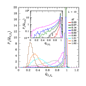
Figure 3: (Color online) Distribution of the chaoticity parameter over different realization of the disorder for $L=10$ with $T_{1}=0.2$ and $T_{2}=T_{1}+\Delta T$ tem . In the case of small $\Delta T$ rare samples have very low values of $Q$ while most of them remain unchanged ($Q=1$). The inset shows a linear-log plot of the data for the smallest values of $\Delta T$ for which $T_{1}<T_{2}<2T_{\rm c}/3$. For all $T_{2}$ the distribution has a single peak, unlike for the random-energy models with entropic fluctuations Krzakala and Martin (2002); Kurkova (2003).

Conclusions

We have studied numerically disorder and temperature chaos in 3D Ising spin glasses and show that both disorder as well as temperature chaos are well described within a scaling/droplet description. In particular, we find that the scaling variables have to be modified as done in Eq. (8) when the difference in temperature is large. In addition, we show that the weak chaos regime is dominated by rare events where system-size droplets are flipped. This has direct experimental implications because the weak chaos regime has been argued to account in a quantitative way for the memory and rejuvenation effects Jönsson et al. (2004). Finally, we show that temperature and disorder chaos might be described by similar scaling functions in the low-temperature regime, thus providing compelling evidence for the presence of a chaotic temperature dependence in spin glasses. This has also recently been proven for mean-field systems Rizzo and Yoshino (2006); Yoshino and Rizzo (2006). This mechanism is also responsible for step-size responses that could in principle be observed experimentally in mesoscopic systems Rizzo and Yoshino (2006); Yoshino and Rizzo (2006). Nevertheless, this behavior might change for larger system sizes and thus we propose to revisit the problem with better models Katzgraber et al. (2005). Our findings will help interpret experiments on rejuvenation and memory effects in spin-glasses and other materials.