Elasticity of a system with non-central potentials

Abstract

We derive expressions for determination of the stress and the elastic constants in systems composed of particles interacting via non-central two-body potentials as thermal averages of products of first and second partial derivatives of the interparticle potentials and components of the interparticle separation vectors. These results are adapted to hard potentials, when the stress and the elastic constants are expressed as thermal averages of the components of normals to contact surfaces between the particles and components of vectors separating the centers of the particles. The averages require the knowledge of simultaneous contact probabilities of two pairs of particles. We apply the expressions to particles for which a contact function can be defined, and demonstrate the feasibility of the method by computing the stress and the elastic constants of a two-dimensional system of hard ellipses using Monte Carlo simulations.

I Introduction

The mechanical response of materials to deformations is described by the elasticity theory lanlif . The simplest homogeneous (affine) deformation of a continuum can be expressed by a linear dependence of the distorted position ${\bf r}$ on the original position of that point ${\bf R}$ via relation

$$r_{i}=M_{ij}R_{j}\ ,$$ (1)

where $M_{ij}$ is a constant tensor. We will consider both two-dimensional (2D) and three-dimensional (3D) systems, in which Latin subscripts will indicate Cartesian coordinates. (Summation over repeated Latin subscripts is implied.) Tensor $M_{ij}$ can be separated into an identity tensor $I$ and a non-trivial part

$$M_{ij}=\delta_{ij}+\epsilon_{ij}\ .$$ (2)

In general, $\epsilon_{ij}$ can be separated into a symmetric tensor representing deformation and an anti-symmetric tensor representing rotation. We neglect the rotation and assume that $\epsilon_{ij}=\epsilon_{ji}$. While the tensor $\epsilon_{ij}$ has a convenient meaning in actual experiments, usually the elastic deformations are formulated in the terms of the Lagrangian strain tensor $\eta_{ij}$, which defines the change in the distances between the points etausage :

$$r_{i}r_{i}=M_{ik}M_{il}R_{k}R_{l}\equiv(\delta_{kl}+2\eta_{kl})R_{k}R_{l}\ .$$ (3)

In the case of affine deformations the definitions in Eqs. 1–3 are valid for arbitrarily values of $\epsilon_{ij}$ and $\eta_{ij}$. However, we will further assume that the deformations are small. For a homogeneous continuum, it suffices to apply the deformation described by Eq. 1 at the boundaries of the system to assure that the same equation describes every internal point, while in the case of inhomogeneous system, application of such a deformation to the boundaries assures that the mean deformation is equal to $\epsilon_{ij}$ hashin .

Elastic properties of a condensed matter system describe the energetic cost of a deformation. However, real system consisting of many moving atoms/molecules cannot be simply represented by a strain tensor assigned to every point in space. Rather, we can assume that the boundaries of such system undergo an affine deformation described by Eq. 1. In such a case, the mean free energy density, $f$, which is the free energy $F$ divided by the original (unstrained) volume $V_{0}$ of the system, can be expanded in a power series in the strain variables

$$f(\{\eta\})=f(\{0\})+\sigma_{ij}\eta_{ij}+\frac{1}{2}C_{ijkl}\eta_{ij}\eta_{kl}+\ldots$$ (4)

The coefficients in this expansion are the stress tensor $\sigma_{ij}$ and the tensor of the (second order) elastic constants $C_{ijkl}$, characterizing a given material. In the case of isotropic pressure $p$, the stress can be written as $\sigma_{ij}=-p\delta_{ij}$. Elastic constants may serve as an indicator of instabilities associated with phase transitions birch ; zhou .

Elastic response of a system to a deformation can be determined without actually distorting the system, since equilibrium correlation functions contain all the necessary information. Indeed almost four decades ago Squire, Holt and Hoover (SHH) shh developed a formalism that extended the theory of elasticity of Born and Huang born to a finite temperature situation and expressed the elastic properties of a system as thermal averages of various derivatives of interparticle potentials. In a certain sense the formalism is an extension of the virial theorem virtheorem which relates the thermal averages of the products of interparticle forces and the interparticle separations to the stress tensor. (Similar formalism enables evaluation of the elastic properties of 2D membranes in 3D space farago_pincus .) The SHH method is very well adapted for use in numerical simulations in constant volume (and shape) ensembles. Other methods, extracting the elastic properties from shape and volume changes of systems, have also been developed and extensively used other .

Usually molecules are not spherically symmetric and we may expect interactions that depend on the orientation of the molecules. The introduction of rotational degrees of freedom into the theoretical description of a system has an interesting effect on the stress and elastic constants. At very low densities (almost ideal gas) the rotational degrees of freedom add a large contribution to the total kinetic energy of a molecule, but do not contribute to the pressure. In a thermodynamical treatment of stress we are interested in the translational degrees of freedom. However, for non-spherically-symmetric potentials, the particle rotation may have a significant indirect contribution even at moderate densities. At larger densities phase diagram may be strongly influenced by those degrees of freedom. The general approach of SHH shh (see also Refs. zhou ; bavaud ) was applied in a detailed form to the case of particles interacting via central two-body forces. However, the formalism can be easily extended to the systems of particles interacting via non-central potentials, as will be shown in Section II.

Modelling of various systems frequently involves particles that interact via hard potentials which are either 0 or $\infty$: in fact simulation of 2D hard disk system dates back to the origins of the Metropolis Monte Carlo (MC) method origMetro . An obvious reason for the use of such potentials in simulations is their numerical simplicity. However, there are important physical reasons for such models: in many situations entropy plays a dominant role in physical processes, and the absence of energy scale in hard potentials “brings out” the entropic features of the behavior. Hard sphere systems have been the subject of an intensive research for several decades now (see gast and references therein). They serve as the simplest models for real fluids, glasses, and colloids. The phase diagram of hard spheres is well known. In 3D this system undergoes an entropically driven first-order phase transition from liquid to solid phase hsfreezing . Elastic constants of such solids have been explored in the past numres ; runge . Entropy also plays a crucial role in the systems containing long polymers, such as gels and rubbers polentropA ; degennes_polymer ; polentropB . Not surprisingly, hard sphere potentials have been extensively used to represent excluded volume interactions between the monomers (see baum and references therein). Kantor et al. kkn introduced tethering potential, that has no energy but limits the distance between bonded monomers, to represent covalent bonds in polymeric systems. Such hard potential combined with hard sphere repulsion can be used to simulate a variety of polymeric systems. Recently, Farago and Kantor fk_formalism adapted the formalism of SHH shh to hard potentials. This new formalism enabled a study of a sequence of entropy-dominated systems, such as 2D fk_2D and 3D fk_3D gels near sol-gel transition and other systems fk_net .

Orientation of non-spherically-symmetric molecules plays a crucial role in the properties of liquid crystals degennes_liquid . For instance, the nematic phase is translationally disordered but it has orientational order of the molecules. From the early stages of the liquid crystal research it has been realized that the entropic part of the free energy related to non-spherical shapes of the molecules, by itself, can explain many of the properties of the systems ons . Not surprisingly, hard potentials were frequently used to investigate the properties of liquid crystals. Even such simplifications as infinitely thin disks frenkel_thindisk or infinitely thin rods frenkel_thinrod provide valuable insights into the problem. A slightly more realistic picture is provided by hard spheroids fmm . Such simulations were primarily motivated by the desire to understand the liquid phases. However, two interesting solid phases have been detected: both phases are translationally ordered, but only one of them has orientational order of spheroids. The orientational order is absent only when the spheroid resembles a sphere. Sufficiently oblate or prolate spheroids are orientationally ordered in the solid phase. During the last twenty years hard spheroids have be studied in great detail spheroids . A similar hard potential system that is suitable for the study of the liquid crystals is a collection of hard spherocylinders (cylinders capped at their ends by hemispheres). These molecules have slightly more complex phase diagram (which includes smectic-A liquid-crystalline phase), and also have been studied in great detail spherocyl . Like spheroids, they have two solid phases. (Spherocylinders do not have a shape resembling oblate spheroid.) Taken together, spheroids and spherocylinders provide a rather coherent picture of influence of molecular shape on the phase diagram (see, e.g., sp ). Hard potentials also have been used in other ways to represent non-spherically symmetric molecules by combining several spheres or disks into more complicated shapes, such as heptagons woj , or long rods hardlong . To make the models more realistic, sometimes attractive interaction has been added to the usual hard repulsive potential attr .

In Section II we present the formalism for soft non-central pair potentials. This formalism cannot be directly applied to the calculation of elastic constants of hard potential systems. In Section III and Appendix A we show how generalization of the approach used for centrally-symmetric hard potentials fk_formalism can be used to derive expressions applicable to non-central hard potentials. In Section IV we detail the method by which the formal results can be applied to hard particles for which a “contact function” can be defined. In particular, we describe how our formalism can be used for a 2D system of hard ellipses. In Section V we demonstrate the implementation by calculating stress and elastic constants in different phases of a system of hard ellipses.

II Elastic properties for soft pair potentials

In this section we derive explicit expressions for the stress and elastic constant tensors following the method of SHH shh for a more general case. We will consider potential energy $\cal V$ which can be expressed as

$${\cal V}=\sum_{\langle\alpha\beta\rangle}\Phi({\bf r}^{\alpha\beta},\Omega^{\alpha},\Omega^{\beta}),$$ (5)

where $\Phi$ is the interaction potential of a pair of particles. Greek indices $\alpha$ and $\beta$ denote particles (atoms/molecules), and $\langle\alpha\beta\rangle$ denotes a pair of particles. The above equation contains summation over all possible particle pairs. (In this paper we do not assume summation over repeated Greek indices indicating particles.) Here ${\bf r}^{\alpha\beta}={\bf r}^{\beta}-{\bf r}^{\alpha}$ is the vector connecting two particles, while $\Omega^{\alpha}$ is the orientation of particle $\alpha$. The two-body potential is not necessarily spherically symmetric. In fact, we will apply our results to particles that do not posses such a symmetry. We denote all two-body potentials by the same letter $\Phi$ although nowhere in this formal derivation it is required that they should be identical for different pairs of particles. (It should be denoted $\Phi^{\alpha\beta}({\bf r}^{\alpha\beta},\Omega^{\alpha},\Omega^{\beta})$; however, we omit the superscript of $\Phi$ for brevity.) From the physical point of view we expect that the potential should be rotationally invariant, i.e. when the vector ${\bf r}^{\alpha\beta}$ and the orientations of two molecules (described by $\Omega^{\alpha}$ and $\Omega^{\beta}$) perform a “rigid body” rotation, the interaction energy should not change. In fact the symmetry of the stress tensor assumes the presence of rotational invariance. However, we do not explicitly use this property in the derivation of the following expressions.

Unlike the central force case shh we will need to use both $\eta_{ij}$ and $\epsilon_{ij}$ in the process of derivation. Note that in the definition of $\eta_{ij}$ in Eq. 3 only the symmetric sum $\eta_{ij}+\eta_{ji}$ appears for $i\neq j$. Therefore, without loss of generality it is assumed that the Lagrangian strain is a symmetric tensor ($\eta_{ij}=\eta_{ji}$). From Eqs. 2 and 3 we find that $\eta_{kl}=\frac{1}{2}(\epsilon_{kl}+\epsilon_{lk}+\epsilon_{ik}\epsilon_{il})$. For small deformations this relation can be inverted to the second order as

$$\epsilon_{kl}=\eta_{kl}-\frac{1}{2}\eta_{mk}\eta_{ml}+\dots$$ (6)

In statistical-mechanical description of a solid in a canonical ensemble we may ask how the free energy $F$ of the solid changes when the boundaries of the solid undergo deformation described by Eq. 1. In calculation of such $F(\{\eta\})$ we do not impose any restrictions on the positions or orientations of the particles except the change in the boundary conditions. The free energy can be expressed via the partition function as

$$F(\{\eta\})=-kT\ln[Z_{0}Z(\{\eta\})],$$ (7)

where only the configurational part $Z(\{\eta\})$ of the partition depends on the deformation, while the remaining (“kinetic”) part $Z_{0}$ is independent of deformations. We note, that in classical physics the details of the inertia tensors of the molecules can modify the details of their actual motion, but play no role in the statistical-mechanical properties of the system. Only the asphericity of the potential matters. The configurational part

$$Z=\int\limits_{V(\{\eta\})}\prod_{\lambda=1}^{N}d{\bf r}^{\lambda}\int\prod_{\lambda=1}^{N}d\Omega^{\lambda}\ {\rm e}^{-{\cal V}({\bf r}^{1},\Omega^{1},\dots,{\bf r}^{N},\Omega^{N})/kT},$$ (8)

where ${\bf r}^{\alpha}$ and $\Omega^{\alpha}$ represent the position and orientation of particle $\alpha$ and $\cal V$ is the interaction potential, depends on the deformation only through the distortion of the integration volume $V(\{\eta\})$ of the possible positions of each of the particles. The integration over all possible spatial directions of each particle remains unchanged. If we formally change the integration variable ${\bf r}^{\alpha}$ for each particle $\alpha$ to the variable ${\bf R}^{\alpha}$, which are related by Eq. 1, then, the limits of interaction of the new variables will correspond to the undistorted volume $V(\{0\})\equiv V_{0}$, and consequently

$$Z=\int\limits_{V_{0}}\prod_{\lambda=1}^{N}d{\bf r}^{\lambda}\int\prod_{\lambda=1}^{N}d\Omega^{\lambda}J{\rm e}^{-{\cal V}(M_{ij}R^{1}_{j},\Omega^{1},\dots,M_{ij}R^{N}_{j},\Omega^{N})/kT},$$ (9)

where $J$ is the Jacobian corresponding to the change of coordinates

$$J=|\det(M)|^{N}=|\det(I+2\eta)|^{N/2}\ .$$ (10)

The deformation now appears as distortion of the coordinates in the potential $\cal V$.

Thus, the stress and the elastic constants can be viewed as the first and the second derivatives of the free energy density with respect to various $\eta_{ij}$. Since in the expansion in Eq. 4 always appear pairs of terms such as $C_{1123}\eta_{11}\eta_{23}+C_{1132}\eta_{11}\eta_{32}$ which contain identical $\eta$ terms, we can choose to define the tensor in a symmetric form $C_{ijkl}=C_{jikl}=C_{ijlk}$. (An additional symmetry $C_{ijkl}=C_{klij}$ is also evident from the definition of the tensor.) Strictly speaking, since $\eta_{12}=\eta_{21}$ they should be treated as a single variable while taking the derivatives of the free energy density. However, terms containing those two variables also appear twice in Eq. 4. Thus, one can simply treat $\eta_{12}$ and $\eta_{21}$ as independent variables, and symmetrize the results with the interchange of indices at the end. Alternatively, one may view each derivative $\partial/\partial\eta_{12}$ as $\frac{1}{2}(\partial/\partial\eta_{12}+\partial/\partial\eta_{21})$. Below we always present fully symmetrized expressions.

From Eqs. 4 and 7 we can express the stress tensor

$$V_{0}\sigma_{ij}=\frac{\partial{F}}{\partial{\eta_{ij}}}\biggm{|}_{\{\eta\}=\{0\}}=-\frac{kT}{Z}\frac{\partial{Z}}{\partial{\eta_{ij}}}\biggm{|}_{\{\eta\}=\{0\}}$$ (11)

and the second order elastic constants

$$V_{0}C_{ijmn}=\frac{\partial^{2}F}{\partial\eta_{mn}\partial\eta_{ij}}\biggm{|}_{\{\eta\}=\{0\}}$$

$$=\left[\frac{kT}{Z^{2}}\frac{\partial{Z}}{\partial{\eta_{mn}}}\frac{\partial{Z}}{\partial{\eta_{ij}}}-\frac{kT}{Z}\frac{\partial^{2}{Z}}{\partial{\eta_{mn}}\partial{\eta_{ij}}}\right]\biggm{|}_{\{\eta\}=\{0\}}$$ (12)

in terms of the derivatives of $Z$. As can be seen from Eq. 9 the dependence of $Z$ on the deformation is contained in the Jacobian $J$ and in the arguments of the potential $\cal V$. The Jacobian depends directly on $\eta_{ij}$ and its derivatives can be easily calculated. In particular, we find (see, e.g., Ref. fk_formalism ) that

$$\frac{\partial J}{\partial\eta_{ij}}\biggm{|}_{\{\eta\}=\{0\}}=N\delta_{ij}$$ (13)

$$\frac{\partial^{2}J}{\partial\eta_{mn}\partial\eta_{ij}}\biggm{|}_{\{\eta\}=\{0\}}=N^{2}\delta_{ij}\delta_{mn}-N\delta_{im}\delta_{jn}-N\delta_{in}\delta_{jm}.$$ (14)

Taking the derivatives of $\cal V$ involves the differentiation of the potential with respect to $M_{ij}$, followed by the differentiation of $M_{ij}$ with respect to $\epsilon_{kl}$ using Eq. 2, followed by the differentiation of $\epsilon_{kl}$ with respect to $\eta_{mn}$ using Eq. 6. This leads to the following expressions for the stress and elastic constants:

$$V_{0}\sigma_{ij}=-NkT\delta_{ij}+\frac{1}{2}\sum_{\langle\alpha\beta\rangle}\left\langle\frac{\partial\Phi\ }{\partial R^{\alpha\beta}_{i}}R^{\alpha\beta}_{j}+\frac{\partial\Phi\ }{\partial R^{\alpha\beta}_{j}}R^{\alpha\beta}_{i}\right\rangle\ ,$$ (15)

$$V_{0}C_{ijmn}=NkT(\delta_{im}\delta_{jn}+\delta_{in}\delta_{jm})$$ (16)

$$+ \frac{1}{4kT}\sum_{\langle\alpha\beta\rangle}\left\langle\frac{\partial\Phi}{\partial R^{\alpha\beta}_{i}}R^{\alpha\beta}_{j}+\frac{\partial\Phi}{\partial R^{\alpha\beta}_{j}}R^{\alpha\beta}_{i}\right\rangle\sum_{\langle\gamma\delta\rangle}\left\langle\frac{\partial\Phi}{\partial R^{\gamma\delta}_{m}}R^{\gamma\delta}_{n}+\frac{\partial\Phi}{\partial R^{\gamma\delta}_{n}}R^{\gamma\delta}_{m}\right\rangle$$

$$- \frac{1}{4kT}\sum_{\langle\alpha\beta\rangle,\langle\gamma\delta\rangle}\Bigg{\langle}\frac{\partial\Phi}{\partial R^{\alpha\beta}_{m}}\frac{\partial\Phi}{\partial R^{\gamma\delta}_{i}}R^{\alpha\beta}_{n}R^{\gamma\delta}_{j}+\frac{\partial\Phi}{\partial R^{\alpha\beta}_{n}}\frac{\partial\Phi}{\partial R^{\gamma\delta}_{i}}R^{\alpha\beta}_{m}R^{\gamma\delta}_{j}+\frac{\partial\Phi}{\partial R^{\alpha\beta}_{m}}\frac{\partial\Phi}{\partial R^{\gamma\delta}_{j}}R^{\alpha\beta}_{n}R^{\gamma\delta}_{i}+\frac{\partial\Phi}{\partial R^{\alpha\beta}_{n}}\frac{\partial\Phi}{\partial R^{\gamma\delta}_{j}}R^{\alpha\beta}_{m}R^{\gamma\delta}_{i}\Bigg{\rangle}$$

$$+ \frac{1}{4}\sum_{\langle\alpha\beta\rangle}\Bigg{\langle}\frac{\partial^{2}\Phi}{\partial R^{\alpha\beta}_{m}\partial R^{\alpha\beta}_{i}}R^{\alpha\beta}_{n}R^{\alpha\beta}_{j}+\frac{\partial^{2}\Phi}{\partial R^{\alpha\beta}_{n}\partial R^{\alpha\beta}_{i}}R^{\alpha\beta}_{m}R^{\alpha\beta}_{j}+\frac{\partial^{2}\Phi}{\partial R^{\alpha\beta}_{m}\partial R^{\alpha\beta}_{j}}R^{\alpha\beta}_{n}R^{\alpha\beta}_{i}+\frac{\partial^{2}\Phi}{\partial R^{\alpha\beta}_{n}\partial R^{\alpha\beta}_{j}}R^{\alpha\beta}_{m}R^{\alpha\beta}_{i}\Bigg{\rangle}$$

$$- \frac{1}{8}\sum_{\langle\alpha\beta\rangle}\Bigg{\{}\left\langle\frac{\partial\Phi}{\partial R^{\alpha\beta}_{j}}R^{\alpha\beta}_{n}+\frac{\partial\Phi}{\partial R^{\alpha\beta}_{n}}R^{\alpha\beta}_{j}\right\rangle\delta_{im}+\left\langle\frac{\partial\Phi}{\partial R^{\alpha\beta}_{i}}R^{\alpha\beta}_{m}+\frac{\partial\Phi}{\partial R^{\alpha\beta}_{m}}R^{\alpha\beta}_{i}\right\rangle\delta_{jn}$$

$$+ \left\langle\frac{\partial\Phi}{\partial R^{\alpha\beta}_{i}}R^{\alpha\beta}_{n}+\frac{\partial\Phi}{\partial R^{\alpha\beta}_{n}}R^{\alpha\beta}_{i}\right\rangle\delta_{jm}+\left\langle\frac{\partial\Phi}{\partial R^{\alpha\beta}_{j}}R^{\alpha\beta}_{m}+\frac{\partial\Phi}{\partial R^{\alpha\beta}_{m}}R^{\alpha\beta}_{j}\right\rangle\delta_{in}\Bigg{\}}\ .$$

In the above equations we already use the coordinates $\bf R^{\alpha\beta}$ of the undistorted system to emphasize the fact that all the averages are now calculated in the absence of the deformation.

Since $(\partial\Phi/\partial R^{\alpha\beta}_{i})R^{\alpha\beta}_{j}=-f^{\alpha\beta}_{i}R^{\alpha\beta}_{j}$, where ${\bf f}^{\alpha\beta}$ is the force between the particles $\alpha$ and $\beta$, we can recognize in Eq. 15 the standard virial theorem, although in the textbooks virtheorem the derivation is quickly reduced to calculation of the (isotropic) pressure $p$.

The accuracy of the expressions 15 and 16 can be verified by reducing the above formulae to the case of isotropic central force potential in which case

$$\frac{\partial\Phi}{\partial R_{i}}=\Phi^{\prime}\frac{R_{i}}{R}\ ,$$ (17)

where prime denotes a derivative of $\Phi$ with respect to inter-particle separation $R$. Similarly,

$$\frac{\partial^{2}\Phi}{\partial R_{i}\partial R_{j}}=\Phi^{\prime\prime}\frac{R_{i}R_{j}}{R^{2}}+\Phi^{\prime}\frac{\delta_{ij}}{R}-\Phi^{\prime}\frac{R_{i}R_{j}}{R^{3}}$$ (18)

After performing these substitutions, we recover the standard expressions for central force potentials shh .

III Hard potentials

Figure 1: Two “hard” particles at a close approach. ${\bf R}^{\alpha\beta}$ is a vector connecting their centers, and $s^{\alpha\beta}$ is the minimal separation of the surfaces.

The expressions for stress and elastic constants that have been obtained in the previous section, presumed smooth potentials with well defined first and second derivatives. There is a certain difficulty in translating the expressions obtained for soft potentials to a hard potential situation. For instance, the term $(\partial\Phi/\partial R^{\alpha\beta}_{i})R^{\alpha\beta}_{j}$ in Eq. 15 looks poorly defined for a hard potential that changes on contact between 0 and $\infty$. However, we note that the derivative of the potential really originates from the derivative $\partial[{\rm e}^{-\Phi({\bf R}^{\alpha\beta},\Omega^{\alpha},\Omega^{\beta})/kT}]/\partial R^{\alpha\beta}_{i}$. The latter, is a derivative of a step function that changes between 0 and 1, when the potential changes between $\infty$ and 0. This observation, has been used in Refs. runge ; barker to derive simple expressions for the pressure of hard sphere system. A detailed and rigorous description of the various aspects (including calculation of pressure) of interaction of hard convex solids can be found in Ref. hardpotreview . A typical interaction between two hard particles (e.g., ellipses in 2D or ellipsoids in 3D) is represented by Fig. 1 which depicts a close approach of two such particles, when ${\bf R}^{\alpha\beta}$ is the vector connecting their centers, while $s^{\alpha\beta}$ denotes the minimal distance between them. Gradient of ${\rm e}^{-\Phi({\bf R}^{\alpha\beta},\Omega^{\alpha},\Omega^{\beta})/kT}$ with respect to ${\bf R}^{\alpha\beta}$, when $\Omega^{\alpha}$ and $\Omega^{\beta}$ are kept fixed, is simply ${\bf n}^{\alpha\beta}\delta(s^{\alpha\beta})$ where ${\bf n}^{\alpha\beta}$ is unit vector perpendicular to the surfaces at the point of contact, pointing from $\alpha$ to $\beta$. Thus we can make the substitution

$$\left\langle\frac{\partial\Phi}{\partial R^{\alpha\beta}_{i}}R^{\alpha\beta}_{j}\right\rangle\rightarrow-kT\int d{\bf R}^{\alpha}d{\bf R}^{\beta}d\Omega^{\alpha}d\Omega^{\beta}\times$$

$$n^{\alpha\beta}_{i}\delta(s^{\alpha\beta})R^{\alpha\beta}_{j}P({\bf R}^{\alpha},\Omega^{\alpha},{\bf R}^{\beta},\Omega^{\beta})$$ (19)

where

$$P({\bf R}^{\alpha},\Omega^{\alpha},{\bf R}^{\beta},\Omega^{\beta})=$$

$$\frac{1}{Z}\int\prod_{\lambda=1\atop\lambda\neq\alpha,\beta}^{N}(d{\bf R}^{\lambda}d\Omega^{\lambda}){\rm e}^{-\sum_{\langle\mu\nu\rangle\atop\neq\langle\alpha\beta\rangle}\Phi({\bf R}^{\mu\nu},\Omega^{\mu},\Omega^{\nu})/kT}$$ (20)

is the probability density of particles $\alpha$ and $\beta$ to be at particular positions and orientations. The integral in Eq. III simply represents the average of $n^{\alpha\beta}_{i}R^{\alpha\beta}_{j}$ over all possible contacts between two particles weighted with proper probability densities of those contacts. (Since the probability density changes from a finite value, when the particles are almost in contact, to zero, when the particles overlap, we need to consider the case when $s^{\alpha\beta}$ approaches 0 from the positive side.) Thus, if we denote $\Delta_{i}^{\alpha\beta}=n^{\alpha\beta}_{i}\delta(s^{\alpha\beta}-0^{+})$, we can find the hard potential limit by replacement

$$\frac{\partial\Phi}{\partial R^{\alpha\beta}_{i}}\rightarrow-kT\Delta_{i}^{\alpha\beta}$$ (21)

By substituting the result into Eq. 15 we obtain the following expression for the stress in the case of hard potentials:

$$\frac{V_{0}\sigma_{ij}}{kT}=-N\delta_{ij}-\frac{1}{2}\sum_{\langle\alpha\beta\rangle}\left\langle\Delta_{i}^{\alpha\beta}R^{\alpha\beta}_{j}+\Delta_{j}^{\alpha\beta}R^{\alpha\beta}_{i}\right\rangle.$$ (22)

The substitution appearing in Eq. 21 cannot be used to calculate the elastic constants in Eq. 16, since the latter expression contains a double summation (over pairs $\langle\alpha\beta\rangle$ and $\langle\gamma\delta\rangle$) of the derivatives of the potentials. Such summation includes a term where $\langle\alpha\beta\rangle=\langle\gamma\delta\rangle$. A direct substitution of Eq. 21 would lead to the appearance of the term $[\delta(s^{\alpha\beta})]^{2}$ which causes the expression to diverge. (This is a true divergence, rather than some mathematical subtlety of approaching the limit of hard potentials.) However, Eq. 16 also contains the second derivative of $\Phi$, which becomes poorly defined in the hard potential limit. We shall show in the Appendix A that the sum of the apparently divergent and poorly defined terms has a well defined hard potential limit. In fact this sum can be transformed into an expression in Eq. 32 which includes only first derivatives of potentials and products of the first derivatives of potentials of different particle pairs. While the resulting expression in Eq. 32 looks more complicated, it can be simply transformed (using Eq. 21) into an expression for the elastic constants of hard particles:

$$\frac{V_{0}C_{ijmn}}{kT} = N(\delta_{im}\delta_{jn}+\delta_{in}\delta_{jm})$$ (23)

$$+ \frac{1}{4}\sum_{\langle\alpha\beta\rangle}\left\langle\Delta_{i}^{\alpha\beta}R^{\alpha\beta}_{j}+\Delta_{j}^{\alpha\beta}R^{\alpha\beta}_{i}\right\rangle\sum_{\langle\gamma\delta\rangle}\Big{\langle}\Delta_{m}^{\gamma\delta}R^{\gamma\delta}_{n}+\Delta_{n}^{\gamma\delta}R^{\gamma\delta}_{m}\Big{\rangle}$$

$$- \frac{1}{4}\sum_{\langle\alpha\beta\rangle}\sum_{\langle\gamma\delta\rangle\atop\neq\langle\alpha\beta\rangle}\left\langle\Delta_{m}^{\alpha\beta}\Delta_{i}^{\gamma\delta}R^{\alpha\beta}_{n}R^{\gamma\delta}_{j}+\Delta_{n}^{\alpha\beta}\Delta_{i}^{\gamma\delta}R^{\alpha\beta}_{m}R^{\gamma\delta}_{j}+\Delta_{m}^{\alpha\beta}\Delta_{j}^{\gamma\delta}R^{\alpha\beta}_{n}R^{\gamma\delta}_{i}+\Delta_{n}^{\alpha\beta}\Delta_{j}^{\gamma\delta}R^{\alpha\beta}_{m}R^{\gamma\delta}_{i}\right\rangle$$

$$+ \frac{1}{8}\sum_{\langle\alpha\beta\rangle}\sum_{\gamma\atop\neq\alpha,\beta}\Big{\langle}\Delta_{m}^{\alpha\beta}\left(\Delta_{i}^{\gamma\beta}+\Delta_{i}^{\alpha\gamma}\right)R^{\alpha\beta}_{n}R^{\alpha\beta}_{j}+\Delta_{n}^{\alpha\beta}\left(\Delta_{i}^{\gamma\beta}+\Delta_{i}^{\alpha\gamma}\right)R^{\alpha\beta}_{m}R^{\alpha\beta}_{j}$$

$$+ \Delta_{m}^{\alpha\beta}\left(\Delta_{j}^{\gamma\beta}+\Delta_{j}^{\alpha\gamma}\right)R^{\alpha\beta}_{n}R^{\alpha\beta}_{i}+\Delta_{n}^{\alpha\beta}\left(\Delta_{j}^{\gamma\beta}+\Delta_{j}^{\alpha\gamma}\right)R^{\alpha\beta}_{m}R^{\alpha\beta}_{i}\Big{\rangle}$$

$$+ \frac{1}{4}\sum_{\langle\alpha\beta\rangle}\Big{\{}\left\langle\Delta_{j}^{\alpha\beta}R^{\alpha\beta}_{n}+\Delta_{n}^{\alpha\beta}R^{\alpha\beta}_{j}\right\rangle\delta_{im}+\left\langle\Delta_{i}^{\alpha\beta}R^{\alpha\beta}_{m}+\Delta_{m}^{\alpha\beta}R^{\alpha\beta}_{i}\right\rangle\delta_{jn}+\left\langle\Delta_{i}^{\alpha\beta}R^{\alpha\beta}_{n}+\Delta_{n}^{\alpha\beta}R^{\alpha\beta}_{i}\right\rangle\delta_{jm}$$

$$+ \left\langle\Delta_{j}^{\alpha\beta}R^{\alpha\beta}_{m}+\Delta_{m}^{\alpha\beta}R^{\alpha\beta}_{j}\right\rangle\delta_{in}+\left\langle\Delta_{m}^{\alpha\beta}R^{\alpha\beta}_{n}+\Delta_{n}^{\alpha\beta}R^{\alpha\beta}_{m}\right\rangle\delta_{ij}+\left\langle\Delta_{i}^{\alpha\beta}R^{\alpha\beta}_{j}+\Delta_{j}^{\alpha\beta}R^{\alpha\beta}_{i}\right\rangle\delta_{mn}\Big{\}}.$$

Each of the terms in the above equation corresponds to some particular case of contact between pairs of particles. E.g., term of the type $\langle\Delta_{i}^{\alpha\beta}R^{\alpha\beta}_{j}\rangle$ in the last sum corresponds to a contact between a pair of particles $\alpha$ and $\beta$, and consequently the contribution of that sum is proportional to $N$. The sum with the prefactor $\frac{1}{8}$ contains terms corresponding to three touching particles: E.g., the term $\langle\Delta_{m}^{\alpha\beta}\Delta_{i}^{\gamma\beta}R^{\alpha\beta}_{n}R^{\alpha\beta}_{j}\rangle$ corresponds to the situation when particle $\beta$ touches particles $\alpha$ and $\gamma$ simultaneously. The number of such contacts at any given moment is also proportional to $N$. The second and the third lines of the equation have $N^{2}$ different averages corresponding to the number of pairs of contacts that might appear in the system. However, we note that in both sums taken together we always have differences of the type $\langle\Delta_{i}^{\alpha\beta}R^{\alpha\beta}_{j}\rangle\langle\Delta_{m}^{\gamma\delta}R^{\gamma\delta}_{n}\rangle-\langle\Delta_{i}^{\alpha\beta}R^{\alpha\beta}_{j}\Delta_{m}^{\gamma\delta}R^{\gamma\delta}_{n}\rangle$. This term vanishes if the contact between the pair $\langle\alpha\beta\rangle$ is uncorrelated with the contact between the pair $\langle\gamma\delta\rangle$. This happens when the two pairs are outside the correlation distance. Consequently, only pairs of contacts close to each other will contribute, and therefore the total contribution of those terms is proportional to $N$.

IV Application to hard ellipse system

Equations 22 and 23 enable calculation of the stress and elastic constants of a system consisting of hard particles, provided we are able to calculate thermal averages of the type $\langle\Delta_{i}^{\alpha\beta}R^{\alpha\beta}_{j}\rangle$. This expression depends on the probability density of particles being in contact. For the calculation of stress we need only the probability density of a single contact between a pair of particles, while the calculation of elastic constants involves the probability density of two such contacts happening simultaneously. It is natural to use MC method hoover_bk ; frenkel_bk ; binder_bk to evaluate averages of this type. MC simulation of hard potentials is particularly simple since no energy scale is present, and every elementary move of a particle is either accepted without a need to calculate the Boltzmann factor, or results in a forbidden configuration, and is, consequently, rejected. Application, of these procedures requires a method to identify intersection of two hard particles. Such methods have been found both for 2D ellipses vieillard and for 3D ellipsoids hard_spheroids_funct ; perram . In Appendix B we explain in detail the case of ellipses which is used in the current work. Here, we will consider a slightly more general case when a simple function can be defined that identifies the contact between two particles.

Consider a function $\Psi$ that depends on the positions and orientations of two particles, that vanishes when the particles touch each other and is positive when the particles are separated. (The formalism can be trivially generalized to the case when the the function has some other non-vanishing constant value at the contact.) Consider a case when the orientations of both particles are fixed, and we explore positions where the function vanishes. Figs. 2a and 2b depict 2D cases of one fixed ellipse, while another (identical) ellipse is rotated by a fixed angle and is shown in a variety positions where they touch. The ratio between the major and minor semi-axes of the ellipses, $a$ and $b$, respectively, are different in both pictures. The thick line traces the possible positions of the center of the moving ellipse. Note that the shape of such a contact line depends on the degree of elongation of the ellipses and on their relative orientation. Those are the positions that are relevant for the calculation of the average $\langle\Delta_{i}^{\alpha\beta}R^{\alpha\beta}_{j}\rangle$. In 2D this is a line, while in 3D this is a surface.

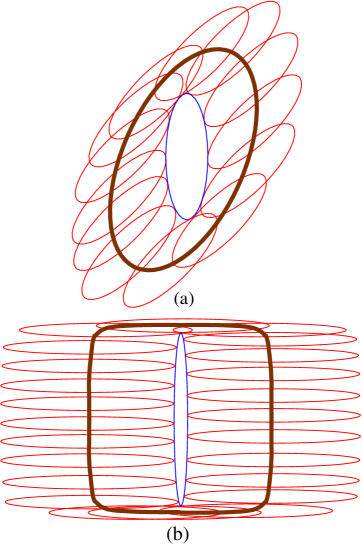
Figure 2: (a) Center of slightly elongated ellipse ($a/b=3$) tilted by 45^o with respect to an identical (vertical) ellipse circumscribes an “oval” trajectory, depicted by the thick line, when the contact point moves along the ellipse. (b) Center of strongly elongated ellipse ($a/b=14$) rotated by 90^o with respect to an identical (vertical) ellipse circumscribes a “rounded square” trajectory, depicted by the thick line, when the contact point moves along the ellipse.

The direction of the force, normal to the contact plane, is also normal to this surface. Thus, assuming that $\Psi$ is a sufficiently smooth function, we can calculate $n^{\alpha\beta}_{i}=(\partial\Psi^{\alpha\beta}/\partial R^{\alpha\beta}_{i})/|\nabla\Psi^{\alpha\beta}|$, where the gradient (and the partial derivative) with respect to ${\bf R}^{\alpha\beta}$ is taken when the orientations of the particles are fixed. In thermal average we need to calculate

$$\langle\Delta_{i}^{\alpha\beta}R^{\alpha\beta}_{j}\rangle=\int d\Omega^{\alpha}d\Omega^{\beta}\times$$

$$\int dS^{\alpha\beta}n^{\alpha\beta}_{i}R^{\alpha\beta}_{j}P({\bf R}^{\alpha},\Omega^{\alpha},{\bf R}^{\beta},\Omega^{\beta}),$$ (24)

which involves the integration along the contact surface (or line) $S^{\alpha\beta}$ of the probability density $P({\bf R}^{\alpha},\Omega^{\alpha},{\bf R}^{\beta},\Omega^{\beta})$, defined in Eq. III, of two particles being in those positions and orientations. During a MC simulation such an event strictly never occurs. We can replace the integration along the surface, by an integration inside a thin shell of thickness $t$ along the contact surface. In such a case $dS^{\alpha\beta}P\approx(dV/t)P=dp/t$, where $dV$ is the volume element and $dp$ is the probability of the center of a particle being within a shell, at some particular area. Note, that the thickness of the shell does not have to be constant, but can vary from place to place on the contact surface. In fact, we can define the shell as corresponding to all positions for which $0\leq\Psi^{\alpha\beta}<\Psi_{0}$, where $\Psi_{0}$ is some fixed number. Fig. 3 depicts such a shell corresponding to two values of $\Psi^{\alpha\beta}$, for a function defined in Appendix B. If $\Psi_{0}$ is small enough, we can determine the local thickness of the shell from the relation $\Psi_{0}\approx|\nabla\Psi^{\alpha\beta}|t$. Substituting the values of $t$ and $n^{\alpha\beta}_{i}$ expressed via function $\Psi^{\alpha\beta}$ into Eq. IV, and noting that approximate expressions mentioned in this paragraph become exact for vanishing $\Psi_{0}$, we arrive at the expression

$$\langle\Delta_{i}^{\alpha\beta}R^{\alpha\beta}_{j}\rangle=\lim_{\Psi_{0}\to 0}\frac{1}{\Psi_{0}}\int d\Omega^{\alpha}d\Omega^{\beta}\int\limits_{S(\Psi_{0})}\frac{\partial\Psi^{\alpha\beta}}{\partial R^{\alpha\beta}_{i}}R^{\alpha\beta}_{j}dp$$ (25)

$$\langle\Delta_{i}^{\alpha\beta}R^{\alpha\beta}_{j}\rangle=\lim_{\Psi_{0}\to 0}\frac{1}{\Psi_{0}}\left\langle\frac{\partial\Psi^{\alpha\beta}}{\partial R^{\alpha\beta}_{i}}R^{\alpha\beta}_{j}\right\rangle_{S(\Psi_{0})}$$ (26)

In these equation $S(\Psi_{0})$ in the integral and in the thermal average denote a shell defined by the limit $\Psi_{0}$ on the function $\Psi^{\alpha\beta}$.

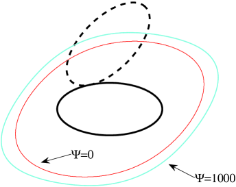
Figure 3: Line of $\Psi=0$ and $\Psi=1000$ for a pair of ellipses with aspect ratio $E=a/b=2$ with their axes rotated by 45^o for a function defined in Appendix B. Note that the thickness of the area between two lines of fixed $\Psi$ varies slightly.

In the numerical calculation of the stress, the limit in Eq. 26 is not easy to implement: Using a large $\Psi_{0}$ leads to an inaccurate answer, while using a small $\Psi_{0}$ leads to a small number of “almost contact” events, and, consequently, to large statistical errors. One may try considering a numerical extrapolation to $\Psi_{0}=0$ by measuring the stress for a sequence of decreasing $\Psi_{0}$s. However, the events for smaller values of $\Psi_{0}$ are also contained in set of the events for larger $\Psi_{0}$s. It is difficult to extrapolate such correlated sets of data points. The independence of the data points can be achieved by calculating a sequence of values of the stress for “contact shells” defined by $\Psi_{\alpha\beta}$ located in a sequence of segments $[0,\Psi_{0}),[\Psi_{0},2\Psi_{0}),\dots[K\Psi_{0},(K+1)\Psi_{0}),\dots$ ($K$ is integer). Values of $\sigma_{ij}$ now can be conveniently extrapolated to their “real” values. A similar method has been used by Farago and Kantor fk_formalism to calculate the stress and elastic constants of hard sphere solids.

The terms in the expressions for elastic constants including two pairs of particles can be similarly handled. One simply uses $\Psi_{01}$ and $\Psi_{02}$ to define two shells, $S(\Psi_{01})$ and $S(\Psi_{02})$, respectively, each corresponding to a particular contact, and considers the events which occur when both pairs of particles are within their respective shells simultaneously. E.g.,

$$\langle\Delta_{m}^{\alpha\beta}R^{\alpha\beta}_{n}\Delta_{i}^{\gamma\delta}R^{\gamma\delta}_{j}\rangle=$$

$$\lim_{{\Psi_{01}\to 0\atop\Psi_{02}\to 0}} \frac{1}{\Psi_{01}\Psi_{02}}\left\langle\frac{\partial\Psi^{\alpha\beta}}{\partial R^{\alpha\beta}_{m}}R^{\alpha\beta}_{n}\frac{\partial\Psi^{\gamma\delta}}{\partial R^{\gamma\delta}_{i}}R^{\gamma\delta}_{j}\right\rangle_{S(\Psi_{01}),S(\Psi_{02})}.$$ (27)

Compared with the case of the stress, the numerical evaluation of the limit where the thickness of the shells vanishes presents an even bigger numerical problem, since the probability of two contact events is very small. Nevertheless, this can be handled in a similar way, by considering a 2D array of segments of the type $\{[K\Psi_{0},(K+1)\Psi_{0}),[L\Psi_{0},(L+1)\Psi_{0})\}$ ($K$ and $L$ integers) and obtaining the values of the various parts of the elastic constants by extrapolating the 2D surface to its “real” value of vanishing contact layer thickness.

V Results of simulations

We used the method developed in this work to calculate the elastic properties of 2D hard ellipse system as a part of a study of its phase diagram mk . Here, we briefly demonstrate the usefulness of the method. As in any hard particle system, temperature plays no role, since the interactions have no “energy scale.” The temperature appears only as a multiplicative prefactor in the free energy $F$ and in Eq. 22 for the stress and Eq. 23 for the elastic constants. The results depend on the density of the particles and their size and shape: we characterized the system by the number of particles per unit area $\rho$ and by the sizes of the major and minor semi-axes, $a$ and $b$, of the ellipses. Frequently, reduced density $\rho^{*}\equiv 4\rho ab$ is used. The maximal possible (close packed) $\rho^{*}$ is independent of the aspect ratio $E=a/b$ of the ellipses and is equal to $2/\sqrt{3}\approx 1.155$. It should be noted vieillard that for every fixed $a$ and $b$ there is an infinity of possible (equally dense) close packed states which are obtained by orienting all ellipses in the same direction and packing them into a (distorted triangular) periodic structure.

The system of hard disks ($E=1$) has been extensively studied. For $\rho^{*}\gtrsim 0.91$ it forms a periodic 2D solid — a triangular lattice. The correlation function of atom positions of such a solid decays to zero as a power law of the separation between the atoms mermin . Such behavior is usually denoted as quasi-long-range order. At the same time the orientations of the “bonds” (imaginary lines connecting neighboring atoms) have a long range correlation mermin_bond . The system is liquid for $\rho^{*}\lesssim 0.89$, i.e it has no long range order of any kind. At the intermediate densities the system is probably hexatic hny — a phase with algebraically decaying bond-orientational order, but without positional order. (However, even very large scale simulations jm have difficulties in distinguishing the hexatic phase from coexisting solid and liquid phases.) From the point of view of elasticity theory, all three phases are isotropic, i.e. their second order elastic constants are determined by two independent constants. Aspect ratio $E\neq 1$ of the ellipses adds an additional order parameter — their orientation. E.g., for $E=4$ a system of ellipses forms isotropic liquid for densities $\rho^{*}\lesssim 0.8$. For larger densities the ellipses in the liquid become oriented (“nematic phase”). Finally, at $\rho^{*}\approx 1.0$ the system becomes a solid of orientationally ordered ellipses cuesta . For weakly elongated ellipses, we expect the particles to remain orientationally disordered in the entire liquid phase, and with increasing density to go (possibly via hexatic phase) to a crystalline state in which the ellipses remain disordered. The 3D analog of such a state is called plastic crystal plastic . (Presence of such a phase in almost circular ellipses ($E=1.01$) was observed by Vieillard-Baron vieillard .) With increasing density an additional phase transition will bring the ellipses into an orientationally ordered state. Phase diagram which includes such a transition between two solid phases for 3D hard ellipsoids has been studied by Frenkel et al. fmm .

As a test of our formalism we studied a case of moderately elongated hard ellipses with $E=1.5$. We considered system consisting of $N\approx 1000$ ellipses contained in a 2D rectangular box whose dimensions were chosen as close as possible to a square. Periodic boundary conditions were used. The ellipses were initially placed on a distorted triangular lattice, commensurate with the dimensions of a closed packed configuration corresponding to this particular aspect ratio $E$ and the particular orientation of the ellipses. In this Section we describe only the cases when the initial orientation of the major axes of the ellipses was taken to be perpendicular to one of the axes of symmetry of the ordered crystal drawn through neighboring particles. We first performed an equilibration run at constant pressure, in order to allow the system to reach an equilibrated state with respect to the orientational, as well as the translational ordering. The orientational order parameter, the box dimensions and the density were monitored during this equilibration run. A MC time unit in the equilibration run consisted of $N+1$ elementary moves, one of which, on the average, was a volume change attempt, and the rest were particle move attempts. A particle move attempt involved choosing a particle randomly, and attempting to displace and rotate it simultaneously by an amount chosen from a uniform distribution. The move was accepted if the displaced particle did not overlap in its new position and orientation with other particles. The volume change attempt was identical to that described in frenkel_bk . The width of the distributions corresponding to the particle moves and the parameter of the volume change were chosen so that the average success rates of both types of MC moves were about 50%.

The use of the constant pressure simulations at the equilibration stage enabled us to determine the equilibrium box shape for isotropic stress tensor (pressure) conditions. At most densities the final configuration had orientationally disordered ellipses, and we could easily verify that the final configurations were independent of the specific choice of the starting configuration. However, at extremely high densities, approaching the close packed density, even after long equilibration the state resembled the starting state of orientationally ordered ellipses. Typically, several millions of MC time units were required to reach equilibrium for a given pressure. Upon completion of equilibration, we switched to constant volume simulations, during which the stresses and the elastic constants were evaluated. Very long simulation times (about $10^{7}$ MC time units) were required for accurate determination of these constants, because their calculation depends on extremely rare events of two pairs of particles simultaneously touching each other. The range of “contact shells” was chosen in such a way that even in the most remote shell the separation between the particles was significantly smaller than their mean separation. The statistical accuracy of the elastic constants was evaluated by comparing the results of independent runs.

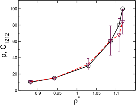
Figure 4: Pressure $p$ (open circles connected by solid line) and the elastic constant $C_{1212}$ (inverted open triangles connected by dashed line) of hard ellipse system with aspect ratio $E=1.5$ in the units of $kT/4ab$ as functions of the reduced density $\rho^{*}$. The error bars of the pressure are significantly smaller than the symbols denoting the data points.

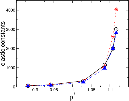
Figure 5: Elastic constants $C_{1111}$ (open circles connected by solid line), $C_{2222}$ (asterisks connected by dotted line) and $C_{1122}$ (full triangles connected by dot-dashed line) of hard ellipse system with aspect ratio $E=1.5$ in the units of $kT/4ab$ as functions of the reduced density $\rho^{*}$. The error bars of all the data points are slightly smaller than the symbols denoting them.

In a 2D system which has a reflection symmetry with respect to either $x$ or $y$ axis, the elastic constants with an index appearing an odd number of times (such as $C_{1112}$) must vanish. Indeed, our simulations showed that these quantities vanish within the error bars of the measurement. The system still may have four unrelated elastic constants $C_{1111}$, $C_{2222}$, $C_{1122}$ and $C_{1212}$. For a system with quadratic symmetry the number of independent elastic constants reduces to three. Such systems are frequently characterized by their bulk modulus and two shear moduli, $\mu_{1}=C_{1212}-p$ and $\mu_{2}=\frac{1}{2}(C_{1111}-C_{1122})-p$. For an isotropic system $\mu_{1}=\mu_{2}$ and, therefore, there are only two independent constants. (A system with six-fold symmetry is isotropic as far as the elastic constants are concerned.) Figs. 4 and 5 depict the pressure and four elastic constants for several values of the reduced density $\rho^{*}$. One can see that for densities $\rho^{*}\leq 1.086$, $C_{1111}$ and $C_{2222}$ practically coincide, indicating that these systems are at least quadratic. Furthermore, the identity $C_{1111}-C_{1122}=2C_{1212}$, i.e. $\mu_{1}=\mu_{2}$, is found to hold within a few percent for these values of $\rho^{*}$. Consequently, for these densities the system is isotropic from the point of view of the elastic properties. Figs. 6a, b and c depict the system in that range of densities: Figs. 6a and b represent states with vanishing shear moduli, and neither of them exhibits translational order of the ellipse centers. However, while Fig. 6a represents a state with all the characteristics of a liquid, the state in Fig. 6b is characterized by slowly decaying bond orientational order, possibly indicating hexatic phase. At a slightly higher density, Fig. 6c represents a plastic solid: while the ellipses are randomly oriented, the system exhibits long range bond orientational order, and algebraically decaying positional order of the particles. The particles occupy, on the average, positions of an undistorted triangular lattice although some undulations are apparent. This is characterized by two coinciding positive shear moduli.

When we approach within few percent the close packed configuration, corresponding to the two largest densities in Figs. 4 and 5 the prolonged relaxation process does not change the preferred orientation of the ellipses and the distortion of the lattice. It would be reasonable to conclude, that at such high density we finally arrived at the orientationally ordered elastic solid. The isotropic elastic symmetry no longer holds. We checked and found that almost all stability criteria birch ; zhou , indicating the sign of the energy change upon small deformation, are positive. However, one of the shear moduli, namely $\mu_{1}$, is slightly negative, although within one standard statistical deviation from zero. This, may either indicate that we are in an unstable state, or that there is a continuum of equilibrium states with different mean orientations of ellipses and, correspondingly, different dimensions of elementary cell.

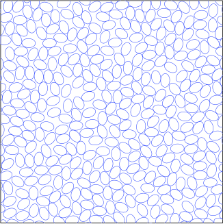
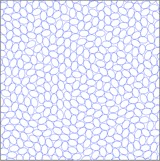
(a)                                                                     (b)

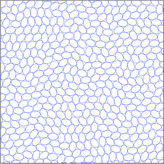
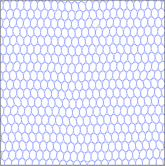
(c)                                                                     (d)

Figure 6: Typical equilibrium configurations of slightly eccentric ($E=1.5$) hard ellipse system at several densities. Only part of the system is shown. All the pictures show the same (partial) volume of the system; they differ only in the reduced density $\rho^{*}$: (a) orientationally and translationally disordered liquid at $\rho^{*}=0.881$; (b) liquid with a high degree of bond-orientational order at $\rho^{*}=1.029$; (c) plastic solid with long-range bond-orientational order, and quasi-long-range translational order consisting of rotationally disordered ellipses at $\rho^{*}=1.086$; (d) solid of orientationally ordered ellipses at $\rho^{*}=1.117$.

VI Discussion

We extended the formalism of SHH shh to the case of systems interacting via non-central two-particle potentials. In its form represented by Eqs. 15 and 16, the formalism can be used to study properties of molecular systems. This is particularly true for highly non-spherical organic molecules, and various soft condensed matter systems. The adaptation of the expressions to hard potentials (Eqs. 22 and 23) produced slightly more complicated expressions. However, the simplicity of hard potential systems provides excellent insights into the entropy-dominated systems. We demonstrated the usefulness of the formalism by presenting some results of our study of the hard ellipse system mk . Measurement of several order parameters, and the correlation functions is not always sufficient to determine the nature of phases. For systems of moderate size, it maybe even difficult to distinguish liquid from a solid. Measurement of elastic constants provides an additional, very important tool for assessing the nature of the state of the system. In particular, the elastic constants may indicate the presence of instability, even when prolonged equilibration does not change an existing state. Following the indications of instability at high densities, we are currently performing extensive study of equilibrium states at these densities.

While we worked on a 2D example, the method can be equally well applied in 3D for such systems as hard ellipsoids or spherocylinders.

Appendix A Regularization of diverging and poorly defined terms

Section III outlines the procedure for transition from expressions for soft potentials to expressions for hard potentials. The procedure relies on the fact, that despite the change in the potential between 0 and $\infty$, the expression for stress and some terms in the expression for for elastic constants contain a derivative of Boltzmann factor. Since the latter changes between 1 and 0, its derivatives involve $\delta$-function of the distance between the particles, leading to a finite thermal average. Even the terms containing contacts between two distinct pairs of particles, and, consequently, two $\delta$-functions of different variables, produce a finite results. However, the third line in Eq. 16 includes a term containing a product of two derivatives of the same pair of particles. A substitution of Eq. III into such an expression would lead to appearance of squared $\delta$-function and divergence of the entire term. Eq. 16 also contains second derivative of $\Phi$, which becomes poorly defined in the hard potential limit. Here we show that sum the two “problematic” terms described above has a well defined hard potential limit. Let us consider one particle pair $\langle\alpha\beta\rangle$:

$$\Bigg{\langle}\left(-\frac{1}{kT}\frac{\partial\Phi}{\partial R^{\alpha\beta}_{m}}\frac{\partial\Phi}{\partial R^{\alpha\beta}_{i}}+\frac{\partial^{2}\Phi}{\partial R^{\alpha\beta}_{m}\partial R^{\alpha\beta}_{i}}\right)R^{\alpha\beta}_{n}R^{\alpha\beta}_{j}\Bigg{\rangle}$$

$$=-kT\int d{\bf R}^{\alpha}d\Omega^{\alpha}\int d{\bf R}^{\beta}d\Omega^{\beta}\frac{\partial^{2}\ {\rm e}^{-\Phi({\bf R}^{\alpha\beta},\Omega^{\alpha},\Omega^{\beta})/kT}}{\partial R^{\alpha\beta}_{m}\partial R^{\alpha\beta}_{i}}R^{\alpha\beta}_{n}R^{\alpha\beta}_{j}P({\bf R}^{\alpha},\Omega^{\alpha},{\bf R}^{\beta},\Omega^{\beta})$$ (28)

In the internal integral in Eq. A we can replace $\partial/\partial R_{i}^{\alpha\beta}$ by $\partial/\partial R_{i}^{\beta}$, since the exponent only depends on ${\bf R}^{\beta}-{\bf R}^{\alpha}$. Following that, we perform integration by parts in which boundary term vanishes and arrive at

$$kT\int d{\bf R}^{\alpha}d\Omega^{\alpha}\int d{\bf R}^{\beta}d\Omega^{\beta}\frac{\partial\ {\rm e}^{-\Phi({\bf R}^{\alpha\beta},\Omega^{\alpha},\Omega^{\beta})/kT}}{\partial R^{\alpha\beta}_{m}}\frac{\partial}{\partial R^{\beta}_{i}}[R^{\alpha\beta}_{n}R^{\alpha\beta}_{j}P({\bf R}^{\alpha},\Omega^{\alpha},{\bf R}^{\beta},\Omega^{\beta})]$$

$$=-\int d{\bf R}^{\alpha}d\Omega^{\alpha}\int d{\bf R}^{\beta}d\Omega^{\beta}\frac{\partial\Phi}{\partial R^{\alpha\beta}_{m}}\ \ {\rm e}^{-\Phi({\bf R}^{\alpha\beta},\Omega^{\alpha},\Omega^{\beta})/kT}\left(\delta_{in}R^{\alpha\beta}_{j}P+\delta_{ij}R^{\alpha\beta}_{n}P+R^{\alpha\beta}_{n}R^{\alpha\beta}_{j}\frac{\partial P}{\partial R^{\beta}_{i}}\right).$$

The probability density $P$ in the above expressions was defined in Eq. III. Variable ${\bf R}^{\beta}$ appears in every potential that depends on some ${\bf R}^{\gamma\beta}$, and therefore, the derivative of $P$ with respect to $R^{\beta}_{i}$ in the last term of the above expression can be expressed in the following form:

$$\frac{\partial P}{\partial R^{\beta}_{i}}=\frac{1}{Z}\int\prod_{\lambda=1\atop\lambda\neq\alpha,\beta}^{N}(d{\bf R}^{\lambda}d\Omega^{\lambda})\frac{\partial}{\partial R^{\beta}_{i}}\ \ {\rm e}^{-\sum_{\langle\mu\nu\rangle\atop\neq\langle\alpha\beta\rangle}\Phi({\bf R}^{\mu\nu},\Omega^{\mu},\Omega^{\nu})/kT}$$ (30)

$$= \frac{1}{Z}\int\prod_{\lambda=1\atop\lambda\neq\alpha,\beta}^{N}(d{\bf R}^{\lambda}d\Omega^{\lambda})\sum_{\gamma\atop\neq\alpha,\beta}\frac{\partial}{\partial R^{\gamma\beta}_{i}}\ \ {\rm e}^{-\sum_{\langle\mu\nu\rangle\atop\neq\langle\alpha\beta\rangle}\Phi({\bf R}^{\mu\nu},\Omega^{\mu},\Omega^{\nu})/kT}$$

$$= -\frac{1}{kTZ}\int\prod_{\lambda=1\atop\lambda\neq\alpha,\beta}^{N}(d{\bf R}^{\lambda}d\Omega^{\lambda})\sum_{\gamma\atop\neq\alpha,\beta}\left[\frac{\partial\Phi}{\partial R^{\gamma\beta}_{i}}\right]\ \ {\rm e}^{-\sum_{\langle\mu\nu\rangle\atop\neq\langle\alpha\beta\rangle}\Phi({\bf R}^{\mu\nu},\Omega^{\mu},\Omega^{\nu})/kT}$$

Consequently, the term in Eq. A becomes:

$$-\left\langle\frac{\partial\Phi}{\partial R^{\alpha\beta}_{m}}R^{\alpha\beta}_{j}\delta_{in}+\frac{\partial\Phi}{\partial R^{\alpha\beta}_{m}}R^{\alpha\beta}_{n}\delta_{ij}\right\rangle+\frac{1}{kT}\sum_{\gamma\atop\neq\alpha,\beta}\left\langle\frac{\partial\Phi}{\partial R^{\alpha\beta}_{m}}\frac{\partial\Phi}{\partial R^{\gamma\beta}_{i}}R^{\alpha\beta}_{n}R^{\alpha\beta}_{j}\right\rangle$$ (31)

(This answer is slightly non-symmetric — this reflects the fact that we manipulated the integral over the variable ${\bf R}^{\beta}$, rather that ${\bf R}^{\alpha}$. In the latter case instead of partial derivative with respect to $R^{\gamma\beta}_{i}$ we would have obtained a partial derivative with respect to $R^{\alpha\gamma}_{m}$. ) When this result is substituted in the expression for the elastic constants in Eq. 16 we get

$$V_{0}C_{ijmn} = NkT(\delta_{im}\delta_{jn}+\delta_{in}\delta_{jm})$$ (32)

$$+ \frac{1}{4kT}\sum_{\langle\alpha\beta\rangle}\left\langle\frac{\partial\Phi}{\partial R^{\alpha\beta}_{i}}R^{\alpha\beta}_{j}+\frac{\partial\Phi}{\partial R^{\alpha\beta}_{j}}R^{\alpha\beta}_{i}\right\rangle\sum_{\langle\gamma\delta\rangle}\left\langle\frac{\partial\Phi}{\partial R^{\gamma\delta}_{m}}R^{\gamma\delta}_{n}+\frac{\partial\Phi}{\partial R^{\gamma\delta}_{n}}R^{\gamma\delta}_{m}\right\rangle$$

$$- \frac{1}{4kT}\sum_{\langle\alpha\beta\rangle}\sum_{\langle\gamma\delta\rangle\atop\neq\langle\alpha\beta\rangle}\Bigg{\langle}\frac{\partial\Phi}{\partial R^{\alpha\beta}_{m}}\frac{\partial\Phi}{\partial R^{\gamma\delta}_{i}}R^{\alpha\beta}_{n}R^{\gamma\delta}_{j}+\frac{\partial\Phi}{\partial R^{\alpha\beta}_{n}}\frac{\partial\Phi}{\partial R^{\gamma\delta}_{i}}R^{\alpha\beta}_{m}R^{\gamma\delta}_{j}$$

$$+ \frac{\partial\Phi}{\partial R^{\alpha\beta}_{m}}\frac{\partial\Phi}{\partial R^{\gamma\delta}_{j}}R^{\alpha\beta}_{n}R^{\gamma\delta}_{i}+\frac{\partial\Phi}{\partial R^{\alpha\beta}_{n}}\frac{\partial\Phi}{\partial R^{\gamma\delta}_{j}}R^{\alpha\beta}_{m}R^{\gamma\delta}_{i}\Bigg{\rangle}$$

$$+ \frac{1}{8kT}\sum_{\langle\alpha\beta\rangle}\sum_{\gamma\atop\neq\alpha,\beta}\Bigg{\langle}\frac{\partial\Phi}{\partial R^{\alpha\beta}_{m}}\left(\frac{\partial\Phi}{\partial R^{\gamma\beta}_{i}}+\frac{\partial\Phi}{\partial R^{\alpha\gamma}_{i}}\right)R^{\alpha\beta}_{n}R^{\alpha\beta}_{j}+\frac{\partial\Phi}{\partial R^{\alpha\beta}_{n}}\left(\frac{\partial\Phi}{\partial R^{\gamma\beta}_{i}}+\frac{\partial\Phi}{\partial R^{\alpha\gamma}_{i}}\right)R^{\alpha\beta}_{m}R^{\alpha\beta}_{j}$$

$$+ \frac{\partial\Phi}{\partial R^{\alpha\beta}_{m}}\left(\frac{\partial\Phi}{\partial R^{\gamma\beta}_{j}}+\frac{\partial\Phi}{\partial R^{\alpha\gamma}_{j}}\right)R^{\alpha\beta}_{n}R^{\alpha\beta}_{i}+\frac{\partial\Phi}{\partial R^{\alpha\beta}_{n}}\left(\frac{\partial\Phi}{\partial R^{\gamma\beta}_{j}}+\frac{\partial\Phi}{\partial R^{\alpha\gamma}_{j}}\right)R^{\alpha\beta}_{m}R^{\alpha\beta}_{i}\Bigg{\rangle}$$

$$- \frac{1}{4}\sum_{\langle\alpha\beta\rangle}\Bigg{\{}\left\langle\frac{\partial\Phi}{\partial R^{\alpha\beta}_{j}}R^{\alpha\beta}_{n}+\frac{\partial\Phi}{\partial R^{\alpha\beta}_{n}}R^{\alpha\beta}_{j}\right\rangle\delta_{im}+\left\langle\frac{\partial\Phi}{\partial R^{\alpha\beta}_{i}}R^{\alpha\beta}_{m}+\frac{\partial\Phi}{\partial R^{\alpha\beta}_{m}}R^{\alpha\beta}_{i}\right\rangle\delta_{jn}$$

$$+ \left\langle\frac{\partial\Phi}{\partial R^{\alpha\beta}_{i}}R^{\alpha\beta}_{n}+\frac{\partial\Phi}{\partial R^{\alpha\beta}_{n}}R^{\alpha\beta}_{i}\right\rangle\delta_{jm}+\left\langle\frac{\partial\Phi}{\partial R^{\alpha\beta}_{j}}R^{\alpha\beta}_{m}+\frac{\partial\Phi}{\partial R^{\alpha\beta}_{m}}R^{\alpha\beta}_{j}\right\rangle\delta_{in}$$

$$+ \left\langle\frac{\partial\Phi}{\partial R^{\alpha\beta}_{m}}R^{\alpha\beta}_{n}+\frac{\partial\Phi}{\partial R^{\alpha\beta}_{n}}R^{\alpha\beta}_{m}\right\rangle\delta_{ij}+\left\langle\frac{\partial\Phi}{\partial R^{\alpha\beta}_{i}}R^{\alpha\beta}_{j}+\frac{\partial\Phi}{\partial R^{\alpha\beta}_{j}}R^{\alpha\beta}_{i}\right\rangle\delta_{mn}\Bigg{\}}.$$

Since the above expressions contain only the first derivatives of the potentials (or products of such terms for non-identical pairs of particles) we can use Eqs. III and 21 to calculate the elastic constants for hard potentials.

Appendix B Overlap function of two ellipses

A crucial difficulty in the simulations of hard ellipses in 2D and hard spheroids in 3D is the determination whether two such objects overlap. Vieillard-Baron derived a contact function for the 2D case of ellipses vieillard . His function enables a reasonably fast determination of the presence of an overlap. It can also be used to determine the direction of the inter-ellipse force and, consequently, can be used in determination of stresses and elastic constants. In this Appendix we describe this function and its properties.

Consider two identical ellipses, $\alpha$ and $\beta$, whose major and minor semi-axes are $a$ and $b$, respectively. Let their centers be separated by vector ${\bf R}^{\alpha\beta}$, and one of them be rotated compared to the other one by the angle $\theta$. Projections of ${\bf R}^{\alpha\beta}$ on the directions of major and minor semi-axes of ellipse $\alpha$ will be denoted $R^{\alpha\beta}_{\alpha 1}$ and $R^{\alpha\beta}_{\alpha 2}$, respectively. Then we can define a contact function

$$\Psi^{\alpha\beta}=4(h_{\alpha}^{2}-3h_{\beta})(h_{\beta}^{2}-3h_{\alpha})-(9-h_{\alpha}h_{\beta})^{2},$$ (33)

where for each ellipse we define

$$h_{\alpha}=1+G-[(R^{\alpha\beta}_{\alpha 1}/a)^{2}+(R^{\alpha\beta}_{\alpha 2}/b)^{2}],$$ (34)

and

$$G=2+\left(\frac{a}{b}-\frac{b}{a}\right)^{2}\sin^{2}\theta.$$ (35)

Function $\Psi^{\alpha\beta}$ depends on the distance between the ellipses and on their orientation. The number of overlap points of two ellipses can vary between 0 and 4. The necessary and sufficient condition for ellipses to have no intersection points is $\Psi^{\alpha\beta}>0$ and at least one of the two functions $h_{\alpha}$ and $h_{\beta}$ be negative. The proof of this statement can be found in Ref. vieillard . At the contact $\Psi^{\alpha\beta}=0$. In the region where the ellipses do not intersect the function $\Psi^{\alpha\beta}$ has no extremum points; thus if $\Psi^{\alpha\beta}$ is sufficiently small, i.e. $0\leq\Psi^{\alpha\beta}<\Psi_{0}$ we can be assured that two ellipses are close to each other.

When the ellipses degenerate into a circles, i.e. $a=b$, the contact function becomes only a function of the distance between the centers of the circles $R^{\alpha\beta}$

$$\Psi^{\alpha\beta}=3\left(\frac{R^{\alpha\beta}}{a}\right)^{6}\left[\left(\frac{R^{\alpha\beta}}{a}\right)^{2}-4\right].$$ (36)

Note, that the gradient of this function at the distance of contact between the circles has a rather large value $768/a$, so even if we choose $\Psi^{\alpha\beta}=8$ the circles will be about 1% of the radius away from each other.

The shell between the lines $\Psi^{\alpha\beta}=0$ and $\Psi^{\alpha\beta}=\Psi_{0}$ has a uniform thickness for circles, but its thickness varies with position in ellipses as can be seen in the Fig. 3. When the aspect ratio of the ellipse becomes much larger than unity the thickness becomes strongly variable which will adversely influence the accuracy of Monte Carlo simulations.

References

- (1) L. D. Landau and E. M. Lifshits, Theory of Elasticity (Pergamon Press, Oxford, 1986).
- (2) T. H. K. Barron and M. L. Klein, Proc. Phys. Soc. 85, 523 (1965).
- (3) Z. Hashin, Theory of Fiber Reinforced Materials, pp.44-47 (NASA, Langley Research Center, Hampton, Virginia, 1970).
- (4) F. Birch, Phys. Rev. 71, 809 (1947).
- (5) Z. Zhou and B. Joós, Phys. Rev. B 54, 3841 (1996).
- (6) D. R. Squire, A. C. Holt and W. G. Hoover, Physica 42, 388 (1969).
- (7) M. Born and K. Huang, Dynamical Theory of Crystal Lattices (Oxford University Press, Oxford, 1954), p. 129.
- (8) R. K. Pathria, Statistical Mechanics, 2nd ed. (Butterworth-Heinemann, Oxford, 1996); M. Toda, R. Kubo, and N. Saito, Statistical Physics: Equilibrium Statistical Mechanics Part I (Springer, Berlin, 1998); R. Balescu, Equilibrium and Nonequilibrium Statistical Mechanics (Wiley, NY, 1975).
- (9) O. Farago and P. Pincus, J. Chem. Phys. 120, 2934 (2004).
- (10) M. Parrinello and A. Rahman, J. Chem. Phys. 76, 2662 (1982); See also, A. A. Gusev, M. M. Zehnder and U. W. Suter, Phys. Rev. B 54, 1 (1996), and references therein.
- (11) F. Bavaud, Ph. Choquard, and J.-R. Fontaine, J. Stat. Phys. 42, 621 (1986).
- (12) N. Metropolis, A. W. Rosenbluth, M. N. Rosenbluth, A. H. Teller and E. Teller, J. Chem. Phys. 21, 1087 (1953).
- (13) A. P. Gast and W. B. Russel, Phys. Today 51, 24 (1998).
- (14) W. G. Hoover and F. H. Ree, J. Chem. Phys. 49, 3609 (1968), and 47, 4873 (1967); B. J. Alder, W. G. Hoover, and D. A. Young, J. Chem. Phys. 49, 3688 (1968).
- (15) D. Frenkel and A. J. C. Ladd, Phys. Rev. Lett. 59, 1169 (1987).
- (16) K. J. Runge and G. V. Chester, Phys. Rev. A 36, 4852 (1987).
- (17) H. M. James and E. Guth, J. Chem. Phys. 11, 455 (1943). P. J. Flory, J. Am. Chem. Soc. 63, 3083 (1941).
- (18) P. G. de Gennes, Scaling Concepts in Polymer Physics (Cornell University Press, Ithaca, N.Y., 1979).
- (19) S. Panyukov and Y. Rabin, Phys. Rep. 269, 1 (1996); H. E. Castillo and P. M. Goldbart, Phys. Rev. E 58, R24 (1998); P. M. Goldbart, H.C. Castillo and A. Zippelius, Adv. Phys. 45, 393 (1996).
- (20) A. Baumgärtner, p. 145 in Application of the Monte Carlo Method in Statistical Physics (Topics in Current Physics, vol. 36), ed. by K. Binder, 2nd ed., (Springer, Berlin, 1987).
- (21) Y. Kantor, M. Kardar and D. R. Nelson, Phys. Rev. Lett. 57, 791 (1986); and Phys. Rev. A 35, 3056 (1987).
- (22) O. Farago and Y. Kantor, Phys. Rev. E 61, 2478, 2000.
- (23) O. Farago and Y. Kantor, Phys. Rev. Lett. 85, 2533, 2000.
- (24) O. Farago and Y. Kantor, Europhys. Lett. 57, 458, 2002.
- (25) O. Farago and Y. Kantor, The European Phys. J. E 3, 253, 2000, and Europhys. Lett. 52, 413, 2000.
- (26) P. G. de Gennes and J. Prost, The Physics of Liquid Crystals, 2nd ed. (Oxford University Press, 1995).
- (27) L. Onsager, Ann. NY Acad. Sci. 51, 627 (1949).
- (28) D. Frenkel and R. Eppenga, Phys. Rev. Lett. 49, 1089 (1982); R. Eppenga and D. Frenkel, Mol. Phys. 52, 1303 (1984); M. A. Bates and D. Frenkel, Phys. Rev. E 57, 4824 (1998).
- (29) D. Frenkel and J. F. Maguire, Mol. Phys. 49, 503 (1983), and Phys. Rev. Lett. 47, 1025 (1981).
- (30) D. Frenkel, B. M. Mulder, and J. P. McTague, Phys. Rev. Lett. 52, 287 (1984).
- (31) Th. Theenhaus, M. P. Allen, M. Letz, A. Latz, and R. Schilling, Eur. Phys. J. E 8, 269 (2002); U. P. Singh and Y. Singh, Phys. Rev. A 33, 2725 (1986); M. Baus, J.-L. Colot, X.-G. Wu, and H. Xu, Phys. Rev. Lett. 59, 2184 (1987).
- (32) D. Frenkel, H. N. W. Lekkerkerker, and A. Stroobants, Nature (London) 332, 822 (1988); E. Velasco, L. Mederos, D. E. Sullivan, Phys. Rev. E 62, 3708 (2000); A. Poniewierski and R. Holyst, Phys. Rev. Lett. 61, 2461 (1988). S. C. McGrother, D. C. Williamson, and G. Jackson, J. Chem. Phys. 104, 6755 (1996); J. M. Polson and D. Frenkel, Phys. Rev. E 56, R6260 (1997); P. Bolhuid and D. Frenkel, J. Chem. Phys. 106, 666 (1997).
- (33) F. Schmid and N. H. Phuong, cond-mat/0208448 (2002).
- (34) K. W. Wojciechowski, K. V. Tretiakov, and M. Kowalik, Phys. Rev. E 67, 036121 (2003).
- (35) D. C. Williamson and G. Jackson, J. Chem. Phys. 108, 10284 (1998); K. W. Wojciechowski, Phys. Rev. B 46, 26 (1992); C. McBride, C. Vega, and L. G. MacDowell, Phys. Rev. E, 64, 011703 (2001).
- (36) D. C . Williamson and F. del Rio, J. Chem. Phys. 109, 4675 (1998); Z. Varga and I. N. Szalai, Mol. Phys. 95, 515 (1998).
- (37) J. Vieillard-Baron, J. Chem. Phys. 56, 4729 (1972).
- (38) J. A. Barker and D. Henderson, Mol. Phys. 21, 187 1971
- (39) M. P. Alen, G. T. Evans, D. Frenkel, B. M. Mulder, Adv. Chem. Phys. 86, 1 (1993).
- (40) W. G. Hoover, Computational Statistical Mechanics, (Elsevier, 1991).
- (41) D. Frenkel and B. Smit, Understanding Molecular Simulation. From Algorithm to Applications, 2nd ed. (Academic Press, Boston, 2002).
- (42) K. Binder and D. W. Heermann, Monte Carlo Simulation in Statistical Physics (Springer, Berlin, 1997).
- (43) J. W. Perram, M. S. Wertheim, J. L. Lebowitz, and G. O. Williams, Chem. Phys. Lett. 105, 277 (1984); J. W. Perram and M. S. Wertheim, J. Computational Phys. 58, 409 (1985).
- (44) J. W. Perram, J. Rasmussen, E. Præstgaard, and J. L. Lebowitz, Phys. Rev. E 54, 6565 (1996).
- (45) M. Murat and Y. Kantor, to be published.
- (46) N. D. Mermin and H. Wagner, Phys. Rev. Lett. 17, 1133 (1966).
- (47) N. D. Mermin, Phys. Rev. 176, 250 (1968).
- (48) B. I. Halperin and D. R. Nelson, Phys. Rev. Lett. 41, 121 (1978); D. R. Nelson and B. I. Halperin, Phys. Rev. B 19, 2457 (1979); A. P. Young, Phys. Rev. B 19, 1855 (1979).
- (49) A. Jaster, Phys. Lett. A 330, 120 (2004); C. H. Mak, cond-mat/0502216 (2005), and references therein.
- (50) J. A. Cuesta and D. Frenkel, Phys. Rev. A 42, 2126 (1990).
- (51) D. Fox, M. M. Labes and A. Weissberger, editors, Physics and Chemistry of Organic Solid State, vol. 1 (Interscience, New York, 1963).