Quantum-based Mechanical Force Realization in Pico-Newton Range

Abstract

We propose mechanical force realization based on flux quantization in the pico-Newton range. By controlling the number of flux quantum in a superconducting annulus, a force can be created as integer multiples of a constant step. For a 50 nm-thick Nb annulus with the inner and outer radii of 5 $\mu$m and 10 $\mu$m, respectively, and the field gradient of 10 T/m the force step is estimated to be 184 fN. The stability against thermal fluctuations is also addressed.

Introduction

Due to remarkable improvement in its sensitivity, force measurement has become a useful and essential probe for leading-edge nano/bio-researchesPratt04 , which cover nanoscale imaging, protein folding studies, nanoindentation, and many others. The force detection limit keeps getting lowered, for example, to an atto-Newton (10^-18 N) level in magnetic resonance force microscopy. Such an ultimate resolution is enough to read a single electron spin.Rugar04 ; Knobel03a ; Huang03a

Unfortunately, however, no direct SI-traceable force realization has been established even at sub-Newton level, which means no standard to compare with measured force. Prevailing dead-weight method, which creates gravitational force using standard weights, obviously becomes no longer valid below micro-Newton level.Pratt04 At the micro-Newton level, an electrostatic force realization has been proposed recently by Pratt et al. Therein, electrostatic standard force is created between two coaxial electrodes in maintaining a constant voltage and expected to allow a relative uncertainty of parts in $10^{4}$. Related electrical units are traced to their standards based on Josephson and quantized Hall effects. At the nano-Newton or pico-Newton level, no force realization for standard has been suggested despite needs for precision measurements of force. It is essential, for instance, to testify fundamental forces such as Casimir force, non-Newtonian gravitation,Chiave03 etc.

Also, it casts a striking contrast to the case of electrical units such as voltage, that (to our best knowledge) no attempt has been tried to directly use quantum phenomena in realizing a mechanical force. Here, we present a concept of quantum-based force realization utilizing a macroscopic quantum phenomenon known as magnetic flux quantization in a superconducting annulus. Magnetic force exerted on flux quanta can be increased or decreased by a constant step, which is estimated to be sub-pico-Newton level. Moreover, those force-generating states are stable and robust against thermal fluctuation at liquid helium temperature.

Basic Principles

Figure 1 shows a schematic of quantum-based force realization. A tens-micron-sized superconducting annulus is mounted on an ultrasoft micro-cantilever. Below a superconducting transition temperature of the superconducting material, magnetic fluxoid through the annulus is quantized, and the resultant magnetic moment has a component with constant steps, the number of which depends on the quantum number. The step size is determined by fundamental constants such as electron charge and the length quantities of the annulus.

In a calibrated magnetic field gradient, dB/dz, a force is created on the superconducting annulus, and therefore on the micro-cantilever. Through a designed procedure of magnetic field and temperature, we can leave trapped flux quanta as many as we want in zero external field, while the field gradient is not zero. The displacement of the cantilever is monitored by optic interferometer or lever and can be used in calibrating its spring constant.

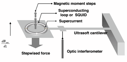
Figure 1: A schematic of force realization based on flux quantization in superconducting annulus.

Magnetic Moment of a Superconducting Annulus

For the accurate force realization, it is essential first to evaluate the magnetic moment of the superconducting annulus.

We consider a superconducting annulus of inner and outer radii, $a$ and $b$, respectively, and thickness $d$ in a uniform external magnetic field $\mathbf{B}_{\mathrm{ext}}=B_{\mathrm{ext}}\hat{\mathbf{z}}$. In response to the external magnetic field or the fluxoid trapped in the hole, currents $\mathbf{J}$ are induced in the annulus and the field is modified. The net magnetic vector potential $\mathbf{A}=\mathbf{A}_{\mathrm{ext}}+\mathbf{A}_{\mathrm{ind}}$ consists of the external part $\mathbf{A}_{\mathrm{ext}}$ and the induced part $\mathbf{A}_{\mathrm{ind}}$. $\mathbf{J}$ and $\mathbf{A}_{\mathrm{ind}}$ are related the Biot-Savart law

$$\mathbf{A}_{\mathrm{ind}}(\mathbf{r})=\int{d^{3}\mathbf{r}^{\prime}}\frac{\mu_{0}\mathbf{J}(r^{\prime})}{4\pi|\mathbf{r}-\mathbf{r}^{\prime}|}\,,$$ (1)

where $\mu_{0}$ is the magnetic permeability. On the other hand, within a superconductor, the current is governed by the London equation

$$\mathbf{J}=-\frac{1}{\mu_{0}\lambda_{L}^{2}}\left(\mathbf{A}+\frac{\Phi_{0}}{2\pi}\boldsymbol{\nabla}\theta\right)\,,$$ (2)

where $\theta$ is the phase of the superconducting order parameter, $\lambda_{L}$ is the London penetration depth, and $\Phi_{0}\equiv{h}/2|e|\approx 2.07\times 10^{-15}\mathrm{weber}$ is the flux quantum. Equations (1) and (2) give an integral equation for $\mathbf{J}$, from which one can get the magnetic moment. Given the geometry of the superconductor, one can greatly simplify the integral equation by following Brandt04a .

Since the current flows only in the thin film ($-d/2\leq z\leq d/2$, $d\ll\lambda_{L}$), it is customary to define a sheet current such that $\mathbf{J}(x,y,z)\approx\mathbf{J}_{\mathrm{sheet}}(x,y)\delta(z)$ and to represent the physical quantities in the polar coordinates $(r,\varphi,z)$ so that $\mathbf{J}_{\mathrm{sheet}}(x,y)=\mathbf{J}_{\mathrm{sheet}}(r)\hat{\varphi}$, $\mathbf{A}(x,y,0)=[A_{\mathrm{ext}}(r)+A_{\mathrm{ind}}(r)]\hat{\varphi}$, and $\boldsymbol{\nabla}\theta(x,y,0)=(n/r)\hat{\varphi}$, where the integer $n$ is the number of fluxes trapped in the hole. Then the London equation (2) reads as

$$\mu_{0}J_{\mathrm{sheet}}(r)=-\frac{1}{\Lambda}\left[\frac{n\Phi_{0}}{2\pi r}+A_{\mathrm{ext}}(r)+A_{\mathrm{ind}}(r)\right]$$ (3)

where $\Lambda\equiv\lambda_{L}^{2}/d$ is the effective penetration depth and the Biot-Savart law (1) is rewritten as

$$A_{\mathrm{ind}}(r)=\int_{a}^{b}{dr^{\prime}}Q(r,r^{\prime})\,\mu_{0}J_{\mathrm{sheet}}(r^{\prime})\,,$$ (4)

where

$$Q(r,r^{\prime})=\int_{0}^{\pi}\frac{d\varphi}{2\pi}\;\frac{\cos\varphi}{\sqrt{1-2(r/r^{\prime})\cos\varphi+(r/r^{\prime})^{2}}}\,.$$ (5)

From the London equation (3), one identifies two sources: one from the London fluxoid London54a $D_{1}(r)\equiv{n\Phi_{0}}/{2\pi r}$ and the other from the external field $D_{2}(r)\equiv A_{\mathrm{ext}}(r)$. Accordingly, we decompose the induced quantities, $J_{\mathrm{sheet}}$ and $A_{\mathrm{ind}}$, into contributions from $D_{1}$ and $D_{2}$, respectively: $J_{\mathrm{sheet}}=J_{1}+J_{2}$ and $A_{\mathrm{ind}}=A_{1}+A_{2}$. Combining the two equations (3) and (4), one arrives at the integral equations for $J_{1}$ and $J_{2}$

$$\int_{a}^{b}{dr^{\prime}}\;Q(r,r^{\prime})\,\mu_{0}J_{\nu}(r^{\prime})+\Lambda\,\mu_{0}J_{\nu}(r)=-D_{\nu}(r),$$ (6)

respectively ($\nu=1,2$)Brandt04a ; Fetter80b . The nice feature of this form is that $a\leq r\leq b$, which facilitates pretty much the numerical solution of the equation. Once $J_{\nu}$ ($\nu=1,2$) are at hand, the magnetic moment $m=m_{1}+m_{2}$ is given by

$$m_{\nu}=\pi\int_{a}^{b}{dr}\;r^{2}J_{\nu}(r)\,.$$ (7)

We have followed Brandt04a to discretize the integral equation (6) and get $J_{\nu}$ and $m_{\nu}$ numerically.

Figure 2 shows typical behavior of the total magnetic moment $m$ of the superconducting annulus as a function of $B_{\mathrm{ext}}$. It is clearly seen that at a given $B_{\mathrm{ext}}$, the magnetic moment is quantized depending on the number of trapped fluxes.

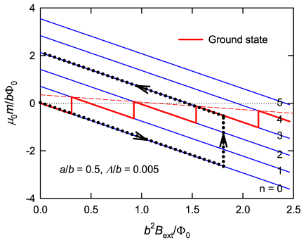
Figure 2: (color online) Total magnetic moment as a function of $B_{\mathrm{ext}}$ for $n$ trapped fluxoids (solid blue lines), $a/b=0.5$, and $\Lambda/b=0.005$. The thick (red) line is for the ground state configuration. The dashed (red) line is the guide for eyes connecting the peaks of ground-state magnetic moment. The thick dotted (black) line indicates the experimental procedure (see the text).

At a given value of $B_{\mathrm{ext}}$, the allowed quantized value of the magnetic moment corresponds to a metastable state of the system (the thin blue lines in Fig. 2). The magnetic moment corresponding to the most stable state (the thick red line in Fig. 2) is determined by the Gibbs free energy Brandt04a

$$G_{n}(B_{\mathrm{ext}})=-\frac{1}{2}mB_{\mathrm{ext}}+\frac{1}{2}n\Phi_{0}I\,,$$ (8)

where $I=I_{1}+I_{2}$ with $I_{\nu}=\int_{a}^{b}{dr}\;J_{\nu}(r)$ is the total current along the annulus. The ground-state magnetic moment is a periodic function of $B_{\mathrm{ext}}$ with period $B_{0}$. Figure 3 plots $B_{0}$ versus $a/b$.

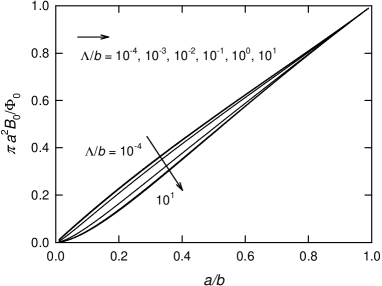
Figure 3: $B_{0}$ as a function of $a/b$ for different values of $\Lambda/b$.

Estimation of Magnetic Moment, Force Step, Force Limit

To estimate the magnitude of the magnetic moment, let us consider an Nb annulus of inner and outer radii, $a=5$ $\mu$m and $b=10$ $\mu$m, respectively, with thickness of 50 nm. The Nb material was chosen because its superconducting transition temperature, 9.25 K,Pool00 is readily accessible in cryogenics and its thin film fabrication is well established to have provided good quality of thin-film circuits such as SQUID. Its London penetration depth $\lambda_{L}$ and coherence length $\xi$ are 50 nm and 39 nm, respectively.Pool00 The choice of radii is reasonable considering the typical dimension of microfabricated cantilevers with a low spring constant ($k=10^{-4}$ to $10^{-5}$ N/m).Mamin01 These parameters fall on the case of $a/b=0.5$ and $\Lambda/b=0.005$.

Then, a magnetic moment step, $m_{Q}$, by adding a single flux quantum, is numerically estimated as 1.116 $m_{b}$, where the magnetic moment unit $m_{b}\equiv\Phi_{0}b/\mu_{0}$ is $1.65\times 10^{-14}\mathrm{A\cdot m^{2}}$. The force on the superconducting annulus is given by

$$F=m_{Q}\frac{dB_{ext}}{dz}\,$$ (9)

and assuming a modest field gradient, $dB_{ext}/dz$, of 10 T/m,Gradient a corresponding force step is estimated to be $1.84\times 10^{-13}$ N or 184 fN, which causes $\sim 2$ nm static displacement of a cantilever with $k=10^{-4}$ N/m. In principle, nano- and pico-Newton level can be accessed by stacking these steps.

Practically, a maximum possible force, or the maximum number of steps, is limited by the critical current of the superconducting material, at which its superconducting state cannot be sustained. For the Nb annulus with above geometry, the force limit is roughly estimated to be $\sim$ 40 pN from the approximate equation $F_{max}=I_{c}\pi[(a+b)/2]^{2}(dB/dz)$ and the critical current density of Nb, $j_{c}=9\times 10^{10}$ A/m² at $T=$ 6 K.Geers01

Force Realization Procedure

Realization of only a quantum-induced force requires a specially designed procedure, because the magnetic moment of a superconducting annulus includes a field-induced component linearly proportional $B_{ext}$ as seen in Fig. 2. The magnetic field at the annulus from the z-gradient magnet, the background, and so on is not simple to null satisfactorily, considering the small value of $B_{0}$ ($\sim$ 0.13 Oe for the parameters above), and would generate a non-zero force offset even in zero flux quantum state. Therefore, we need to extract selectively the flux quantum contribution.

In Fig. 2, the difference of magnetic moment, for example, between $n=0$ and $n=3$ states is always constant, three-times as large as $m_{Q}$ at any fixed $B_{ext}$, and a corresponding change can be realized by transition between them in principle. Uncontrolled transitons, such as quantum or thermal tunneling (to be discussed later), are practically negligible at operation temperatures, $\sim 4$ K, due to high energy barriers between metastable states.

We suggest a force-realization and cantilever-calibration procedure as follows: (1) After measuring a zero-reference position of a cantilever in $n=n_{i}$ state at $B_{ext}=0$ and $T\ll T_{c}$, turn on a uniform external field up to a target value roughly where $n=n_{f}=n_{i}+\Delta n$ is a global minimum of Gibbs free energy. But, the system still stays at $n=n_{i}$ state due to energy barriers. (2) Then, increase temperature above $T_{c}$ and decrease it back to $T\ll T_{c}$, which would send the system to the global minimum state, $n=n_{f}$. (3) Decrease and turn off the uniform external field and measure the displacement of the cantilever. The net change of magnetic moment, $\Delta n\times m_{Q}$, is only related to flux quanta and so is that of a force. From the number change of flux quantum ($\Delta n$), annulus dimension, penetration depth, and field gradient, the change in force can be evaluated and used in determining the spring constant of the cantilever in combination with its displacement.

The starting condition $B_{ext}=0$ can be lifted; our procedure is still valid even for $B_{ext}\neq 0$ as long as it is the same at the beginning and the end. This is a great benefit because background magnetic field is hard to shield and usually disturbs delicate magnetic experiments.

In-Situ Calibration of Field Gradient

For precise force realization, one has to be able to calibrate the magnetic field gradient $dB_{\mathrm{ext}}/dz$ as accurate as possible. Experimentally, it is tricky to know the exact value at the local position of the annulus on a micro-cantilever, unless the field gradient is strictly uniform in a large volume and well pre-calibrated in micro-scale.

Here we argue that we can calibrate it in-situ by means of the characteristic properties of the magnetic moment of the superconducting annulus. The magnetization $m(B_{\mathrm{ext}})$ in Eq. (9) can be written into the form

$$m=m_{1}(n)+\chi B_{\mathrm{ext}}\,,\quad\chi\equiv\frac{m_{2}(B_{\mathrm{ext}})}{B_{\mathrm{ext}}}\,,$$ (10)

where it should be noticed that $m_{1}(n)$ and $m_{2}(B_{\mathrm{ext}})$ are linearly proportional to $n$ and $B_{\mathrm{ext}}$, respectively. The field is expanded as

$$B_{\mathrm{ext}}(z)=B_{\mathrm{ext},0}+\frac{dB_{\mathrm{ext}}}{dz}z\,.$$ (11)

From Eqs. (9), (10), and (11), the force $F(z)$ at the position $z$ is given by

$$F(z)=\left[m_{1}(1)n+\chi B_{\mathrm{ext},0}\right]\frac{dB_{\mathrm{ext}}}{dz}+\chi\left(\frac{dB_{\mathrm{ext}}}{dz}\right)^{2}z\,.$$ (12)

Then it follows that

$$\frac{\Delta\omega}{\omega}=\frac{1}{2}\frac{\Delta k}{k}=\frac{\chi}{2k}\left(\frac{dB_{\mathrm{ext}}}{dz}\right)^{2}\,,$$ (13)

where $w$ ($k$) is the natural vibration frequency (Hook’s coefficient) of the cantilever and $\Delta{w}$ ($\Delta{k}$) is the shift in $w$ ($k$) due to the field gradient. Let $\Delta{z}=z_{\mathrm{eq}}(n)-z_{\mathrm{eq}}(n=0)$, i.e., the shift in the equilibrium position $z_{\mathrm{eq}}$ for non-zero flux $n$. Since the force $F(z_{\mathrm{eq}})$ at $z=z_{\mathrm{eq}}$ in Eq. (12) should be at equilibrium with $(k+\Delta k)z_{\mathrm{eq}}$, i.e.,

$$m_{1}(1)n\frac{dB_{\mathrm{ext}}}{dz}=k\Delta z\,,$$ (14)

one arrives at the relation

$$\frac{dB_{\mathrm{ext}}}{dz}=\frac{2n}{\Delta z}\frac{m_{1}(1)}{\chi}\frac{\Delta\omega}{\omega}\,.$$ (15)

We now note that in Eq. (15), the field gradient $dB_{\mathrm{ext}}/dz$ has been expressed only in known quantities of quantities that can be determined to high precision: The relative frequency shift $\Delta\omega/\omega$ is typically probed with high precision. As shown in Fig. 4, the ratio $m_{1}(1)/\chi$ in Eq. (15) does not depend strongly on the geometry and can be easily determined accurately. We therefore conclude that Eq. (15) allows us to calibrate the field gradient in-situ very precisely.

For $k=10^{-4}$ N/m and other parameters adopted above for a force step estimation, a relative frequency shift is estimated to be $2\times 10^{-3}$ from the Eq. (13), and becomes smaller for lower spring constant. The relative shift is much larger than the sharpness of the resonance peak or 1/Q, with a typical quality factor $Q=10^{4}\sim 10^{5}$ for single-crystalline Si cantilevers,Mamin01 and can be measured to high precision.

Figure 4: $m_{1}(1)/\chi$ as a function of $a/b$ for different values of $\Lambda/b$.

Discussion

The static displacement $\Delta{z}$ of the cantilever can be precisely measured using, for example, an optic interferometer, which is known to have the rms noise less than 0.01 nm in 1 kHz bandwidth at low frequencies.Rugar89 However, thermal vibration amplitude, $\Delta z_{th}$, may not be small in comparison with a static displacement, $\Delta z_{Q}$, due to a single flux quantum. The ratio, $\Delta z_{th}/\Delta z_{Q}$, is given by $\sqrt{kk_{B}T}/F_{Q}$, where $k_{B}$ and $F_{Q}$ are the Boltzmann constant and the force step due to a flux quantum, respectively, and is about 0.41 for $k=10^{-4}$ N/m and $T=4.2$ K, becoming smaller for decreasing $k$ and $T$. But, it may not cause a serious problem because the thermal vibration happens most dominantly at a resonance frequency ($\sim$ a few kHz), especially for high-$Q$ cantilever, not disturbing the measurement of static component. In addition, for large multiples of $F_{Q}$ the relative error due to interferometer and thermal noises gets proportionally smaller.

Instead of a superconducting annulus, a superconducting quantum interference device (SQUID) with leads could be mounted on the micro-cantilever. Then, instead of thermal cycling, a bias current through SQUID can be used to permit additional flux quanta, with a merit that the whole procedure is done at a fixed temperature. Moreover, each entrance of quantum can be monitored in real time from the current-voltage characteristics. For its benefit to be used, an accurate calculation of magnetic moment for the SQUID case is awaited.

Finally, we briefly remark on the effects of thermal fluctuations. In principle, the fluxoids trapped in the annulus may undergo relaxation processes and their number changes. At our working temperature ($\sim 4$ K), the relaxation is dominated by the thermal activation, and governed by the law $\gamma_{0}\exp(-\Delta U/k_{B}T)$, where $\Delta U$ is the energy barrier against the relevant process. For very narrow annulus with $b-a\ll\Lambda$, the underlying mechanism is the phase slip Langer67b ; McCumber70a ; Horane96a ; Vodolazov02a , and the rate is order of several transitions per second Lukens68a ; Pedersen01a . For a wide annulus with $b-a\gg\Lambda$, the relaxation comes from crossing of the vortices across the annulus of superconducting thin film. Unlike the narrow limit, there is no detailed study of flux-state transitions in this case, neither experimental nor theoretical. Naively, the energy barrier can be estimated by the condensation energy cost inside the vortex core $\Delta{U}\sim H_{c}^{2}\xi^{2}d/8\pi$, where $H_{c}$ is the thermodynamic critical field. For Nb, $H_{c}\sim 0.1$ T, and $\Delta{U}\sim 10^{5}$ K.Pool00 It implies that the effects of the flux relaxation can be safely ignored in our scheme using wide enough annulus.

Conclusion

In summary, we suggested pico-Newton force realization based on magnetic flux quantum in a superconducting annulus. A stepwise force can be generated from the annulus on a micro-cantilever in magnetic field gradient and the step size depends only on fundamental constants and the length dimensions of the annulus beside the field gradient. For a 50 nm-thick Nb annulus with inner and outer radii of 5 $\mu$m and 10 $\mu$m, respectively, a force can be created up to $\sim$ 40 pN by a step of 184 fN, assuming the field gradient of 10 T/m.

- (1) J. R. Pratt, D. T. Smith, D. B. Newell, J. A. Kramar, and E. R. Williams, J. Mater. Res. 19, 366 (2004); and references therein.
- (2) D. Rugar, R. Budakian, H. J. Mamin, and B. W. Chul, Nature, Nature 430, 329 (2004).
- (3) R. G. Knobel and A. N. Cleland, Nature 424, 291 (2003).
- (4) X. M. H. Huang, C. A. Zorman, M. Mehregany, and M. L. Roukes, Nature 421, 496 (2003).
- (5) J. Chiaverini, S. J. Smullin, A. A. Geraci, D. M. Weld, and A. Kapitulnik, Phys. Rev. Lett. 90, 151101 (2003).
- (6) Brandt, E. H. & J. R. Clem, Phys. Rev. B 69, 184 509 (2004).
- (7) London, F., Superfluids, vol. 2 (John Wiley & Sons, New York, 1954).
- (8) Fetter, A. L., Phys. Rev. B 22 (3), 1200 (1980).
- (9) C. P. Pool, Handbook of Superconductivity (Academic Press, San Diego, 2000).
- (10) H. J. Mamin and D. Rugar, Appl. Phys. Lett. 79, 3358 (2001); T. D. Stowe, K. Yasumura, T. W. Kenny, D. Botkin, K. Wago, and D. Rugar, Appl. Phys. Lett. 71, 288 (1997); C. Miller and J. T. Markert, Phys. Rev. B 72, 224402 (2005).
- (11) This value is comparable to the typical gradient by commercial superconducting or permanent gradient magnets ( T/m).
- (12) J. M. E. Geers, M. B. S. Hesselberth, J. Aarts, and A. A. Golubov, Phys. Rev. B 64, 094506 (2001).
- (13) D. Rugar, H. Mamin, and P. Guethner , Appl. Phys. Lett. 55, 2588 (1989).
- (14) J. S. Langer and V. Ambegaokar, Phys. Rev. 164, 498 (1967).
- (15) D. E. McCumber and B. I. Halperin, Phys. Rev. B 1, 1054 (1970).
- (16) Horane, E. M., J. I. Castro, G. C. Buscaglia, & A. López, Phys. Rev. B 53, 9296 (1996).
- (17) D. Y. Vodolazov and F. M. Peeters, Phys. Rev. B 66, 054537 (2002).
- (18) J. E. Lukens and J. M. Goodkind, Phys. Rev. Lett. 20, 1363 (1968).
- (19) S. Pedersen, G. R. Kofod, J. C. Hollingbery, C. B. Sørensen, and P. E. Lindelof, Phys. Rev. B 64, 104522 (2001).