Long Distance Transport of Ultracold Atoms using a 1D optical lattice

Abstract

We study the horizontal transport of ultracold atoms over macroscopic distances of up to 20 cm with a moving 1D optical lattice. By using an optical Bessel beam to form the optical lattice, we can achieve nearly homogeneous trapping conditions over the full transport length, which is crucial in order to hold the atoms against gravity for such a wide range. Fast transport velocities of up to 6 m/s (corresponding to about 1100 photon recoils) and accelerations of up to 2600 m/s² are reached. Even at high velocities the momentum of the atoms is precisely defined with an uncertainty of less than one photon recoil. This allows for construction of an atom catapult with high kinetic energy resolution, which might have applications in novel collision experiments.

1 Introduction

Fast, large-distance transport of Bose-Einstein condensates (BEC) from their place of production to other locations is of central interest in the field of ultracold atoms. It allows for exposure of BECs to all different kinds of environments, spawning progress in BEC manipulation and probing.

Transport of cold atoms has already been explored in various approaches using magnetic and optical fields. Magnetic fields have been used to shift atoms, e.g. on atom chips (for a review see [1]) and to move laser cooled clouds of atoms over macroscopic distances of tens of centimeters, e.g. [2, 3]. By changing the position of an optical dipole trap, a BEC has been transferred over distances of about 40 cm within several seconds [4]. This approach consisted of mechanically relocating the focussing lens of the dipole trap with a large translation stage. A moving optical lattice offers another interesting possibility to transport ultracold atoms. Acceleration of atoms with lattices is intimately connected to the techniques of Raman transitions [5], STIRAP [6, 7] and the phenomenon of Bloch oscillations [8, 9]; (for a recent review on atoms in optical lattices see [10]). Acceleration with optical lattices allows for precise momentum transfer in multiples of 2 photon recoils to the atoms. Transport of single, laser cooled atoms in a deep optical lattice over short distances of several mm has been reported in [11]. Coherent transport of atoms over several lattice sites has been described in [12]. Even beyond the field of ultracold atoms, applications of optical lattices for transport are of interest, e.g. to relocate sub-micron sized polystyrene spheres immersed in heavy water [13].
Here we experimentally investigate transporting BECs and ultracold thermal samples with an optical lattice over macroscopic distances of tens of cm. Our method features the combination of the following important characteristics. The transport of the atoms is in the quantum regime, where all atoms are in the vibrational ground state of the lattice. With our setup, mechanical noise is avoided and we achieve precise positioning (below the imaging resolution of 1$\,\mu$m). We demonstrate high transport velocities of up to 6 m/s, which are accurately controlled on the quantum level. The velocity spread of the atoms is not more than 2 mm/s, corresponding to 1/3 of a photon recoil.

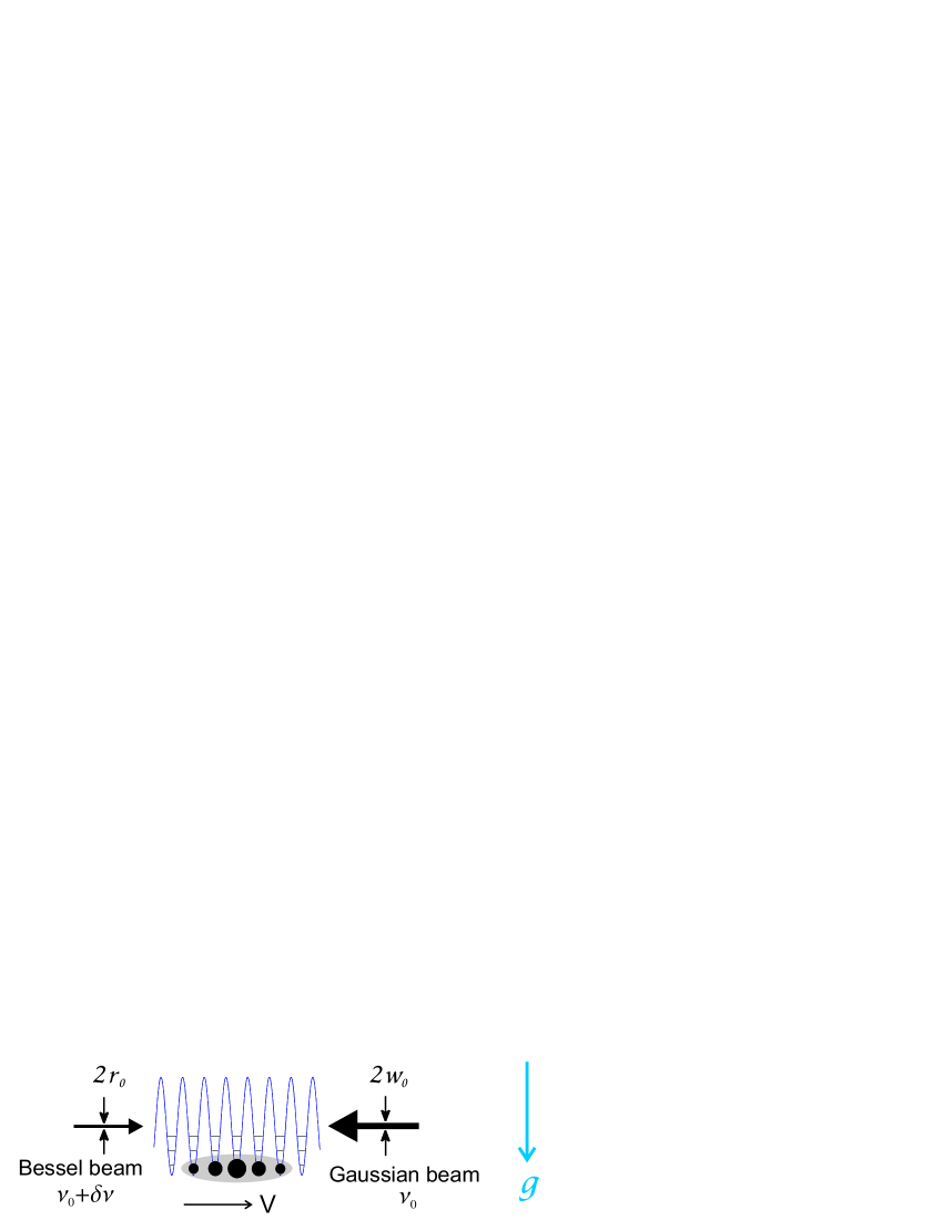
Figure 1: Scheme for atom transport. Two counterpropagating laser beams form a standing wave dipole trap. A BEC is loaded adiabatically into the vibrational ground state of this 1D optical lattice. A relative frequency detuning $\Delta\nu$ between the two laser beams results in a lattice motion at a velocity $v=\Delta\nu\cdot\lambda/2$ which drags along the trapped atoms. We chose the counterpropagating laser beams to consist of a Gaussian beam with diameter 2$w_{0}$ and a Bessel beam with a central spot diameter of 2$r_{0}$. The (in principle) diffraction-free propagation of the Bessel beam leads to tight radial confinement of the atoms over long distances, which supports the atoms against gravity during horizontal transport.

2 Basic Principle of Transport

Horizontal transport of atoms over larger distances holds two challenges: how to move the atoms and how to support them against gravity. Our approach here is to use a special 1D optical lattice trap, which is formed by a Bessel laser beam and a counterpropagating Gaussian beam. The lattice part of the trap moves the atoms axially, whereas the Bessel beam leads to radial confinement holding the atoms against gravity.

In brief, lattice transport works like this. We first load the atoms into a 1D optical lattice, which in general is a standing wave interference pattern of two counter propagating laser beams far red-detuned from the atomic resonance line (see Figure 1). Afterwards the optical lattice is carefully moved, “dragging” along the atoms. Upon arrival at the destination, the atoms are released from the lattice.

The lattice motion is induced by dynamically changing the relative frequency detuning $\Delta\nu$ of the two laser beams, which corresponds to a lattice velocity

$$v=\frac{\lambda}{2}\Delta\nu,$$ (1)

where $\lambda$ is the laser wavelength of the lattice.

In comparison to the classical notion of simply “dragging” along the atoms in the lattice, atom transport is more subtle on the quantum level. Here only momenta in multiples of two photon recoil momenta, $2\hbar k=4\pi\hbar/\lambda$ can be transferred to the atoms. This quantized momentum transfer can be understood in several ways, e.g. based on stimulated Raman transitions or based on the concept of Bloch-like oscillations in lattice potentials. For a more thorough discussion in this context the reader is referred to [14].

In order to prevent the atoms from falling in the gravitational field, the lattice has to act as an optical dipole trap in the radial direction. It turns out that for radial trapping, optical lattices formed by Bessel beams have a clear advantage over Gaussian beam lattices. To make this point clear, we now show, that a standard optical lattice based on Gaussian beams is not well suited for long distance transports on the order of 50 cm. During transport we require the maximum radial confining force $F_{\textrm{\scriptsize max}}$ to be larger than gravity $mg$, where $m$ is the atomic mass and $g\approx$ 9.81 m/s² is the acceleration due to gravity. For a Gaussian beam this is

$$F_{\textmd{\scriptsize max}}=\frac{3}{4\pi^{3}\sqrt{\textrm{e}}}\,\frac{\lambda^{3}}{c}\,\frac{\Gamma}{\Delta}\,\frac{P_{0}}{w(z)^{3}}>mg$$ (2)

where $\Gamma$ is the natural linewidth of the relevant atomic transition, $\Delta$ the detuning from this transition, $w(z)$ the beam radius and $P_{0}$ the total power of the beam. The strong dependence on the beam radius $w(z)$ suggests, that $w(z)=w_{0}\sqrt{1+(z/z_{\textrm{\scriptsize R}})^{2}}$ should not vary too much over the transport distance. If we thus require the Rayleigh range $z_{\textrm{\scriptsize R}}=\pi w_{0}^{2}/\lambda$ to equal the distance of 25 cm, the waist has to be $w_{0}\approx$ 260$\,\mu$m. For a lattice beam wavelength of e.g. $\lambda=830\,$nm, the detuning from the D-lines of ⁸⁷Rb is $\Delta\approx 2\pi\times 130\,$THz. To hold the atoms against gravity for all $z$, where $|z|<z_{\textrm{\scriptsize R}}$, a total laser power of $P_{0}\approx$ 10 W is needed, which is difficult to produce. In addition the spontaneous photon scattering rate

$$\Gamma_{scatt}=\frac{3}{8\pi^{3}\hbar}\,\frac{\lambda^{3}}{c}\,\left(\frac{\Gamma}{\Delta}\right)^{2}\,\frac{P_{0}}{w(z)^{2}}\\$$ (3)

would reach values on the order of $\Gamma_{\textrm{\scriptsize scatt}}=$ 2 s^-1. For typical transport times of 200 ms this means substantial heating and atomic losses.

A better choice for transport are zero order Bessel beams (Figure 2). They exhibit an intensity pattern which consists of an inner intensity spot surrounded by concentric rings and which does not change during propagation. In our experiments we have formed a standing light wave by interfering a Bessel beam with a counter-propagating Gaussian beam, giving rise to an optical lattice which is radially modulated according to the Bessel beam . Atoms loaded into the tightly confined inner spot of the Bessel beam can be held against gravity for moderate light intensities, which minimizes the spontaneous photon scattering rate. In comparison to the transport with a Gaussian beam, the scattering rate in a Bessel beam transport can be kept as low as 0.05 s^-1 by using the beam parameters of our experiment.

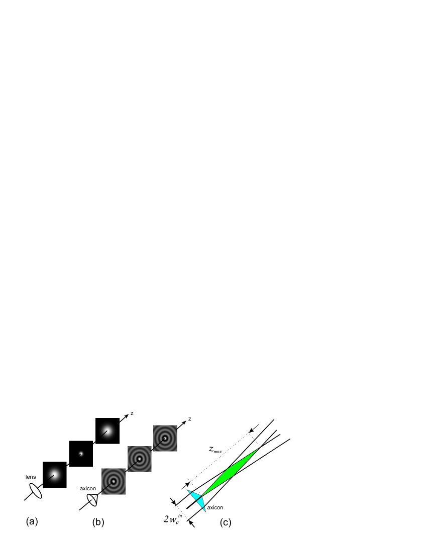
Figure 2: Gaussian and Bessel beams. (a) The radial intensity distribution of a Gaussian beam changes as it propagates. The smaller the waist $w_{0}$ of the beam, the higher its divergence (for a given wavelength). (b) Bessel beam: The radial distribution and in particular the radius of the central spot $r_{0}$ do not change with $z$ (see equation (8)). (c) Within a certain axial range $z_{max}$ a Bessel-like beam can be produced by illuminating an axicon lens with a collimated laser beam.

3 Bessel beams

Bessel beams are a solution of the Helmholtz equation and were first discussed and experimentally investigated about two decades ago [15, 16].

In cylindrical coordinates the electric field distribution of a Bessel beam of order $l$ is given by

$$E(r,\varphi,z) = E_{0}\ \ e^{i\beta z}\ e^{il\varphi}\ J_{l}(\alpha r)\ ,$$ (4)

where $J_{l}(\alpha r)$ is the Bessel function of the first kind with integer order $l$. The beam is characterized by the parameters $\alpha$ and $\beta$. In the following, we restrict the discussion to order $l=0$ which we have used in the experiment. By taking the absolute square of this expression one gets the intensity distribution given by

$$I(r,z)=I_{0}\;J_{0}^{2}(\alpha r),$$ (5)

where $\alpha$ determines the radius $r_{0}$ of the central spot via the first zero crossing of $J_{0}(\alpha r)$

$$r_{0}\approx{4.81\over 2\alpha}.$$ (6)

As pointed out before, $r_{0}$ and $I_{0}$ do not change with the axial position $z$. Because of this axial independence the Bessel beams are said to be “diffraction-free”.

Bessel-like beams were realized experimentally for the first time by illuminating a circular slit [16]. Since this method is very inefficient, two other ways are common nowadays. To generate Bessel beams of arbitrary order holographic elements, such as phase-gratings, are used [17]. In our setup we use a zero order Bessel beam, which can be produced efficiently by simply illuminating an axicon (conical lens) with a collimated laser beam [18]. How this comes about, can be understood by looking at the Fourier transform of the Bessel field

$$\widetilde{E}(k_{\bot},\varphi_{k},k_{z}) = \int d^{3}r~{}E(r,\varphi,z)e^{-ik_{\bot}r\cos(\varphi-\varphi_{k})}e^{-ik_{z}z}$$ (7)

$$\propto e^{il\varphi_{k}}~{}\delta(k_{z}-\beta)~{}\delta(k_{\bot}-\alpha).$$

Thus a Bessel beam is a superposition of plane waves with $(k_{\bot},k_{z})=(\alpha,\beta)$. The $\mathbf{k}$ - vectors of the plane waves all have the same magnitude $|\mathbf{k}|$ = $k$ = $2\pi/\lambda$ = $\sqrt{\alpha^{2}+\beta^{2}}$ and they are forming a cone with radius $k_{\bot}$ and height $k_{z}$. Using an axicon with apex angle $\delta$ and index of refraction $n$, $\alpha$ and $\beta$ are given by

$$\alpha=\frac{\pi(n-1)}{2\lambda\tan\delta/2}$$ (8)

and

$$\beta=\sqrt{k^{2}-\alpha^{2}}.$$ (9)

These experimentally produced Bessel beams are not ideal in the sense that their range $z_{\textrm{\scriptsize max}}=kw_{0}^{\textrm{\scriptsize in}}/\alpha$ is limited by the finite size (waist $w_{0}^{\textrm{\scriptsize in}}$) of the beam impinging on the axicon lens (see Figure 2(c)). Also, the intensity of the Bessel beams might not be independent of the axial coordinate $z$, as it is also determined by the radial intensity distribution of the impinging beam (e.g. see Figure 4(b)).

4 Experimental setup

We work with a ⁸⁷Rb-BEC in the internal state $|F=1,~{}m_{F}=-1\rangle$, initially held in a Ioffe-type magnetic trap with trap frequencies of $2\pi\,\nu_{x,y,z}$ = $2\pi\,$(7 Hz, 19 Hz, 20 Hz) [19, 20]. From the magnetic trap the condensate is adiabatically loaded in about 100 ms into the inner core of the 1D optical lattice formed by a Bessel beam of central spot radius $r_{0}=$ 36$\,\mu$m and a counter-propagating Gaussian beam with a waist of $w_{0}=$ 85$\,\mu$m. About 70 lattice sites are occupied with atoms in the vibrational ground state. The lattice periodicity is 415 nm, corresponding to the laser wavelength of 830 nm. For our geometry (see below) the total power needed for the Bessel beam to support the atoms against gravity is typically 200 mW, since only a few percent ($\approx$ 10 mW) of the total power are stored in the central spot. For the Gaussian beam a power of roughly 20 mW is chosen, leading to an optical trapping potential at the center ($r=0$) of $U(z)=-U_{0}+U_{\textrm{\scriptsize latt}}\sin^{2}(kz)$, where the lattice depth (effective axial trap depth) is $U_{\textrm{\scriptsize latt}}\approx$ 10$\,E_{\textrm{\scriptsize r}}$ and the total trap depth $U_{0}\approx$ 11$\,E_{\textrm{\scriptsize r}}$. Here $E_{\textrm{\scriptsize r}}=(\hbar k)^{2}/(2m)$ is the recoil energy.

The corresponding trap frequencies are $\nu_{\bot}=4.81\sqrt{U_{0}/(8mr_{0}^{2})}/(2\pi)$ = 97 Hz in the radial direction and $\nu_{z}=k\sqrt{2U_{\textrm{\scriptsize latt}}/m}/(2\pi)$ = 21 kHz in the axial direction. In order to better analyze the transport properties, we mostly perform round trips, where the atoms are first moved to a distance $D$ and then back to their initial spot, which lies in the field of vision of our CCD camera. Once back, the atoms are adiabatically reloaded into the Ioffe-type magnetic trap. To obtain the resulting atomic momentum distribution a standard absorption imaging picture is taken after sudden release from the magnetic trap and typically 12 ms of time-of-flight.

The lattice beams for the optical lattice are derived from a Ti:Sapphire-laser operating at 830 nm. The light is split into two beams, each of which is controlled in amplitude, phase and frequency with an acousto-optical modulator (AOM). For both AOMs the radio-frequency (RF) driver consists of a home-built 300 MHz programmable frequency generator, which gives us full control over amplitude, frequency and phase of the radio-wave at any instant of time. The frequency generator is based on an AD9854 digital synthesizer chip from Analog Devices and a 8-bit micro-controller ATmega162 from Atmel, on which the desired frequency ramps are stored and from which they are sent to the AD9854 upon request. After passing the AOMs, the two laser beams are mode-cleaned in single-mode fibers and converted into collimated Gaussian beams. One of the Gaussian beams passes the axicon lens (apex angle = 178^∘, radius = 25.4 mm, Del Mar Photonics) with a waist of $w_{0}^{\textrm{\scriptsize in}}=2\,$mm, producing the Bessel beam. From there the beam propagates towards the condensate, which -before transport- is located 5 cm away.

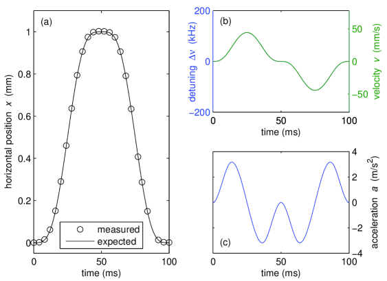
Figure 3: (a) Position, (b) velocity and (c) acceleration of the atomic cloud as a function of time for a typical transport sequence, here a round-trip over a short distance of 1mm. Piecewise defined cubic polynomials are used for the acceleration ramp (see appendix for an analytical expression). By integrating over time, velocity and position are obtained. The frequency detuning $\Delta\nu$, which is used to program the RF synthesizers, corresponds directly to the velocity $v$ via equation (1). The position ramp is compared with in-situ measurements of the cloud’s position (circles).

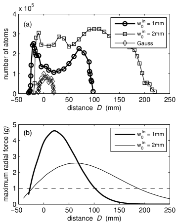
Figure 4: Long distance transports. (a) Shown is the number of remaining atoms after a round-trip transport (see Figure 3) over various one-way distances $D$. The first two data sets are obtained with two different Bessel beams which are created by illuminating an axicon with a Gaussian beam with a waist $w_{0}^{in}$ = 1 mm and 2 mm, respectively. The transport time $T$ was kept constant at $T=$130 ms and $T=$280 ms, respectively. The third data set (diamonds) corresponds to a transport in a Gaussian beam lattice (see text). The calculated maximum radial trapping force of the two Bessel beam lattice traps is shown in (b) in units of $mg$, where $g\approx$ 9.81 m/s² denotes the gravitational acceleration. The variation of the trapping force with distance is an imperfection of the Bessel beam and reflects its creation from a Gaussian beam. When the maximum radial force drops below 1$\,g$, gravity pulls the atoms out of the trap, as can be clearly seen in (a).

5 Transport of ultracold atoms

Figure 3 shows results of a first experiment, where we have transported atoms over short distances of up to 1 mm (round trip), so that they never leave the field of view of the camera. The atoms move perpendicularly to the direction of observation. In-situ images of the atomic cloud in the optical lattice are taken at various times during transport and the center of mass position of the cloud is determined. As is clear from Figure 3(a) we find very good agreement between the expected and the measured position of the atoms. In Figure 3(b) and 3(c), calculations are shown for the corresponding velocity $v(t)$ and acceleration $a(t)$ of the optical lattice, respectively. As discussed before (see equation (1)), the velocity $v$ of the lattice translates directly into a relative detuning $\Delta\nu$ of the laser beam, which we control via the AOMs. In order to suppress unwanted heating and losses of atoms during transport, we have chosen very smooth frequency ramps $\Delta\nu(t)$ such that the acceleration is described by a cubic spline interpolation curve which is continuously differentiable (details are given in the appendix). In this way also the derivative of the acceleration (commonly called the jerk) is kept small.

In the next set of experiments we have extended the atomic transport to more macroscopic distances of up to 20 cm (40 cm round trip), where we moved the atoms basically from one end of the vacuum chamber to the other and back. However, the transport distance was always limited by the finite range $z_{\textrm{\scriptsize max}}$ of the Bessel beam (see Figure 2(c) and Figure 4). As shown in Figure 4, the total number of atoms abruptly decreases at the axial position, where the maximum radial force drops below gravity. It is also clear from the figure, how the range of the Bessel beam is increased by enlarging the waist $w_{0}^{\textrm{\scriptsize in}}$ of the incoming Gaussian beam. Of course, for a given total laser power, the maximum radial force decreases as the Bessel beam diameter is increased. For the transport distances of 12 cm and 20 cm the total power in the Bessel beam was approximately 400 mW. For comparison, we have also transported atoms with a lattice formed by two counter-propagating Gaussian beams (see Fig. 4 (a)). For this transport both laser beams have a Rayleigh range of $z_{R}\approx 2\,$cm corresponding to a waist of 70 $\mu$m. The laser power of the two beams was $\approx 130\,$mW and $\approx 35\,$mW, respectively. We observe a sudden drop in atom number when the transport distance exceeds the Rayleigh range. Using the scaling law given in equation (2) it should be clear that transports of atoms over tens of cm with a Gaussian lattice is hard to achieve.

Interestingly, the curve corresponding to the Bessel beam with waist $w_{0}^{\textrm{\scriptsize in}}$ = 1 mm in Figure 4(a) exhibits a pronounced minimum in the number of remaining atoms at a distance of about 3 cm. The position of this minimum coincides with the position, where the lattice depth has a maximum (see Figure 4(b)). This clearly indicates, that high light intensities adversely affect atom lifetimes in the lattice. Although we have not studied in detail the origin of the atomic losses in this work, they should partially originate from spontaneous photon scattering and 3-body recombination. In the deep lattice here (60$\,E_{\textrm{\scriptsize r}}$) the calculated photon scattering rate is $\Gamma_{\textrm{\scriptsize scatt}}=$ 0.4 s^-1. The tight lattice confinement leads to a high calculated atomic density of $n_{0}\approx 2\ 10^{14}$ cm^-3. Adopting $L=5.8\times 10^{-30}$cm⁶/s as rate coefficient for the three body recombination [21], we expect a corresponding loss rate $Ln_{0}^{2}=$0.3 s^-1.

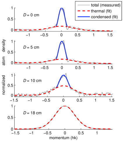
Figure 5: Transporting BEC. Shown are the momentum distributions (thin black lines) of the atoms after a return-trip transport over various one-way distances $D$. A bimodal distribution (a blue parabolic distribution for the condensed fraction and a red Gaussian distribution for the thermal fraction) is fit to the data. For $D$ below 10cm a significant fraction of the atomic cloud is still condensed. For $D=$18 cm ($\approx$ the limit in our experiments) only a thermal cloud remains, however, with a temperature below the recoil limit (T $<$ 0.2$\,E_{r}/k_{B}$ $\approx$ 30 nK).

Figure 6: Critical acceleration in lattice. (a) For several round-trip transports with varying maximum acceleration $a$ and lattice depth (see legend), the number of remaining atoms after transport is shown. As the maximum acceleration exceeds a critical value, the number of atoms starts to drop significantly. We define a critical acceleration as the maximum acceleration for transports in which 50$\%$ of the atoms still reach their final destination. This critical acceleration is shown as a function of the lattice depth in (b). The experimentally determined values are compared with the limit expected from classical considerations: $a_{crit}=U_{\textrm{\scriptsize latt}}k/m$.

In Figure 5 we have studied the transport of a BEC, which is especially sensitive to heating and instabilities. It is important to determine, whether the atoms are still Bose-condensed after the transport and what their temperature is afterwards. Figure 5 shows momentum-distributions for various transport distances $D$, which were obtained after adiabatically reloading the atoms into the magnetic trap by ramping down the lattice and subsequent time-of-flight measurements.

Before discussing these results, we point out that loading the BEC adiabatically into the stationary optical lattice is already critical. We observe a strong dependence of the condensate fraction on the lattice depth. For too low lattice depths most atoms fall out of the lattice trap due to the gravitational field. For too high lattice depths all atoms are trapped but the condensate fraction is very small. One explanation for this is that high lattice depths lead to the regime of 2D pancake shaped condensates where tunnelling between adjacent lattice sites is suppressed. Relative dephasing of the pancake shaped condensates will then reduce the condensate fraction after release from the lattice. We obtain the best loading results for a 11$\,E_{r}$ deep trap, where we lose about 65$\%$ of the atoms, but maximize the condensate fraction. Because high lattice intensities are detrimental for the BEC, we readjust the power of the lattice during transport, such that the intensity is kept constant over the transport range. The adjustments are based on the calculated axial intensity distribution of the Bessel beam. In this way we reach transport distances for BEC of 10 cm. We believe, that more sophisticated fine tuning of the power adjustments should increase the transport length considerably. After transport distances of $D$ = 18 cm (36 cm round trip) the atomic cloud is thermal. Its momentum spread, however, is merely 0.3$\,\hbar k$, which corresponds to a temperature of 30 nK. Additionally, we want to point out, that the loss of atoms due to the transport is negligible ($<$10$\%$) compared to the loss through loading and simply holding in such a low lattice potential ($\approx 65\%$).

An outstanding feature of the lattice transport scheme is the precise positioning of the atomic cloud. Aside from uncontrolled phase shifts due to residual mechanical noise, such as vibrating optical components, we have perfect control over the relative phase of the lattice lasers with our RF / AOM setup. This would in principle result in an arbitrary accuracy in positioning the optical lattice. We have experimentally investigated the positioning capabilities in our setup. For this we measured in many runs the position of the atomic cloud in the lattice after it had undergone a return trip with a transport distance of $D=$ 10 cm. The position jitter, i.e. the standard deviation from the mean position, was slightly below 1$\,\mu$m. For comparison, we obtain very similar values for the position jitter when investigating BECs in the lattice before transport. Hence the position jitter introduced through the transport scheme is negligible.

Another important property of the lattice transport scheme is its high speed. For example, for a transport over 20 cm (40 cm round trip) with negligible loss, a total transport time of 200 ms turns out to be sufficient. This is more than an order of magnitude faster than in the MIT experiment [4], where an optical tweezer was mechanically relocated. The reason for this speed up as compared to the optical tweezer is mainly the much higher axial trapping frequency of the lattice and the non-mechanical setup.

In order to determine experimentally the lower limit of transportation time we have investigated round-trip transports ($D=$ 5 mm), where we have varied the maximum acceleration and the lattice depth (Figure 6(a)). The number of atoms, which still remain in the lattice after transport, is measured. As soon as the maximum acceleration exceeds a critical value, the number of atoms starts to drop. For a given lattice depth, we define a critical acceleration $a_{crit}$ as the maximum acceleration of the particular transport where 50$\%$ of the atoms still reach their final destination. Figure 6(b) shows the critical acceleration $a_{\textrm{\scriptsize crit}}$ as a function of lattice depth. The upper bound on acceleration observed here can be understood from classical considerations. In our lattice the maximum confining force along the axial direction is given by $U_{latt}k$, where $k$ is the wave vector of the light field. Thus in order to keep an atom bound to the lattice, we require the acceleration $a$ to be small enough such that

$$ma<U_{\textrm{\scriptsize latt}}k.$$ (10)

Our data in Figure 6 are in good agreement with this limit .

There is in principle also a lower bound on the acceleration, which is due to instabilities exhibited by BECs with repulsive interactions loaded into periodic potentials [23, 24, 25, 26]. Due to the fact that these instabilities mainly occur at the edge of the Brillouin zones, the time spent in this critical momentum range should be kept small. For our lattice parameters nearly half of the Brillouin zone is an unstable region, where the lifetime of the BEC is only on the order of 10 ms [25]. Thus we tend to sweep through the Brillouin zone in much less than $\Delta t=$ 20 ms, which corresponds to an acceleration of $a=\dot{v}\,\gg\,2v_{r}/\Delta t\simeq$ 0.6 m/s². In this way BECs may be transported without introducing too much heating through these instabilities.

In contrast to acceleration, the transport velocity in our experiment is only technically limited due to the finite AOM bandwidth. As discussed before, the lattice is set in motion by introducing a detuning between the two beams via AOMs (equation (1)). For detunings exceeding the bandwidth of the AOM, the diffraction efficiency of the modulator starts to drop significantly. Consequently the lattice confinement vanishes, and the atoms are lost. In our setup we can conveniently reach velocities of up to $v=6\,$m/s $\approx$ 1100$\,v_{r}$, corresponding to a typical AOM bandwidth of 15 MHz. This upper bound actually limits the transport time for long distance transports ($D$ $>$ 5 cm).

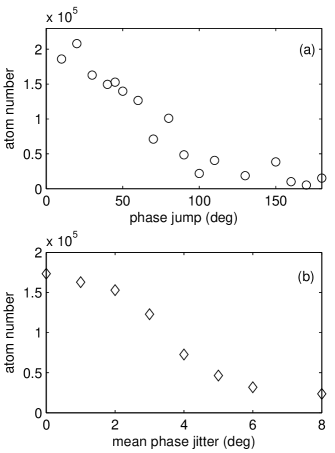
Figure 7: Stability requirements for transport. Sudden phase jumps are introduced in the relative phase of the two counterpropagating lattice laser beams. The corresponding abrupt displacements of the optical lattice lead to heating and loss of the atoms. We measure the number of atoms which remain in the lattice after transport. (a) Data obtained after a single relative phase jump of variable magnitude. (b) A phase jitter (200 positive Poissonian-distributed phase jumps with a variable mean value) is introduced during transport. Mean values on the order of a few degrees already lead to a severe loss of atoms.

Finally we have investigated the importance of phase stability of the optical lattice for the transport (see Figure 7). For this we purposely introduced sudden phase jumps during transport to one of the lattice beams. The timescale for the phase jumps, as given by AOM response time of about 100 ns, was much smaller than the inverse trapping frequencies. The phase jumps lead to abrupt displacements of the optical lattice, causing heating and loss of atoms. In Figure 7(a) the atomic losses due to a single phase jump during transport are shown. Phase jumps of 60^∘ typically induce a 50 % loss of atoms. For continuous phase jitter (see Figure 7(b)) the sensitivity is much larger.

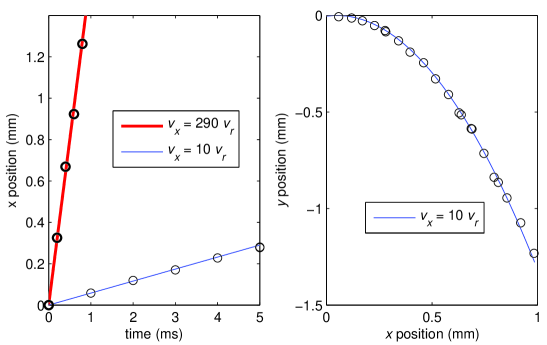
Figure 8: Atom catapult. After acceleration in $x$-direction and subsequent release from the lattice, the position of the atomic cloud is tracked as it flies ballistically through the field of view of the CCD camera. Shown are two data sets where atoms were accelerated to velocities of either $v_{\textrm{\scriptsize x}}$ = 10$\,v_{\textrm{\scriptsize r}}$ or $v_{\textrm{\scriptsize x}}$ = 290$\,v_{\textrm{\scriptsize r}}$. (a) The horizontal position $x$ as a function of time. (b) For the slower cloud ($v_{\textrm{\scriptsize x}}$ = 10$\,v_{\textrm{\scriptsize r}}$) a parabolic trajectory $y=-g/2\cdot(x/v_{\textrm{\scriptsize x}})^{2}$ is observed as it falls under the influence of gravity.

6 Atom catapult

In addition to transport of ultracold atoms, acceleration of atoms to precisely defined velocities is another interesting application of the moving optical lattice. For instance, it could be used to study collisions of BECs with a very high but well defined relative velocity, similar to the experiments described in [27, 28]. As already shown above, we have precise control to impart a well defined number of up to 1100 photon recoils to the atoms. This corresponds to a large kinetic energy of $k_{B}\,\times\,$200 mK. At the same time the momentum spread of the atoms is about 1/3 of a recoil (see Figure 5). To illustrate this, we have performed two sets of experiments, where we accelerate a cloud of atoms to velocities $v=10\,v_{r}$ and $v=290\,v_{r}\approx$ 1.6 m/s. After adiabatic release from the lattice, we track their position in free flight (see Figure 8). Initially the atomic cloud is placed about 8 cm away from the position of the magnetic trap. It is then accelerated back towards its original location. Before the atoms pass the camera’s field of vision, the lattice beams are turned off within about 5 ms, to allow a ballistic flight of the cloud. Using absorption imaging the position of the atomic cloud as a function of time is determined. The slope of the straight lines in Figure 8(a) corresponds nicely to the expected velocity. However, due to a time jitter problem, individual measurements are somewhat less precise than one would expect. For $v=10$ $v_{r}$, Figure 8(b) shows the trajectory of the ballistic free fall of the atoms in gravity.

7 Conclusion

In conclusion, we have realized a long distance optical transport for ultracold atoms, using a moveable standing wave dipole trap. With the help of a diffraction-free Bessel beam, macroscopic distances are covered for both BEC and ultracold thermal clouds. The lattice transport features a fairly simple setup, as well as a fast transport speed and high positional accuracy. Limitations are mainly technical and leave large room for improvement. In addition to transport, the lattice can also be used as an accelerator to impart a large but well defined number of photon recoils to the atoms.

8 Acknowledgements

We want to thank U. Schwarz for helpful information on the generation of Bessel beams and for lending us phase-gratings for testing purposes. Furthermore we thank R. Grimm for discussions and support. This work was supported by the Austrian Science fund (FWF) within SFB 15 (project part 17) and the Tiroler Zukunftsstiftung.

Appendix: Transport Ramp

We give here the analytic expression for the lattice acceleration $a(t)$ as a function of time $t$ which was implemented in our experiments (see for example Figure 3). $a(t)$ is a smooth piecewise defined cubic polynomial,

$$\!\!\!\!\!\!\!\!\!\!\!\!\!\!\!\!\!\!\!\!\!\!\!\!\!\!\!a(t)=\left\{\begin{array}[]{r @{\quad{\mbox{for}}\quad} l}\frac{D}{T^{2}}\;(-\frac{7040}{9}(\frac{t}{T})^{3}+320(\frac{t}{T})^{2})&0<t\leq T/4\\ \frac{D}{T^{2}}\;(\frac{3200}{9}(\frac{t}{T})^{3}-\frac{1600}{3}(\frac{t}{T})^{2}+\frac{640}{3}\frac{t}{T}-\frac{160}{9})&T/4<t\leq 3T/4\\ \frac{D}{T^{2}}\;(-\frac{7040}{9}(\frac{t}{T})^{3}+\frac{6080}{3}(\frac{t}{T})^{2}-\frac{5120}{3}\frac{t}{T}+\frac{4160}{9})&3T/4<t\leq T\\ \end{array}\right.$$

Here, $D$ is the distance over which the lattice is moved and $T$ is the duration of the transport. From $a(t)$ both the velocity $v(t)$ and the location $x(t)$ may be derived via integration over time. Our choice for the acceleration $a(t)$ features a very smooth transport. The acceleration $a(t)$ and its derivative $\dot{a}(t)$ are zero at the beginning ($t=0$) and at the end ($t=T$) of the transport. At $t=T/4$ and $t=3T/4$ the absolute value of the acceleration reaches a maximum.

References

References

- [1] Folman R, Krüger P, Schmiedmayer J, Denschlag J and Henkel C 2002 Adv. At. Mol. Opt. Phys. 48, 263-352
- [2] Greiner M, Bloch I, Hänsch T W and Esslinger T 2001 Phys. Rev. A 63 031401
- [3] Lewandowski H J, Harber D M, Whitaker D L and Cornell E A 2002 Phys. Rev. Lett. 88 070403
- [4] Gustavson T L, Chikkatur A P, Leanhardt A E, Görlitz A, Gupta S, Pritchard D E and Ketterle W 2002 Phys. Rev. Lett. 88, 020401
- [5] Kasevich M and Chu S 1991 Phys. Rev. Lett. 67 000181
- [6] Berg-Sørensen K and Mølmer K 1998 Phys. Rev. A 58 1480
- [7] Pötting S, Cramer M, Schwalb C H, Pu H and Meystre P 2001 Phys. Rev. A 64 023604
- [8] Dahan M B, Peik E, Reichel J, Castin Y and Salomon C 1996 Phys. Rev. Lett. 76 4508-4511
- [9] Morsch O, Müller J H, Cristiani M, Ciampini D and Arimondo E 2001 Phys. Rev. Lett. 87 140402
- [10] Morsch O, Oberthaler M 2006 Phys. Mod. Phys. 78 179-215
- [11] Kuhr S, Alt W, Schrader D, Müller M, Gomer V and Meschede D 2001 Science 293 278
- [12] Mandel O, Greiner M, Widera A, Rom T, Hänsch T W and Bloch I 2003 Phys. Rev. Lett. 91 010407
- [13] Cizmar T, Garces-Chavez V, Dholakia K and Zemanek P 2005 Appl. Phys. Lett. 86 174101
- [14] Hecker Denschlag J, Simsarian J E, Häffner H, McKenzie C, Browaeys A, Cho D, Helmerson K, Rolston S L and Phillips W D 2002 J. Phys. B 35 3095-3110
- [15] Durnin J 1987 J. Opt. Soc. Am. B 4 651-654
- [16] Durnin J, Miceli J J and Eberly J H 1987 Phys. Rev. Lett. 58 1499-1501
- [17] Niggl L, Lanzl T and Maier M 1997 J. Opt. Soc. Am. A 14 27-33
- [18] Niggl L 1999 PhD thesis Logos Berlin ISBN 3-89722-319-8
- [19] Thalhammer G, Winkler K, Lang F, Schmid S, Grimm R and Hecker Denschlag J 2006 Phys. Rev. Lett 96 050402
- [20] Thalhammer G, Theis M, Winkler K, Grimm R and Hecker Denschlag J 2005 Phys. Rev. A 71 033403
- [21] Söding J, Guéry-Odelin D, Desbiolles P, Chevy F, Inamori H and Dalibard J 1999 Appl. Phys. B 69 257-261
- [22] Peik E, Dahan M B, Bouchoule I, Castin Y and Salomon C 1997 Phys. Rev. A 55 4
- [23] Choi D I and Niu Q 1999 Phys. Rev. Lett. 82 2022
- [24] Wu B and Niu Q 2003 New J. Phys. 5 104.1-104.24
- [25] Fallani L, De Sarlo L, Lye J E, Modugno M, Saers R, Fort C and Inguscio M 2004 Phys. Rev. Lett. 93 140406
- [26] Cristiani M, Morsch O, Malossi N, Jona-Lasinio M, Anderlini M, Courtade E and Arimondo E 2004 Opt. Express 12 4
- [27] Thomas N R, Kjaergaard N, Julienne P S and Wilson A C 2004 Phys. Rev. Lett. 93 173201
- [28] Buggle C, L onard J, Klitzing W von and Walraven J T M 2004 Phys. Rev. Lett. 93 173202