Electric Dipole Induced Spin Resonance in Disordered Semiconductors

Abstract

One of the hallmarks of spintronics is the control of magnetic moments by electric fields enabled by strong spin-orbit interaction (SOI) in semiconductors. A powerful way of manipulating spins in such structures is electric dipole induced spin resonance (EDSR), where the radio-frequency fields driving the spins are electric, and not magnetic like in standard paramagnetic resonance. Here, we present a theoretical study of EDSR for a two-dimensional electron gas in the presence of disorder where random impurities not only determine the electric resistance but also the spin dynamics via SOI. Considering a specific geometry with the electric and magnetic fields parallel and in-plane, we show that the magnetization develops an out-of-plane component at resonance which survives the presence of disorder. We also discuss the spin Hall current generated by EDSR. These results are derived in a diagrammatic approach with the dominant effects coming from the spin vertex correction, and the optimal parameter regime for observation is identified.

The field of spintronicsAwschalom et al. (2002); Zutic et al. (2004) focuses on the interplay between spin and charge degrees of freedom of the electron. The relativistic effects responsible for the coupling between spin and orbital motion can be strongly enhanced in solids due to band structure effects, with III-V semiconductors showing a particularly strong spin-orbit interaction (SOI) resulting in zero-field spin splittings. For instance, bulk inversion asymmetry gives rise to Dresselhaus SOIDresselhaus (1955), while structural inversion asymmetry occurring in heterostructures gives rise to Rashba SOIRashba (1960). The strength of such SOIs can be varied over a wide range which offers the advantage to control magnetic moments with electric fields. A well-known and particularly powerful way of manipulating spins in such structures is electric dipole induced spin resonance (EDSR)Bell (1962); Melnikov and Rashba (1972); Dobrowolska et al. (1984); Merkt et al. (1986); Kato et al. (2004a); Rashba and Efros (2003a); Schulte et al. (2005), where the radio frequency (rf) fields coherently driving the spins are electric, and not magnetic like in standard paramagnetic resonanceEdelstein (1993); Erlingsson et al. (2005). The advent of materials with tailored SOIAwschalom et al. (2002) has sparked intense interest in a variety of spin orbit effects and its applications such as spin currentsD’yakonov and Perel (1971); Murakami et al. (2004); Sinova et al. (2004); Kato et al. (2004b); Sih et al. (2005), gate-controlled SOI effectsSalis et al. (2001); Miller et al. (2003); Rashba and Efros (2003b); Kato et al. (2003), spin relaxation in quantum dotsElzerman et al. (2004); Kroutvar et al. (2004); Golovach et al. (2004), zitterbewegungSchliemann et al. (2005), spin-based quantum information processingAwschalom et al. (2002); Loss and DiVincenzo (1998), and, in particular, EDSRKato et al. (2004a); Schulte et al. (2005); Rashba and Efros (2003a), which is the focus of this work.

Experimental indication for EDSR was recently reported for semiconductor epilayers using an in-plane electric rf fieldKato et al. (2004a) (with the magnetic field applied out of plane). In this geometry, spin coupling to the electric field is much stronger than when the electric field is applied along the growth directionRashba and Efros (2003a). Further, a recent experiment in two-dimensional systems with cavities showed clearer signals for the configuration with electric and magnetic fields perpendicular to each other, while in the parallel one the observed resonance feature presented puzzlesSchulte et al. (2005).

Systems of particular importance are heterostructures forming a two-dimensional electron gas (2DEG), such as GaAs semiconductors. Here, the Rashba SOI is linear in momentum and provides an effective internal magnetic field about which the spin precesses. Realistic 2DEGs, moreover, contain disorder leading to momentum scattering which is responsible not only for the finite electric resistance but also for spin relaxation due to randomization of the internal fieldD’yakonov and Perel (1972); Dyakonov and Perel (1984). Unlike for the conventional paramagnetic settingEdelstein (1993) no microscopic study of EDSR in such systems is available, but would be highly desirable, also in view of the recent experimental activities. However, the interplay between SOI and disorder in orbital space can be quite subtle, as was fully appreciated only recently in a number of experimental and theoretical studies on spin currentsKato et al. (2004b); Sih et al. (2005); Inoue et al. (2004); Mishchenko et al. (2004); Dimitrova (2005); Chalaev and Loss (2005). There, it turned out that the intrinsic spin Hall effectSinova et al. (2004) in GaAs 2DEGs due to Rashba SOI does not survive the presence of disorder, which, technically speaking, results from an unusual cancellation of vertex correctionsInoue et al. (2004); Mishchenko et al. (2004); Dimitrova (2005); Chalaev and Loss (2005). Consequently, spin currents in these systems are dominated by other (extrinsic) effectsD’yakonov and Perel (1971); Sih et al. (2005); Engel et al. (2005). Similar concerns, for instance, apply to conclusions reached for EDSR in clean systemsRashba and Efros (2003a). Thus, the role of disorder needs to be examined carefully, and, in doing so, we show here that EDSR survives impurity scattering but acquires a line shape that is determined by disorder and SOI.

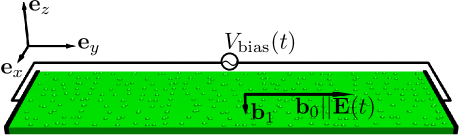
Figure 1: Setup for electric dipole induced spin resonance (EDSR). The disordered two-dimensional electron gas (2DEG) is placed in the xy-plane (green area). An a.c. bias $V_{\mathrm{bias}}(t)$ with frequency $\omega$ generates an electric a.c. field $\mathbf{E}(t)$ along ${\bf e}_{y}$ which is in-plane and parallel to the externally applied magnetic field $\mathbf{b}_{0}=g\mu_{B}\mathbf{B}_{0}/2$ (assumed to be static). As a consequence of the orbital motion of the electron induced by $\mathbf{E}(t)$, the Rashba spin orbit interaction generates an ’internal’ magnetic a.c. field $\mathbf{b}_{1}$ which is in-plane and perpendicular to the momentum of the electron and thus to $\mathbf{b}_{0}$ (ignoring disorder). This configuration of fields is now analogous to conventional paramagnetic resonance and allows manipulation of the electron spin.

We consider a geometry as shown in Fig. 1, where the electric rf field and the static external magnetic field are parallel and both in the plane of the 2DEG. At resonance, the spin polarization (magnetization) acquires a non-zero out-of-plane component. This we show first for a clean 2DEG by deriving an effective Bloch equation. Turning then to 2DEGs with disorder we treat the electric rf field in linear response and obtain for the magnetization a Lorentzian resonance whose width is given by a generalized D’yakonov-Perel spin relaxation rate. In addition, we find a shift of the resonance due to disorder and SOI which gives rise to an effective g-factor that depends on the magnetic field. Using a standard diagrammatic approach to treat SOI and disorder systematically, we find that it is the spin vertex correction (coming from disorder) that leads to the resonance, in stark contrast to zero frequency where the spin vertex vanishesEdelstein (1990). Assuming realistic system parameters we identify the most promising regime for the experimental observation of EDSR. Finally, we discuss the spin Hall current and show its relation to EDSR.

I The model

The 2DEG consists of non-interacting electrons of mass m and charge e which are subject to a random impurity potential $V$. In addition, we allow for a general SOI $\mathbf{\Omega}(\mathbf{p})\cdot\boldsymbol{\sigma}$ linear in momentum $\mathbf{p}$ and a static external magnetic field $\mathbf{B}_{0}$ applied in-plane, as well as a time-dependent electric field $\mathbf{E}(t)$ applied as a bias along $\mathbf{B}_{0}$, see Fig. 1. The Hamiltonian for this system reads

$$H=\frac{1}{2m}\left(\mathbf{p}-\frac{e}{c}\mathbf{A}\right)^{2}+\mathbf{\Omega}(\mathbf{p})\cdot\boldsymbol{\sigma}+(\mathbf{b}_{0}+\mathbf{b}_{1}(t))\cdot\boldsymbol{\sigma}+V,$$ (1)

where $\mathbf{b}_{1}(t)=-\frac{e}{c}\mathbf{\Omega}\left(\mathbf{A}(t)\right)$ is the rf part of the internal ’magnetic’ field induced by the electric field via SOI, and $\mathbf{A}(t)=-c\int^{t}dt^{\prime}\mathbf{E}(t^{\prime})$ is the associated vector potential, c being the speed of light. The Zeeman term contains $\boldsymbol{b}_{0}=g\mu_{B}\mathbf{B}_{0}/2$ and the Pauli matrices $\sigma^{i}$, $i=1,2,3$, while $\Omega(\mathbf{p})$ is the ’zero-field spin splitting’ due to the internal SOI field.

II Effective Bloch equation for the clean system

We show now that for the described setup the dynamics of the electron spin exhibits resonant behaviour (EDSR) generated by the electric rf field $\mathbf{E}(t)$. Starting with the simple case of no disorder ($V=0$), we derive a Bloch equation for the spin dynamics (for weak SOI), from which the EDSR property immediately follows. We begin by noting that the density matrix $\rho(t)$ is diagonal in momentum space, and its elements can be expanded in the spin basis as $\rho(\mathbf{p},t)=\sum_{\nu=0}^{3}s^{\nu}(\mathbf{p},t)\sigma^{\nu}$, where $\sigma^{0}=1$. The expectation value of the spin is then $\langle\sigma^{i}(t)\rangle=\int d^{2}p\;s^{i}(\mathbf{p},t)/(2\pi)^{2}\equiv S^{i}(t)$, where $\int s^{0}d^{2}p/(2\pi)^{2}=1$ due to normalization. [Henceforth, we refer to $S^{i}(t)$ as polarization, becoming the magnetization when multiplied with the Bohr magneton $\mu_{B}$.] In momentum space the symmetry is broken by the small SOI term such that the coefficients decompose into an isotropic and a small anisotropic part, $s^{i}(\mathbf{p},t)=\overline{s}^{i}(p,t)+\Delta s^{i}(\mathbf{p},t)$. Averaging the von Neumann equation for $\rho({\mathbf{p}},t)$ over directions of $\mathbf{p}$ we obtain

$$\dot{\bar{\mathbf{s}}}(p,t)=\frac{2}{\hbar}(\mathbf{b}_{0}+\mathbf{b}_{1}(t))\times\mathbf{\bar{s}}(p,t),$$ (2)

where we have dropped the angular average of $\mathbf{\Omega}(\mathbf{p})\times(\overline{\mathbf{s}}(p,t)+\Delta\mathbf{s}(\mathbf{p},t))$ since it is higher order in the SOI. Eq. (2) is now recognized as a Bloch equation describing spin resonance. Indeed, specializing henceforth to Rashba SOI $\Omega(\mathbf{p})=\alpha\mathbf{p}\times\mathbf{e}_{z}$, where $\mathbf{e}_{z}$ is a unit vector along the confinement axis, and taking $\mathbf{E}$ in the plane along $\mathbf{b}_{0}||\mathbf{e}_{y}$ results in the standard resonance setupCohen-Tannoudji et al. (1977) with an oscillating internal field $\mathbf{b}_{1}(t)\propto\mathbf{E}\times\mathbf{e}_{z}\perp\mathbf{B}_{0}$. Tuning $\mathbf{E}(t)$ to resonance, i.e. to frequency $\omega=\omega_{L}$, with $\omega_{L}=g\mu_{B}B_{0}$ being the Larmor frequency, the spin starts to precess around the x-axis (in the yz-plane) with a Rabi frequency $\omega_{R}=b_{1}/\hbar=eE_{0}\alpha/\hbar\omega_{L}$ given by the amplitude of the electric field $E_{0}$.

III Polarization of the Disordered 2DEG in Linear Response

Having established the existence of EDSR for the clean system we turn now to the realistic case of a disordered 2DEG. For this we assume a dilute random distribution of short-ranged scatterers with the disorder average $\overline{V(\mathbf{x})V(\mathbf{x}^{\prime})}=(m\tau)^{-1}\delta(\mathbf{x}-\mathbf{x}^{\prime})$ taken to be $\delta$-correlated and proportional to the mean free time $\tau$ between elastic scattering events. The interplay between SOI and disorder can then be characterized by the dimensionless parameter $x=2p_{F}\alpha\tau/\hbar$ measuring the precession angle around the internal field $2p_{F}\alpha/g\mu_{B}$ between scatterings.

For $A=0$ and $V=0$ the eigenenergies of H become $E_{s}(\mathbf{p})=p^{2}/2m+s\,b_{\mathrm{eff}}(\mathbf{p})$, with $s=\pm 1$ and the effective magnetic field $\mathbf{b}_{\mathrm{eff}}(\mathbf{p})=\alpha\mathbf{p}\times\mathbf{e}_{z}+\mathbf{b}_{0}$. In the corresponding retarded (advanced) Green functions

$$G^{R/A}(\mathbf{p},E)=\frac{1}{2}\sum_{s=\pm 1}\frac{1+s\frac{\mathbf{b}_{\mathrm{eff}}(\mathbf{p})}{b_{\mathrm{eff}}(\mathbf{p})}\cdot\boldsymbol{\sigma}}{E-E_{s}(\mathbf{p})\pm i/2\tau},$$ (3)

the disorder manifests itself as a finite self-energy term $i/2\tau$ generated by the disorder average. In the self-consistent Born approximation $\tau$ is independent of momentum due to the short range nature of $V$. We have also checked that a renormalization of the Zeeman splitting, i.e. matrix valued corrections, are of order $b_{0}/E_{F}$ and can be neglected as the Fermi energy $E_{F}$ is taken to be the largest energy scale. Thus, the averaged Green function is given by (3) with the standard isotropic and spin independent term $i/2\tau$Rammer (1998).

We turn now to the explicit calculation of the spin polarization (magnetization/$\mu_{B}$) $S^{i}(\omega)$ (per unit area) at frequency $\omega$, induced by the Fourier transform of the electric field $\mathbf{E}(\omega)$. Working in the linear response regime we start from the Kubo formula for $S^{i}(\omega)$ averaged over disorder and evaluate it using standard diagrammatic techniques. In Ref. Edelstein (1990) such a calculation was performed for the static ($\omega=0$) and zero field ($\mathbf{B}_{0}=0$) case, where, as a simplifying feature, the spin vertex correction turned out to vanish. For finite frequencies, however, this is no longer the case, and, as we shall sketch now, it is this vertex correction which leads to a finite out-of-plane polarization $S^{3}(\omega)$ at resonance $\omega=\omega_{L}$. To be specific, for $\hbar\omega\ll E_{F}$ the polarization becomes

$$S^{i}(\omega)=\frac{-eE_{j}(\omega)}{2\pi}\mathrm{Tr}\left\{G^{A}(q,E_{F})\;\Sigma^{i}(\omega)\>G^{R}(q,E_{F}+\omega)\;v_{j}\right\},$$ (4)

where summation over repeated indices is implied. Here, the velocity operator $v_{j}=(i/\hbar)[H,x_{j}]=p_{j}/m+\alpha(\mathbf{e}_{z}\times\boldsymbol{\sigma})_{j}$ contains the usual spin-dependent term, and $\mathrm{Tr}\rightarrow\int d^{2}q/(2\pi)^{2}\,\mathrm{tr}$ denotes momentum integration and tracing over spin states. In Eq.(4) we introduced the spin vertex correction $\Sigma(\omega)$ determined by the diagrammatic equation given in Fig. 2,

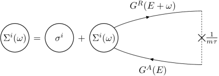
Figure 2: Diagrammatic equation for the spin vertex correction $\Sigma(\omega)$. Iterating the equation for $\Sigma^{i}(\omega)$ generates the ladder diagrams accounting for the dominant contribution of the impurity scattering (denoted by a cross) to the Kubo formula Eq. (4). The impurities causing momentum scattering of the electron are assumed to be short-ranged, isotropic, spin-independent, and randomly distributed in the 2DEG. Here, $\sigma^{i}$ denotes the Pauli matrix for the ith component of the electron spin, $G^{R/A}(E)$ is the retarded (advanced) Green function averaged over disorder (see Eq. 3), and $\tau$ is the mean-free-time between scattering events.

where the cross denotes the insertion of a factor $1/m\tau$. The class of diagrams generated by ${\Sigma}$ corresponds to the ladder approximation with an accuracy of order $1/p_{F}l$, $l=p_{F}\tau/m$ being the mean free path length. Thus, weak localization correctionsEdelstein (1995); Chalaev and Loss (2005), being higher order in $1/p_{F}l$, are not considered here.

To further evaluate Eq.(4) we calculate $\Sigma$ in the (decomposed) form $\Sigma^{i}(\omega)\equiv\sum_{\nu=0}^{3}\Sigma^{i\nu}(\omega)\sigma^{\nu}$ for the limiting case of a strong magnetic field, $b_{0}\gg\alpha p_{F}$, and for $\mathbf{B}_{0}=0$, respectively. In both cases(cf. the methods section), the polarization is given by

$$S^{i}(\omega)=eE_{j}(\omega)\alpha\nu 2\tau\epsilon_{\mu j3}\left[\delta^{i\mu}-\Sigma^{i\mu}(\omega)\left(1-\frac{1}{\lambda}\right)\right],$$ (5)

where $\epsilon_{ijk}$ is the Levi-Civita tensor, $\lambda(\omega)=1-i\omega\tau$, and $\nu=m/2\pi\hbar^{2}$ denotes the two-dimensional density of states. The form of $\Sigma(\omega)$, however, is to be modified accordingly due to the presence (or absence) of the magnetic field $\mathbf{B}_{0}$.

First, we consider the simpler case without magnetic field, i.e. $\mathbf{B}_{0}=0$. Here, the off-diagonal elements $\Sigma^{\mu\nu}(\omega)$ vanish. Thus, since the spin vertex is diagonal, we see that according to Eq. (5) $\mathbf{S}(\omega)$ lies in-plane and perpendicular to $\mathbf{E}(\omega)$, i.e. $S^{3}(\omega)$ vanishes identically for all $\omega$ in this case. In the considered geometry, with the electric field along the y-axis, we are thus left with a finite in-plane polarization $S^{1}(\omega)$ in the x-direction only. Further, for $\omega\to 0$ the factor $1-1/\lambda$ vanishes and thus the spin vertex $\Sigma^{i\mu}(0)$ drops out from Eq. (5). This way, the result of Edelstein (1990) is recovered.

Figure 3: EDSR and linewidth in a disordered 2DEG. The reduced out-of-plane polarization $M^{3}=x(1-1/\lambda)\Sigma^{31}$ (cf. Eqs.(5), (IV)) is plotted as a function of the Larmor frequency $\omega_{L}=g\mu_{B}B_{0}$, with resonance peak at $\omega_{L}=\omega$ of width $\Gamma$ given in Eq. (7). Modulus (full line), real (dashed) and imaginary part (dotted) are shown for $\omega\tau=1$ and $x=0.15$. Inset: Peak height of $M^{3}$ at resonance as a function of $\omega\tau$ for $x=0.2$ and $x=0.1$.

Next we consider the opposite case of a magnetic field $\mathbf{B}_{0}$ that is large compared to the internal SOI field. We characterize this regime by the small expansion parameter $a=\alpha p_{F}/2b_{0}=x/2\omega_{L}\tau\ll 1$, being the ratio of precession angles around the internal and external magnetic fields, respectively, between scatterings. The field $\mathbf{B}_{0}$ leads to an equilibrium polarization along the y- axis due to Pauli paramagnetism given by $S_{\mathrm{eq}}=\nu g\mu_{B}B_{0}/2$. As we shall see, the EDSR response generated by the electric field $\mathbf{E}(t)$ will be proportional to $S_{\mathrm{eq}}$, and thus a finite equilibrium magnetization is crucial. [We note that the Kubo formula, Eq. (4), describes the deviation from equilibrium only in response to the electric (and not the magnetic) field.]

With both, the internal and external magnetic fields present, the dispersion relation $E_{s}(\mathbf{p})$ is no longer isotropic as $b_{\mathrm{eff}}$ depends on the direction of $\mathbf{p}$. This complicates the momentum integrations considerably, and as a further complication, $\Sigma$ becomes off-diagonal through the additional spin terms in the Green functions. Fortunately, for $a\ll 1$ analytical progress is still possible, and $\Sigma(\omega)$ can be evaluated explicitly as we outline in the methods section.

The polarization $S^{i}(\omega)$ is again given by Eq. (5) but now with the spin vertex found for $B_{0}\neq 0$ (see Eq. (A) below), which has the finite off-diagonal elements $\Sigma^{13}=-\Sigma^{31}$. Accordingly, the out-of-plane component $S^{3}$ is proportional to the reduced magnetization $M^{3}\equiv x\Sigma^{31}(1-1/\lambda)$ which is plotted in Fig. 3 as a function of the Larmor frequency $\omega_{L}$, exhibiting a pronounced peak at the resonance $\omega_{L}=\omega$ (up to a small shift, see below). This clearly shows that the EDSR resonance found in the clean case survives weak disorder, and, technically speaking, stems from the spin vertex correction.

IV EDSR and linewidth

Let us now analyze the line shape of the peaks close to resonance $\omega_{L}=\pm\omega$ in more detail, i.e. for $|\omega_{L}+\omega|\ll|\omega_{L}-\omega|$ (left) and $|\omega_{L}-\omega|\ll|\omega_{L}+\omega|$ (right peak), respectively. In this case and to order $x^{2}$ Eq. (5) can be rewritten as a sum of two Lorentzians, with the transverse components ($i=1,3$) becoming

$$S^{i}(\omega)=eE_{y}(\omega)\alpha\nu\frac{\omega_{i}\tau}{1-i\omega\tau}$$

$$\times\left(\frac{1}{\omega_{L}-\omega+\delta\omega-i\Gamma}+\frac{1}{\omega_{L}+\omega-\delta\omega+i\Gamma}\right),$$ (6)

where we denote $\omega_{1}\equiv\omega_{L}$ for the in-plane ($i=1$) and $\omega_{3}\equiv-i\omega$ for the out-of-plane component ($i=3$), respectively. Analogously to conventional paramagnetic resonance, the prefactor of $S^{i}$ can be rewritten in terms of the Rabi frequency $\omega_{R}=eE_{0}\alpha/\hbar\omega_{L}$, i.e., the amplitude of the ’internal’ rf field $\bf b_{1}(t)$, and the equilibrium polarization $S_{\mathrm{eq}}=\nu g\mu_{B}B_{0}/2$ due to Pauli paramagnetism.

Eq. (IV) is the main result of this work. Here, $\Gamma$ is the linewidth of the resonance peak and is explicitly given by the imaginary part of the damping function Eq. (17) evaluated at the (bare) resonance,

$$\Gamma=\frac{x^{2}}{2\omega_{L}\tau^{2}}\,\mathrm{Im}\;\gamma(\omega=\omega_{L})=\frac{x^{2}}{2\tau}\left(1+\frac{1}{2[1+(\omega_{L}\tau)^{2}]}\right).$$ (7)

Here, the prefactor $x^{2}/2\tau$ is the familiar D’yakonov-Perel spin relaxation rateD’yakonov and Perel (1972); Dyakonov and Perel (1984) coming from internal random fields induced by disorder. The second factor accounts for the magnetic field. We note that $\Gamma$ saturates for $\omega_{L}\tau\gg 1$ at the finite value $x^{2}/2\tau$, and, thus, dynamical narrowingAbragam (1961); Melnikov and Rashba (1972) due to fast spin precession is incomplete. This reflects the SU(2) nature of the spin with two precession axes on the Bloch sphere, one given by the external and one by the internal field. At resonance and for $\omega_{L}\tau\gg 1$ the dynamical narrowing effect due to the external field is complete, but not the one due to the internal field, since in the linear response regime considered here the Rabi frequency is restricted to the regime $\omega_{R}\tau\ll 1$ (see appendix). Thus, in order to describe complete dynamical narrowing in the presence of disorder one needs to go beyond linear response, which, however, is outside the scope of the present work. For sufficiently strong E-fields in the limit $\omega_{R}\tau\gg 1$ it is plausible to expect that disorder becomes irrelevant for the spin dynamics. In this case, the Bloch equation (2) applies and, like in standard paramagnetic resonance, the linewidth will then be given by the internal field $b_{1}$ (see also Sec.C).

Next, the bare location $\omega_{L}$ of the resonance gets renormalized by the disorder leading to a small shift $\delta\omega\ll\omega_{L}$, determined by the real part of $\gamma$ in Eq. (A),

$$\delta\omega=\frac{x^{2}}{2\omega_{L}\tau^{2}}\mathrm{Re}\;\gamma(\omega=\omega_{L})=\frac{\omega_{L}x^{2}/4}{1+(\omega_{L}\tau)^{2}}.$$ (8)

We note that for $\omega_{L}\tau\sim 1$ we get $\Gamma\sim 5\delta\omega$. Also, the shift $\delta\omega$ depends non-monotonically on the magnetic field ($\omega_{L}$), giving rise to an effective g-factor, $g_{eff}=g(1+x^{2}/4({1+(\omega_{L}\tau)^{2}}))$, which is B-field dependent. Observation of this effect in real measurements would provide useful additional evidence for EDSR. Finally, the longitudinal component (i.e. along $\bf B_{0}$) of the polarization vanishes identically, i.e., $S^{2}(\omega)=0$. This is not quite unexpected in the linear response approximation, since it is known from conventional paramagnetic resonanceCohen-Tannoudji et al. (1977) that changes in the occupation probability are nonlinear in the driving field.

Let us now give some numbers to illustrate the EDSR effects discussed here (for details see Sec. D). To quantify the amount of spins resonantly excited, we introduce the relative polarization $P=(N_{\uparrow}-N_{\downarrow})/(N_{\uparrow}+N_{\downarrow})$ given by the ratio of $S^{3}(\omega)$ and the electron sheet density. Here $N_{\uparrow}$ and $N_{\downarrow}$ denote the average number of spins pointing up and down along the $z-$axis, respectively. Choosing now parameter values typical for a GaAs 2DEG sample of a few hundred micrometers in lateral size, a magnetic field of one Tesla, and an a.c. bias of 0.1 Volt and 8 GHz we get $P=10^{-4}$ at resonance. This corresponds to $N_{\uparrow}-N_{\downarrow}=200$ excess spins in the laser spot of a typical optical measurement schemeSih et al. (2005), and although being small, this is within reach of detection. Furthermore, the associated Rabi frequency, relaxation rate, and resonance shift, respectively, become $\omega_{R}/2\pi=12$ MHz, $\Gamma/2\pi=50$ MHz, and $\delta\omega/2\pi=10$ MHz. We note that the polarization $P$ increases at resonance with increasing frequency $\omega$ (cf. inset in Fig. 3 and Eqs. (7) and (IV)). Thus, the higher the resonance frequency (and the magnetic field) the larger the EDSR signal.

V Spin Hall current

We finally turn to a brief discussion of the associated spin Hall current for a homogeneous infinite 2DEG (for details see Sec. E). Using the Heisenberg equation of motion we can express the spin Hall current, defined as $I^{3}_{x}=\langle\{\sigma^{3},v_{x}\}\rangle/2$Sinova et al. (2004), in terms of the transverse polarization components as

$$I^{3}_{x}(\omega)=\frac{\hbar}{2\alpha m}\left[i\omega S^{1}(\omega)+\omega_{L}S^{3}(\omega)\right].$$ (9)

The importance of this relation lies in the fact that it establishes a direct link between the spin Hall current and the spin polarization, and that the latter quantity is experimentally accessible by known measurement techniques. We note further that for $I^{3}_{1}\equiv 0$ Eq. (9) would describe circular motion of $S^{1}$ and $S^{3}$ in the x-z plane (at resonance), i.e. ’pure’ precession of the spin around the y-axis. A finite spin current, therefore, characterizes the deviation from pure precession and gives rise to nutation of the spin. From the ratio $\hbar I^{3}_{x}/2E_{y}$ the associated a.c. spin Hall conductivity follows, which, at resonance, is explicitly given by (see Eq. (43)) $\sigma^{3,res}_{xy}=(e/4\pi)i\omega_{L}\tau/(1+2\lambda)$. Thus, for the high field regime $\omega_{L}\tau\gg 1$ we see that the spin Hall conductivity assumes a universal value $\sigma^{3,res}_{xy}=|e|/8\pi$. Quite remarkably, this is the same value as obtained in the absence of magnetic fields and at finite frequenciesMishchenko et al. (2004).

In conclusion, we have investigated the spin polarization of a 2DEG in the presence of spin-orbit interaction and disorder. We have shown that carrier spins in a specific field configuration with an electric rf field give rise to EDSR with a linewidth coming from spin relaxation due to disorder and spin-orbit interaction. Our results emphasize the importance of tunable SOI for coherent spin manipulation by electric means in semiconductors.

Acknowledgments
We thank O. Chalaev, J. Lehmann, D. Bulaev, W. Coish, S. Erlingsson, D. Saraga, and D. Klauser for discussions. This work was supported by the Swiss NSF, the NCCR Nanoscience, EU RTN Spintronics, DARPA, and ONR.

Appendix A Methods

Here we sketch some of the important steps of the calculation. A more detailed account can be found in Sec. B.

Calculation of the spin vertex correction. For the evaluation of Eq. (4) we introduce the spin-spin ($X^{\mu\nu}$) and the spin-momentum ($Y^{\mu j}$) terms, resulting from the spin and the normal part of $v_{j}$, respectively,

$$X^{\mu\nu}(\omega) =\frac{1}{2m\tau}\mathrm{Tr}\left\{G^{A}(q,E_{F})\;\sigma^{\mu}\>G^{R}(q,E_{F}+\hbar\omega)\;\sigma^{\nu}\right\}$$

$$Y^{\mu j}(\omega) =\frac{1}{2m\tau}\mathrm{Tr}\left\{G^{A}(q,E_{F})\;\sigma^{\mu}\>G^{R}(q,E_{F}+\hbar\omega)\;\frac{p_{j}}{m}\right\}$$ (10)

and expand the spin vertex in terms of Pauli matrices, $\Sigma^{i}(\omega)=\sum_{\nu=0}^{3}\Sigma^{i\nu}(\omega)\sigma^{\nu}$ with the coefficients $\Sigma^{\mu\nu}$ being represented by a $4\times 4$-matrix. Here, the Fourier transform of a function $f(t)$ is defined as $f(\omega)=\int_{-\infty}^{+\infty}dtf(t)e^{i\omega t}/2\pi$. With this notation we then obtain from Eq. (4) for the polarization

$$S^{i}(\omega)=\frac{-eE_{j}(\omega)m\tau}{\pi\hbar^{2}}\Sigma^{i\mu}(\omega)\left(\alpha X^{\mu\nu}(\omega)\epsilon_{\nu j3}+Y^{\mu j}(\omega)\right).$$ (11)

We proceed using the identity $\delta^{\alpha\alpha^{\prime}}\delta^{\beta\beta^{\prime}}=1/2\sum_{\mu=0}^{3}\sigma^{\mu}_{\alpha\beta}\sigma^{\mu}_{\beta^{\prime}\alpha^{\prime}}$ such that the diagrammatic equation in Fig. 2 factorizes and can be solved. This way, the matrix elements of the “diffuson” are obtained in the form ${\Sigma^{\mu\nu}}(\omega)=[\left[\mathbf{1}-{X}(\omega)\right]^{-1}]^{\mu\nu}$ and the polarization $S^{i}(\omega)$ is expressed in terms of the $4\times 4$-matrices ${Y}$, ${X}$, and ${\Sigma}$, which were evaluated for the two cases $\mathbf{b}_{0}=0$ and $b_{0}\gg\alpha p_{F}$, respectively.

The case $\mathbf{B}_{0}=0$. Performing the integrals in Eq. (A) for $\mathbf{B}_{0}=0$ we find $X^{00}(\omega)=1/\lambda$ and $X^{33}(\omega)=\lambda/(\lambda^{2}+x^{2})$, while the in-plane components are equal, $X^{11}=X^{22}=(X^{00}+X^{33})/2$ (these results have already been obtained in Chalaev and Loss (2005) in the evaluation of the spin Hall conductivity). The off-diagonal components $X^{\mu\nu}$ vanish so that the spin vertex follows simply as $\Sigma^{\mu\mu}=(1-X^{\mu\mu})^{-1}$. The spin-momentum matrix is found as $Y^{\mu j}=-\alpha\epsilon_{\mu j3}/\lambda+O(\alpha^{3})$ (see also Sec. B).

The case $\mathbf{B}_{0}\neq 0$. In the case of the strong magnetic field, i.e., $\mathbf{B}_{0}\neq 0$ it turns out that, in leading order in the SOI-strength $\alpha$ the spin-momentum term keeps the same form as in the absence of the magnetic field, i.e. $Y^{\mu j}=-\alpha\epsilon_{\mu j3}/\lambda$. The polarization is thus again described by Eq. (5), however, with the spin vertex modified by the presence of the field $\mathbf{B}_{0}$ (cf. Eq. (A)). In this case, the calculation of $\Sigma(\omega)$ is more involved since, starting from weak SOI-strength $a\ll 1$, the leading order power in $a$ changes precisely at resonance. Thus, an expansion up to second order in $a$ of the spin-spin term $X$ with the subsequent matrix inversion $\Sigma=(1-X)^{-1}$ is required to consistently describe the shape of $S^{i}$ in terms of the spin vertex at resonance.

As a result (see Sec. B), we obtain

$${\Sigma}(\omega)=$$

$$\left(\begin{array}[c]{cccc}\frac{\lambda}{\lambda-1}&0&0&0\\ 0&\frac{\lambda^{2}+(\omega_{L}\tau)^{2}-\lambda+x^{2}\gamma_{11}}{\tau^{2}(\omega_{L}^{2}-\omega^{2})+x^{2}\gamma}&0&\frac{\omega_{L}\tau+x^{2}\gamma_{13}}{\tau^{2}(\omega_{L}^{2}-\omega^{2})+x^{2}\gamma}\\ 0&0&\frac{\lambda}{\lambda-1}&0\\ 0&-\frac{\omega_{L}\tau+x^{2}\gamma_{13}}{\tau^{2}(\omega_{L}^{2}-\omega^{2})+x^{2}\gamma}&0&\frac{\lambda^{2}+(\omega_{L}\tau)^{2}-\lambda+x^{2}\gamma_{33}}{\tau^{2}(\omega_{L}^{2}-\omega^{2})+x^{2}\gamma}\end{array}\right),$$ (16)

where the imaginary part of the complex function

$$\gamma(\omega)=\frac{3(\lambda-1)\lambda^{3}-(\omega_{L}\tau)^{2}\lambda(6\lambda-1)-(\omega_{L}\tau)^{4}}{2\lambda(\lambda^{2}+(\omega_{L}\tau)^{2})^{2}}$$ (17)

characterizes the linewidth induced by the impurity scattering via the SOI, as described in the main text. The functions $x^{2}\gamma_{11}(\omega)$ and $x^{2}\gamma_{13}(\omega)$ (explicitly given in Eq. (B)) are negligible for obtaining the polarization $S^{i}(\omega)$. However, for obtaining the spin Hall current they are needed since the the leading terms of $\Sigma^{11}$ and $\Sigma^{31}$ cancel each other in Eq. (E).

Appendix B Calculation of the spin vertex correction

Here, we give a more detailed account of the evaluation of the polarization $S^{i}(\omega)$, Eq. (11), in terms of the spin-spin and the spin-momentum terms, $X$, $Y$, respectively, and the spin vertex correction $\Sigma$. The simultaneous presence of the internal and external fields, $\alpha(\mathbf{p}\times\mathbf{e}_{z})$ and $\mathbf{b}_{0}$, resp., breaks the symmetry in orbital space such that no closed analytical expression for the integrals in Eq. (A) and hence for $X^{\mu\nu}$ can be obtained in the general case. However, the most important regime for EDSR is given by the regime where the internal field is much smaller than the (perpendicular) static external magnetic field, as in standard paramagnetic resonance (see also next section). Thus, without any essential restriction we can concentrate on the regime with the SOI being small compared to $\mathbf{b}_{0}$, i.e. $a=\alpha p_{F}/2b_{0}=x/2\omega_{L}\tau\ll 1$. First, upon inspection of Eq. (11) we note that the contribution of $Y$ to the polarization is due to the momentum-part of the velocity and thus must vanish in the absence of SOI. Thus, the leading order term in Eq. (11) coming from $Y$ is at least linear in $a$ (assuming analyticity). More precisely, with a calculation similar to the one outlined below for $X$, we obtain for the spin-momentum diagram

$$Y^{\mu j}=-\epsilon_{\mu j3}\frac{\alpha}{\lambda(\omega)}+O(\alpha^{3}),$$ (18)

i.e. the same result as before for $b_{0}=0$. Note that only odd powers in $\alpha$ appear due to the symmetry constraints induced by the angular integration occurring in $Y$. Thus, the expression Eq. (5) is linear in the SOI $\alpha$ in leading order. In order to expand the polarization Eq. (5) in leading order in $\alpha\propto a$ it is therefore sufficient to calculate the spin-spin diagram with setting $\alpha$ to zero and retaining only the $\mathbf{b}_{0}$ dependence. This way, we obtain the spin vertex correction $\Sigma(\omega)$ which is singular at resonance, i.e. when $\omega=\omega_{L}$ (Larmor frequency), reflecting the presence of Rabi oscillations. This shows, however, that at resonance the next-to-leading order contributions of the spin-spin diagram $X=X_{(0)}+a^{2}X_{(2)}$ become relevant for the matrix inversion and must be kept. Indeed, they represent the dominant contribution in $\Sigma(\omega)=(\mathbf{1}-X_{(0)}(\omega)-a^{2}X_{(2)}(\omega))^{-1}$ if the determinant of the first term $\boldsymbol{1}-X_{(0)}$ vanishes. Obviously, at resonance the dominant $a$-dependence of $\Sigma$ becomes $1/a^{2}$. Hence, we concentrate on the evaluation of the spin-spin diagram up to order of $a^{2}$, with $X_{(2)}$ characterizing the behavior of the polarization around the resonance (where our analysis is valid).

The spin-spin diagram is given by

$$X^{\mu\nu} =\frac{1}{4E_{F}\tau}\sum_{s,s^{\prime}=\pm 1}\int\frac{d^{2}Q}{(2\pi)^{2}}T_{s,s^{\prime}}^{\mu\nu}(\mathbf{Q})$$ (19)

$$\times\frac{1}{(1+w-Q^{2}-sB(\mathbf{Q})+ir/2)}$$

$$\times\frac{1}{(1-Q^{2}-s^{\prime}B(\mathbf{Q})-ir/2)}$$

expressed in terms of the dimensionless quantities $w=\hbar\omega/E_{F}$, $r=\hbar/E_{F}\tau$, $Q=q/p_{F}$, $B_{0}=b_{0}/E_{F}$ and the effective magnetic field

$$\mathbf{B}(\mathbf{Q})=\frac{\mathbf{b}_{\mathrm{eff}}(\mathbf{Q}\,p_{F})}{E_{F}}=\mathbf{B}_{0}+2aB_{0}(\mathbf{Q}\times\mathbf{e}_{z})$$ (20)

with modulus

$$B(\mathbf{Q})=B_{0}\sqrt{1+4a\,\hat{\mathbf{B}}_{0}\cdot(\mathbf{Q}\times\mathbf{e}_{z})+4a^{2}Q^{2}}.$$ (21)

Here, $\hat{\mathbf{B}}_{0}=\mathbf{B}_{0}/B_{0}$ is the unit vector of the external field taken along the $y$-axis such that the mixed product in Eq.(21) becomes $\hat{\mathbf{B}}_{0}\cdot(\mathbf{Q}\times\mathbf{e}_{z})=-Q\cos\varphi$.

Trace. In Eq.(19) we introduced the trace over spin states

$$T_{s,s^{\prime}}^{\mu\nu}(\mathbf{Q}) =\mathrm{tr}\{\sigma^{\mu}(1+s\,\hat{\mathbf{B}}(\mathbf{Q})\cdot\boldsymbol{\sigma})\sigma^{\nu}(1+s^{\prime}\,\hat{\mathbf{B}}(\mathbf{Q})\cdot\boldsymbol{\sigma})\}$$

$$=4\,\delta^{\mu\nu}[\delta^{\mu 0}\delta_{s,s^{\prime}}+\delta^{\mu\neq 0}\delta_{s,-s^{\prime}}]$$

$$+4\,[\delta^{\mu\neq 0}\delta^{\nu 0}\hat{B}_{\mu}(\mathbf{Q})+\delta^{\mu 0}\delta^{\nu\neq 0}\hat{B}_{\nu}(\mathbf{Q})]s\delta_{s,s^{\prime}}$$

$$+4\,i\epsilon_{\mu\nu k}\hat{B}_{k}(\mathbf{Q})\delta^{\mu\neq 0}\delta^{\nu\neq 0}s\delta_{s,-s^{\prime}}$$

$$+4\,s\,s^{\prime}\hat{B}_{\mu}(\mathbf{Q})\hat{B}_{\nu}(\mathbf{Q})\delta^{\mu\neq 0}\delta^{\nu\neq 0}\,\,,$$ (22)

where $\delta^{\mu\neq 0}=1-\delta^{\mu 0}$ etc., and where summation over repeated indices is implied. There are terms containing none, one, or two normalized magnetic fields $\hat{\mathbf{B}}(\mathbf{Q})=\mathbf{B}(\mathbf{Q})/B(\mathbf{Q})$, which is relevant for the momentum integration. The trace $T_{s,s^{\prime}}^{\mu\nu}(\mathbf{Q})$ and the direction of $\mathbf{B}_{0}$ determine the matrix structure of the spin-spin diagram, i.e. which components $X^{\mu\nu}$ are nonzero.

Momentum integration.

Figure 4: View of the poles $Q_{i}$ of the retarded and advanced Green functions in the complex plane (cf. Eq. (B) ). The contour $\mathcal{C}_{1}$ of the momentum integral (Eq. (25)) running from $0$ to $+\infty$ is shown.

The components $X^{\mu\nu}$ are obtained by the momentum integration in Eq. (19) where the poles $Q_{i}$ of the denominator yield the main contribution. Assuming that $E_{F}$ represents the largest energy scale such that $w$, $r$, and $B_{0}$ are small compared to one, the poles are located essentially at $|Q|\approx 1$ (cf. the denominator in Eq. (19)) with corrections $O(w,B_{0},r)$. Making use of $a\ll 1$ we expand the denominator of the integrand in Eq. (19) in $a$ up to second order. From this we obtain the following four poles

$$Q_{1} =+1+k_{1}+i\frac{r}{2}$$

$$Q_{2} =-1+k_{2}-i\frac{r}{2}$$

$$Q_{3} =+1+k_{3}-i\frac{r}{2}$$

$$Q_{4} =-1+k_{4}+i\frac{r}{2}\,\,,$$ (23)

where

$$k_{1,2} =\pm\frac{w}{2}\mp s\frac{B_{0}}{2}+B_{0}as\cos\varphi\mp a^{2}sB_{0}\sin^{2}\varphi$$

$$k_{3,4} =\mp s^{\prime}\frac{B_{0}}{2}+B_{0}as^{\prime}\cos\varphi\mp a^{2}s^{\prime}B_{0}\sin^{2}\varphi\,\,.$$ (24)

These poles are approximately of order one with a small correction $k_{i}$ and a small imaginary part $r/2=\hbar/2E_{F}\tau$, thus showing that the above approximation for small $a$ is self-consistent. Decomposing into linear factors the spin-spin diagram can be recast into the form

$$X^{\mu\nu}=\frac{1}{8\pi E_{F}\tau}\sum_{s,s^{\prime}=\pm 1}\langle\int_{0}^{+\infty}\frac{dQ\,Q\,T^{\mu\nu}_{s,s^{\prime}}(Q)}{(Q-Q_{1})\dots(Q-Q_{4})c_{\varphi}}\rangle_{\varphi}\,\,,$$ (25)

where $\langle...\rangle_{\varphi}$ denotes integration over the polar angle (normalized by $2\pi$), and $c_{\varphi}=1+a^{2}B_{0}(s+s^{\prime})\sin^{2}\varphi$.

Note that the $Q$-dependence of $1/B(Q)$ in $T_{s,s^{\prime}}^{\mu\nu}$ for $a\neq 0$ generates additional singularities at $Q_{5/6}=\exp{(\pm i\varphi)}/2a$ when analytically continued into the complex plane away from the real axis. The application of complex contour integration is thus non-trivial. A direct calculation, however, carried out by decomposing the denominator in Eq.(25) into partial fractions shows that these poles do not contribute to $X$ within the accuracy $O(w,B_{0},r)$.

The subsequent angular integrations become simple when expanding in the small parameter $a$. In this way, we obtain the components $X^{\mu\nu}$ and via the matrix inversion $\Sigma=(\boldsymbol{1}-X)^{-1}$ the spin vertex correction in Eq. (A) of the paper. In particular, the vertex components

$$\Sigma^{11} =\frac{(\omega_{L}\tau)^{2}+(\lambda-1)\lambda+x^{2}\gamma_{11}}{(\omega_{L}\tau)^{2}-(\omega\tau)^{2}+x^{2}\gamma}$$

$$\Sigma^{13} =-\Sigma^{31}=\frac{\omega_{L}\tau+x^{2}\gamma_{13}}{(\omega_{L}\tau)^{2}-(\omega\tau)^{2}+x^{2}\gamma}$$ (26)

with the complex damping function

$$\gamma(\omega)=\frac{3(\lambda-1)\lambda^{3}-(\omega_{L}\tau)^{2}\lambda(6\lambda-1)-(\omega_{L}\tau)^{4}}{2\lambda(\lambda^{2}+(\omega_{L}\tau)^{2})^{2}}$$ (27)

characterizing the linewidth and the functions

$$\gamma_{11}(\omega,\omega_{L}) =-\frac{\lambda[(\omega_{L}\tau)^{2}-\lambda^{2}]}{[(\omega_{L}\tau)^{2}+\lambda^{2}]^{2}}$$

$$\gamma_{13}(\omega,\omega_{L}) =-\frac{2\omega_{L}\tau\lambda^{2}}{[(\omega_{L}\tau)^{2}+\lambda^{2}]^{2}}$$ (28)

are relevant for the subsequent calculation of the spin polarization and spin Hall current. The frequency dependence and resonance behaviour of the spin polarization and current are discussed in the main text.

Appendix C Regime of validity

We now give a summary of the parameters controlling the regime of validity of the present theory.

A first constraint ensures the validity of the linear response approach. For this, we give a heuristic argument based on the analogy to conventional ESRCohen-Tannoudji et al. (1977) expressed by Eq. (2) of the paper. For this case, we consider the Bloch equations

$$\dot{S}^{1} =\gamma\left[\mathbf{S}\times(\mathbf{B}_{0}+\mathbf{B}_{1}(t))\right]_{1}-\frac{S^{1}}{T_{2}}$$

$$\dot{S}^{3} =\gamma\left[\mathbf{S}\times(\mathbf{B}_{0}+\mathbf{B}_{1}(t))\right]_{3}-\frac{S^{3}}{T_{2}}$$

$$\dot{S}^{2} =\gamma\left[\mathbf{S}\times(\mathbf{B}_{0}+\mathbf{B}_{1}(t))\right]_{2}-\frac{S^{2}-S_{eq}}{T_{1}}$$ (29)

describing magnetic moments subject to a constant magnetic field $\mathbf{B}_{0}||\mathbf{e}_{2}$ and a circularly polarized field $\mathbf{B}_{1}(t)$ perpendicular to it, which oscillates with frequency $\omega$. The familiar steady state solutions in the rotating frame for the longitudinal component $S^{2}$ and the transverse components $S^{u}$ and $S^{v}$, respectively are

$$S^{2} =S_{\mathrm{eq}}\frac{1+\Delta\omega^{2}T_{2}^{2}}{1+\Delta\omega^{2}T_{2}^{2}+T_{1}T_{2}\omega_{1}^{2}}$$

$$S^{u} =S_{\mathrm{eq}}\frac{\Delta\omega\omega_{1}T_{2}^{2}}{1+\Delta\omega^{2}T_{2}^{2}+T_{1}T_{2}\omega_{1}^{2}}$$

$$S^{v} =S_{\mathrm{eq}}\frac{\omega_{1}T_{2}}{1+\Delta\omega^{2}T_{2}^{2}+T_{1}T_{2}\omega_{1}^{2}},$$ (30)

where $\omega_{1}=\gamma B_{1}$, $\omega_{L}=\gamma B_{0}$, and $\Delta\omega=\omega_{L}-\omega$.

The resulting transverse polarization close to resonance is, thus, proportional to $\omega_{1}/[(\omega-\omega_{L})^{2}+\omega_{1}^{2}(T_{1}/T_{2})+1/T_{2}^{2}]$ with the phenomenological relaxation rate $1/T_{2}$. Thus, two relaxation terms are present, viz. the ’external’ damping given by $1/T_{2}^{2}$ and an intrinsic term $\omega_{1}^{2}(T_{1}/T_{2})$ given by the driving rf field itself.

Similarly, the same intrinsic mechanism should be expected if the driving field $B_{1}$ is generated by a SOI-mediated bias like in the case considered in the paper. We thus anticipate a total spin relaxation rate of the form $\sqrt{\omega_{R}^{2}+\Gamma^{2}}$ with Rabi frequency $\omega_{R}=eE_{0}\alpha/\hbar\omega_{L}$ derived at resonance from Eq. (2). Here, $E_{0}$ denotes the amplitude of the electric field $\mathbf{E}(t)=E_{0}\mathbf{e}_{y}\cos(\omega t)$ and $\Gamma$ is given by Eq. (7). However, the Rabi frequency occurring in the rate $\sqrt{\omega_{R}^{2}+\Gamma^{2}}$, being E-field dependent, must be negligible for a polarization $S^{i}$ which is calculated in linear response with respect to $\mathbf{E}(t)$. This imposes the self-consistent condition

$$\omega_{R}\ll\Gamma\quad\Leftrightarrow\quad\frac{\hbar eE_{0}}{p_{F}\omega_{L}\tau}\ll 2\alpha p_{F}\left(1+\frac{1}{2[1+(\omega_{L}\tau)^{2}]}\right)$$ (31)

for the validity of the linear response approach. A more systematic approach for estimating the validity of the linear response regime requires an explicit evaluation of the non-linear response, which, however, is beyond the scope of the present work.

Secondly, in order to carry out the momentum integrals in Eq.(19) we introduced a condition limiting the SOI strength

$$a=\frac{\alpha p_{F}}{\hbar\omega_{L}}\ll 1.$$ (32)

This constraint not only simplified our analysis but also defines the most interesting regime for EDSR. Indeed, in order to have a pronounced resonance, the width of the resonance peak needs to be smaller than the resonance frequency, i.e. $\Gamma\ll\omega_{L}$, which is equivalent to $\alpha p_{F}x\ll\hbar\omega_{L}$ (see Eq. (7)). For self-consistency we need to assume $x\leq 1$ (see the text before Eq. (IV)), and thus we see that $a\ll 1$ ensures $\Gamma\ll\omega_{L}$.

In this context we note the somewhat counterintuitive fact that the height of the resonance decreases with increasing SOI, see Eq. (IV). Indeed, on one hand the polarization is proportional to $\alpha$ via the driving rf field, and thus increases with increasing SOI. On the other hand, at resonance the polarization becomes proportional to $1/\Gamma$ (due to disorder) which gives then rise to a suppression factor $1/\alpha^{2}$. Thus, in total the polarization decrease as $1/\alpha$ with increasing SOI at resonance.

Our last constraints

$$\frac{b_{0}}{E_{F}},\frac{\hbar\omega}{E_{F}},\frac{\hbar}{E_{F}\tau}\ll 1$$ (33)

correspond to the physically relevant situation where the Fermi energy $E_{F}$ is the largest energy in the system. Further, the condition $x=2\alpha p_{F}\tau/\hbar\ll 1$ does not restrict the validity of Eqs. (A) and (17) but permits us to represent Eq. (IV) in terms of two Lorentzians. In the case $\omega\tau\approx 1$, however, it becomes equivalent to the inequality (32).

Appendix D Numerical estimates

Description	Parameter	Value
sheet density	$n_{2}$	$4\times 10^{11}\;\textrm{cm}^{-2}$
effective mass	$m^{\ast}$	$0.067\,m_{e}$
scattering time	$\tau$	$2\times 10^{-11}\,\textrm{s}$
frequency	$f=\omega/2\pi$	$8\;\mathrm{GHz}$
Larmor frequency	$f=f_{L}=\omega_{L}/2\pi$	$8\;\mathrm{GHz}$
Rashba Parameter	$\alpha$	$10^{-12}\;\mathrm{eV\,cm}$
electric field	E	$1.66\;\mathrm{V\,cm}^{-1}$
polarization	$P$	$10^{-4}$
SOI vs. scattering	$x$	$0.1$
spin relaxation rate	$\Gamma/2\pi$	$0.05\;\mathrm{GHz}$
resonance shift	$\delta\omega/2\pi$	$0.01\;\mathrm{GHz}$
Rabi frequency	$\omega_{R}/2\pi$	$0.012\;\mathrm{GHz}$
validity conditions
linear response	$\omega_{R}/\Gamma$	$0.27$
relative SOI strength	$a=\alpha p_{F}/\hbar\omega_{L}$	$0.05$

Table 1: Numerical estimates

To illustrate the predicted effects we now evaluate the polarization explicitly using typical GaAs parameters (cf. table 1), thereby making sure that we stay within the range of validity of our approximations. With a typical sheet density $n_{2}=p_{F}^{2}/2\pi\hbar^{2}=4\times 10^{15}\;\mathrm{m}^{-2}$, effective mass $m^{\ast}=0.067\,m_{e}$ and a high mobility scattering time $\tau=2\times 10^{-11}\;\mathrm{s}$ taken from Beenakker and van Houten (1991) we can estimate the maximum polarization $P$ as the ratio of the peak polarization per unit area and the sheet density

$$P =\frac{S^{3}_{max}}{n_{2}}=\frac{eEm^{\ast}}{(2\pi\hbar n_{2})^{2}2\alpha\tau}$$

$$\times\frac{\omega\tau}{\sqrt{1+\omega^{2}\tau^{2}}}\left(1+\frac{1}{2(1+\omega^{2}\tau^{2})}\right)^{-1}\,\,.$$ (34)

In order to stay within the condition (32) we choose a small Rashba - parameter $\alpha=10^{-14}\;\mathrm{eVm}$ and find $x=0.1$. Assuming a realistic microwave frequency $\omega=50\;\times 10^{9}\;\mathrm{s}^{-1}$ corresponding to $\omega\tau=1$ and a voltage amplitude of $V=0.1\;\mathrm{V}$ over a sample length of $l=600\;\mathrm{\mu m}$ we find an electric field $E_{0}=166\;\mathrm{Vm^{-1}}$ and a polarization of

$$P=10^{-4}\,\,.$$ (35)

Note that the size of the chosen $E-$field satisfies the linear response condition (31) (and poses no severe limitation for a real experiment).

The corresponding number of excess spins $N_{\uparrow}-N_{\downarrow}$ in a laser spot of size $5\mu m\times 5\mu m$ is $200$. This number is measurable with state-of-the-art optical detection techniques such as Faraday rotationSih et al. (2005).

We can further quantify the peak width $\Gamma$ and the frequency shift $\delta\omega$. Making use of Eqs. (7) and (8) of the main text we find

$$\Gamma =0.3\times 10^{9}\;\mathrm{s}^{-1}$$

$$\delta\omega =0.06\times 10^{9}\;\mathrm{s}^{-1}.$$ (36)

As a further characterization of the resonance we estimate the Rabi frequency $\omega_{R}$, given by the amplitude of $b_{1}(t)$ in Eq. (2). Assuming a bias $\mathbf{E}(t)=E_{0}\mathbf{e}_{y}\cos(\omega t)$ we find

$$\omega_{R}=\frac{eE_{0}\alpha}{\hbar\omega}=0.08\times 10^{9}\;\mathrm{s}^{-1},$$ (37)

evaluated at resonance $\omega_{L}=\omega$ with the parameters given above. A summary of the above calculation and a check of the constraints Eqs. (32,31) is given in table 1.

Appendix E Spin Hall current and polarization

We show now that the obtained polarization (magnetization/$\mu_{B}$) $S^{i}$ can be related to the spin current (defined below) via an exact relation. More generally, we consider the spin density operator

$$\rho^{i}(\mathbf{x})=\frac{1}{2}\{\sigma^{i},\delta(\mathbf{x}-\hat{\mathbf{x}})\},$$ (38)

defined as the (symmetrized) product of the spin with the particle density operator $\delta(\mathbf{x}-\mathbf{\hat{x}})$ where $\hat{\mathbf{x}}$ is the position operator. Integrating over space (homogeneous limit) and taking expectation values we get the spin polarization $S^{i}=\int d^{2}x<\rho^{i}(\mathbf{x})>$. The spin current density associated with $\rho^{i}$ is defined in the usual waySinova et al. (2004); Schliemann and Loss (2004); Inoue et al. (2004); Mishchenko et al. (2004); Dimitrova (2005); Erlingsson et al. (2005); Chalaev and Loss (2005)

$$j^{i}_{k}(\mathbf{x},t)=\frac{1}{2}\{\sigma^{i},j_{k}(\mathbf{x})\}$$ (39)

in terms of the current operator $j_{k}(\mathbf{x},t)=\frac{1}{2}\{\delta(x-\hat{\mathbf{x}}),v_{k}\}$ where, in contrast to the linear response treatment of the paper, the velocity operator $v_{k}=i/\hbar[H,x_{k}]=(p_{k}-(e/c)A_{k})/m+\alpha(\boldsymbol{\sigma}\times\mathbf{e}_{z})_{k}$ contains the kinetic momentum including the (homogenous) vector potential $\mathbf{A}$.

The two operators $\rho^{i}$ and $j^{i}_{k}$ are related via the Heisenberg equation of motion

$$\frac{d}{dt}\rho^{\eta}(\mathbf{x},t)=\frac{i}{\hbar}[H,\rho^{\eta}]$$ (40)

given by the Hamiltonian Eq. (1). Analogous to Erlingsson et al. (2005) where the Rashba- and Dresselhaus SOI has been considered it forms an exact operator identity

$$\frac{d}{dt}\rho^{1}(\mathbf{x},t)+\nabla\cdot\mathbf{j}^{1}(\mathbf{x},t) =-\frac{2\alpha m}{\hbar}j^{3}_{x}(\mathbf{x},t)$$

$$-\frac{2}{\hbar}\left[\rho^{2}(\mathbf{x},t)b_{0,z}-\rho^{3}(\mathbf{x},t)b_{0,y}\right]$$

$$\frac{d}{dt}\rho^{2}(\mathbf{x},t)+\nabla\cdot\mathbf{j}^{2}(\mathbf{x},t) =-\frac{2\alpha m}{\hbar}j^{3}_{y}(\mathbf{x},t)$$

$$-\frac{2}{\hbar}\left[\rho^{3}(\mathbf{x},t)b_{0,x}-\rho^{1}(\mathbf{x},t)b_{0,z}\right]$$

$$\frac{d}{dt}\rho^{3}(\mathbf{x},t)+\nabla\cdot\mathbf{j}^{3}(\mathbf{x},t) =+\frac{2\alpha m}{\hbar}\left[j^{1}_{x}(\mathbf{x},t)+j^{2}_{y}(\mathbf{x},t)\right]$$

$$-\frac{2}{\hbar}\left[\rho^{1}(\mathbf{x},t)b_{0,y}-\rho^{2}(\mathbf{x},t)b_{0,x}\right],$$ (41)

for the case of an additional static magnetic field with components $b_{0,i},\;i=x,y,z$, which holds independently of the impurity potential as $\rho^{i}$ commutes with the position operator.

In deriving Eq. (E) the definition of $j^{i}_{k}$ arises naturally as a divergence term of a current associated with the spin density. Together with the time derivative $\dot{\rho}^{i}$ it forms the left-hand side of a continuity equation. The right hand side, however, is nonzero and describes the dynamics of the spin due to the external magnetic field $\mathbf{b}_{0}$ and the internal SOI field. The definition of Eq.(39) as a ’spin current’ is thus ambiguousRashba (2003); Engel et al. (2005) and it is not clear to what extent the quantity Eq. (39) can be identified with actual spin transport, i.e. with spin polarized currents which are experimentally accessibleErlingsson and Loss (2005).

In spite of the above concerns we note that in the homogeneous limit the spin Hall current can be expressed entirely in terms of the polarization. Namely, going over to the spin Hall current $I^{i}_{k}=\int d^{2}x<j^{i}_{k}(x)>$ such that the gradient in Eq.(E) vanishes we find the expectation value of the spin Hall current given by

$$I^{3}_{x}(\omega) =\frac{\hbar}{2\alpha m}\left[i\omega S^{1}(\omega)+\omega_{L}S^{3}(\omega)\right]=\frac{e}{2\pi\hbar}E_{2}(\omega)$$

$$\times\bigg{[}i\omega\tau\left(1-\Sigma^{11}\left(1-\frac{1}{\lambda}\right)\right)-\omega_{L}\tau\Sigma^{31}\left(1-\frac{1}{\lambda}\right)\bigg{]}.$$ (42)

[This relation can be obtained directly from the Heisenberg equation of motion $d{\sigma}^{1}/dt=i[H,{\sigma}^{1}]$, and by noting that $I^{3}_{x}=\sigma^{3}p_{x}$.] Since $S^{3}$ vanishes for $\omega=0$ it is obvious from Eq. (E) that there is no spin Hall current in the dc limit $\omega\to 0$ for a homogenous infinite sampleInoue et al. (2004); Erlingsson et al. (2005); Chalaev and Loss (2005). This means a generalization of the argument given in Erlingsson et al. (2005); Chalaev and Loss (2005) to the case of a finite magnetic field. For finite frequencies, however, Eq. (E) predicts a non-vanishing oscillating spin current expressed in terms of the polarization components perpendicular to the applied electric rf field. With the results for $S^{i}$ inserted we find the ac spin Hall conductivity evaluated at resonance ($\omega=\omega_{L}$) as

$$\sigma^{3,res}_{xy}\equiv\frac{I^{3}_{x}\hbar/2}{E_{y}}=\frac{e}{4\pi}\frac{i\omega_{L}\tau}{1+2\lambda(\omega_{L})}.$$ (43)

We emphasize that this relation provides a direct link between the experimentally accessible polarization and the spin current. For $\omega_{L}\tau\gg 1$ this becomes

$$\sigma^{3,res}_{xy}=-\frac{e}{8\pi}$$ (44)

giving a universal value for the spin current at resonance. It is quite remarkable that the same result, Eq. (44), can be obtained when inserting the solutions $S^{i}$ obtained from the Bloch equations Eq. (C) close at resonance into Eq. (E).

References

- Awschalom et al. (2002) D. D. Awschalom, D. Loss, and N. Samarth, eds., Semiconductor Spintronics and Quantum Computation (Springer, Berlin, 2002).
- Zutic et al. (2004) I. Zutic, J. Fabian, and S. D. Sarma, Rev. Mod. Phys. 76, 323 (2004).
- Dresselhaus (1955) G. Dresselhaus, Phys. Rev. 100, 580 (1955).
- Rashba (1960) E. I. Rashba, Sov. Phys. Solid State 2, 1109 (1960).
- Bell (1962) R. L. Bell, Phys. Rev. Lett. 9, 52 (1962).
- Melnikov and Rashba (1972) V. I. Melnikov and E. I. Rashba, Sov. Phys. JETP 34, 1353 (1972).
- Dobrowolska et al. (1984) M. Dobrowolska, A.Witowski, J. K. Furdyna, T. Ichiguchi, H. D. Drew, and P. A. Wolff, Phys. Rev. B 29, 6652 (1984).
- Merkt et al. (1986) U. Merkt, M. Horst, T. Evelbauer, and J. P. Kotthaus, Phys. Rev. B 34, 7234 (1986).
- Kato et al. (2004a) Y. K. Kato, R. C. Myers, A. C. Gossard, and D. D. Awschalom, Nature 427, 50 (2004a).
- Rashba and Efros (2003a) E. I. Rashba and A. L. Efros, App. Phys. Lett. 83, 5295 (2003a).
- Schulte et al. (2005) M. Schulte, J. G. S. Lok, G. Denninger, and W. Dietsche, Phys. Rev. Lett. 94, 137601 (2005).
- Edelstein (1993) V. M. Edelstein, J. Phys C 5, 2603 (1993).
- Erlingsson et al. (2005) S. I. Erlingsson, J. Schliemann, and D. Loss, Phys. Rev. B 71, 035319 (2005).
- D’yakonov and Perel (1971) M. I. D’yakonov and M. I. Perel, JETP Lett. 13, 467 (1971).
- Murakami et al. (2004) S. Murakami, N. Nagaosa, and S. C. Zhang, Science 301, 1348 (2004).
- Sinova et al. (2004) J. Sinova, D. Culcer, N. Niu, N. A. Sinitsyn, T. Jungwirth, and A. H. MacDonald, Phys. Rev. Lett. 92, 126603 (2004).
- Kato et al. (2004b) Y. K. Kato, R. C. Myers, A. C. Gossard, and D. D. Awschalom, Science 306, 1910 (2004b).
- Sih et al. (2005) V. Sih, R. C. Myers, Y. K. Kato, W. H. Lau, A. C. Gossard, and D. D. Awschalom, Nature Physics 1, 31 (2005).
- Salis et al. (2001) G. Salis, Y. Kato, K. Ensslin, D. C. Driscoll, A. C. Gossard, and D. D. Awschalom, Nature 414, 619 (2001).
- Miller et al. (2003) J. B. Miller, D. M. Zumbuhl, C. M. Marcus, Y. B. Lyanda-Geller, D. Goldhaber-Gordon, K. Campman, and A. C. Gossard, Phys. Rev. Lett. 90, 076807 (2003).
- Rashba and Efros (2003b) E. I. Rashba and A. L. Efros, Phys. Rev. Lett. 91, 126405 (2003b).
- Kato et al. (2003) Y. Kato, R. C. Myers, D. C. Driscoll, A. C. Gossard, J. Levy, and D. D. Awschalom, Science 299, 1201 (2003).
- Elzerman et al. (2004) J. M. Elzerman, R. Hanson, L. H. W. van Beveren, B. Witkamp, L. M. K. Vandersypen, and L. P. Kouwenhoven, Nature 430, 431 (2004).
- Kroutvar et al. (2004) M. Kroutvar, Y. Ducommun, D. Heiss, M. Bichler, D. Schuh, G. Abstreiter, and J. J. Finley, Nature 432, 81 (2004).
- Golovach et al. (2004) V. N. Golovach, A. Khaetskii, and D. Loss, Phys. Rev. Lett. 93, 016601 (2004).
- Schliemann et al. (2005) J. Schliemann, D. Loss, and R. M. Westervelt, Phys. Rev. Lett. 94, 206801 (2005).
- Loss and DiVincenzo (1998) D. Loss and D. P. DiVincenzo, Phys. Rev. A 57, 120 (1998).
- D’yakonov and Perel (1972) M. I. D’yakonov and V. I. Perel, Sov. Phys. Solid State 13, 3023 (1972).
- Dyakonov and Perel (1984) M. I. Dyakonov and V. I. Perel, in Optical Orientation, edited by F. Meier and B. Zakharchenya (Elsevier, 1984).
- Inoue et al. (2004) J. Inoue, G. E. W. Bauer, and L. W. Molenkamp, Phys. Rev. B 70, 041303 (2004).
- Mishchenko et al. (2004) E. G. Mishchenko, A. V. Shytov, and B. I. Halperin, Phys. Rev. Lett 93, 226602 (2004).
- Dimitrova (2005) O. V. Dimitrova, Phys. Rev. B 71, 245327 (2005).
- Chalaev and Loss (2005) O. Chalaev and D. Loss, Phys. Rev. B 71, 245318 (2005).
- Engel et al. (2005) H.-A. Engel, B. I. Halperin, and E. I. Rashba, Phys. Rev. Lett. 95, 166605 (2005).
- Edelstein (1990) V. M. Edelstein, Solid State Comm. 73, 233 (1990).
- Cohen-Tannoudji et al. (1977) C. Cohen-Tannoudji, B. Diu, and F. Laloe, Quantum Mechanics (Wiley, 1977).
- Rammer (1998) J. Rammer, Quantum Transport Theory (Perseus Books, 1998).
- Edelstein (1995) V. M. Edelstein, J. Phys. C 7, 1 (1995).
- Abragam (1961) A. Abragam, Principles of Nuclear Magnetism (Clarendon Press, Oxford, 1961).
- Beenakker and van Houten (1991) C. W. J. Beenakker and H. van Houten, in Semiconductor Heterostructures and Nanostructures, edited by H. Ehrenreich and D. Turnbull (Academic Press, 1991).
- Schliemann and Loss (2004) J. Schliemann and D. Loss, Phys. Rev. B 69, 165315 (2004).
- Rashba (2003) E. I. Rashba, Phys. Rev. B 68, 241315R (2003).
- Erlingsson and Loss (2005) S. I. Erlingsson and D. Loss, Phys. Rev. B 72, 121310 (2005).