Inhomogeneous Mode-Coupling Theory and Growing Dynamic Length in Supercooled Liquids

Abstract

We extend Mode-Coupling Theory (MCT) to inhomogeneous situations, relevant for supercooled liquid in pores, close to a surface, or in an external field. We compute the response of the dynamical structure factor to a static inhomogeneous external potential and provide the first direct evidence that the standard formulation of MCT is associated with a diverging length scale. We find in particular that the so called “cages” are in fact extended objects. Although close to the transition the dynamic length grows as $|T-T_{c}|^{-1/4}$ in both the $\beta$ and $\alpha$ regimes, our results suggest that the fractal dimension of correlated clusters is larger in the $\alpha$ regime. We also derive inhomogeneous MCT equations valid to second order in gradients.

It is becoming increasingly clear that the viscous slowing down of supercooled liquids, jammed colloids or granular assemblies is accompanied by a growing dynamic length scale, whereas all static correlation functions remain short-ranged. This somewhat unusual scenario, suggested by the experimental discovery of strong dynamical heterogeneities in glass-formers Ediger , has been substantiated by detailed numerical simulations Harrowell ; YO ; Parisilength ; Glotzer ; Berthier , explicit solution of simplified models SR ; GC and very recent direct experiments MDB ; Science where four-point spatio-temporal correlators are measured. From a theoretical point of view, our understanding of supercooled liquids owes much to the Mode-Coupling Theory (MCT) of the glass transition. Although approximate in nature, MCT has achieved many qualitative and quantitative successes in explaining various experimental and numerical results Gotze1 ; Gotze2 . In spite of early insights KW , the freezing predicted by MCT was repeatedly argued to be a small scale caging phenomenon, without any diverging collective length scale. This, however, is rather surprising from a physical point of view, since one expects on general grounds that a diverging relaxation time should involve an infinite number of particles ft0 . Building upon the important work of Franz and Parisi FP , two of us (BB) EPL suggested a way to reconcile MCT with physical intuition. Within a field theory formulation of MCT, BB showed that the four-point density correlation function is given by the so-called ‘ladder’ diagrams that indeed lead, upon resummation, to a diverging dynamical correlation length and spatio-temporal scaling laws. BB also proposed a Ginzburg criterion that delineates the region of validity of MCT, which breaks down in low dimensions. Still, the field theory language used in EPL is not trivially related to the standard, liquid theory formulation of MCT Gotze1 . Indeed recent work has shown that the field theory is laden with subtleties MR ; BLA ; CatesRamas , in particular related to the Fluctuation-Dissipation relation. The aim of the present letter is twofold. First, we show how the results of BB may be recovered and extended to obtain testable, quantitative predictions on absolute dynamic length scales, entirely within via the standard, projection-operator based MCT Gotze1 . Our detailed analysis predicts a remarkable scaling behavior that has implications for the geometry of dynamic heterogeneities. Second, our formulation generalizes MCT to spatially inhomogeneous situations.

In order to proceed, we consider an atomic fluid subject to an arbitrary external potential $U({\bf x})$, such that the equilibrium averages (e.g. the static density $\rho({\bf x})$) vary in space. This opens a route to an MCT analysis of various situations of experimental interest, such as liquids in pores Krakoviak , close to a wall wall or a free surface, or sedimentation effects. The relationship with the results of BB will be obtained using this inhomogeneous MCT formalism to compute the response of the dynamical structure factor to a localized external potential. In the limit where the wave vector associated with the external field tends to zero, a connection to the 4-point correlator of BB emerges. The dynamical quantities of interest are the density fluctuations $\delta\rho$ and the currents $J$, defined in Fourier space as $\delta\rho_{{\bf q}}=\sum_{i=1}^{N}\mbox{\large e}^{i{\bf q}\cdot{\bf r}_{i}}-\phi({\bf q})$ and $J_{{\bf q}}=\sum_{i=1}^{N}{\hat{\bf q}\cdot{\bf p}_{i}}\mbox{\large e}^{i{\bf q}\cdot{\bf r}_{i}}/m$, where $\phi({\bf q})\equiv{1}/{N}\left\langle\sum_{i=1}^{N}\mbox{\large e}^{i{\bf q}\cdot{\bf r}_{i}}\right\rangle$. Following standard procedures based on the Mori-Zwanzig formalism Gotze1 ; Dave , one can establish the following exact equation of motion for the dynamic structure factor $F({\bf q}_{1},{\bf q}_{2};t)={1}/{N}\left\langle\delta\rho_{{\bf q}_{1}}(t)\delta\rho_{{\bf q}_{2}}^{\ast}(t=0)\right\rangle$:

$$\frac{\partial^{2}~{}}{\partial t^{2}}F({\bf q}_{1},{\bf q}_{2};t)+\int d{\bf q}_{1}^{\prime}\Omega^{2}({\bf q}_{1},{\bf q}_{1}^{\prime})F({\bf q}_{1}^{\prime},{\bf q}_{2};t)+$$ (1)

$$\int d{\bf q}_{1}^{\prime}\int_{0}^{t}\!\!{\mbox{d}}t^{\prime}~{}M({\bf q}_{1},{\bf q}_{1}^{\prime};t-t^{\prime})\frac{\partial~{}}{\partial t^{\prime}}F({\bf q}_{1}^{\prime},{\bf q}_{2};t^{\prime})=0,$$

where $\Omega^{2}({\bf q}_{1},{\bf q}_{1}^{\prime})\equiv\frac{k_{\mbox{\scriptsize B}}T}{m}{\bf q}_{1}\cdot{\bf q}_{1}^{\prime}\phi({\bf q}_{1}-{\bf q}^{\prime}_{1})S^{-1}({\bf q}_{1},{\bf q}_{1}^{\prime})$ (with $S^{-1}({\bf q}_{1},{\bf q}_{2})$ the inverse operator of $F({\bf q}_{1},{\bf q}_{2},t=0)$), and $M({\bf q}_{1},{\bf q}_{2};t)$ is a memory kernel which can be expressed in terms of the fluctuating part of the force. Factorization approximations, analogous to those used in standard MCT, reduce this memory kernel to two-body correlation functions and yield an inhomogeneous mode-coupling theory (IMCT). The general IMCT equations are rather cumbersome and will be presented elsewhere BBMRlong . In the limit $U({\bf x})\rightarrow 0$, they reduce to the standard MCT equations. In order to obtain somewhat tractable expressions, one can consider weakly inhomogeneous situations $U({\bf x})\ll k_{\mbox{\scriptsize B}}T$, such that one can expand all quantities to first order in the perturbation. The aim is to compute the sensitivity of the dynamical structure factor to a small perturbation of arbitrary spatial structure, in particular localized perturbations, which we can always decompose in Fourier modes: $\frac{\delta F({\bf x},{\bf y},t)}{\delta U({\bf z})}\left.\right|_{U=0}=\int d{\bf q}_{1}d{\bf q}_{0}e^{-i{\bf q}_{1}\cdot({\bf x}-{\bf y})+i{\bf q}_{0}\cdot({\bf y}-{\bf z})}\chi_{{\bf q}_{0}}({\bf q}_{1},t)$, where $\chi_{{\bf q}_{0}}({\bf q}_{1},t)\propto\frac{\delta F({\bf q}_{1},{\bf q}_{0}+{\bf q}_{1},t)}{\delta U({\bf q}_{0})}\left.\right|_{U=0}$ is the response of the dynamical structure factor to a static external perturbation in Fourier space. For a perturbation localized at the origin, $U({\bf x})=U_{0}\delta({\bf x})$, one finds $\delta F({\bf q}_{1},{\bf y},t)=\int d{\bf q}_{0}e^{i{\bf q}_{0}\cdot{\bf y}}\chi_{{\bf q}_{0}}({\bf q}_{1},t)$. This susceptibility is akin (although not exactly related) to a three-point density correlation function in the absence of the perturbation. Although quite different from the four-point functions considered previously in the literature, $\chi_{{\bf q}_{0}}({\bf q}_{1},t)$ is expected to reveal the existence of a dynamical correlation length of the homogeneous liquid (see Science for the particular case ${\bf q}_{0}=0$). Indeed, $\chi_{{\bf q}_{0}}({\bf q}_{1},t)$ measures the influence of a density fluctuation at a given point in space on the dynamics elsewhere. Within MCT, this three-point correlation turns out to have exactly the same critical behaviour as the one obtained by BB. As shown below, the deep underlying theoretical reason for such a coincidence is that a certain linear operator becomes critical at the transition (see BBBKMR for a diagrammatic explanation). Differentiating Eq. (1) with respect to $U({\bf q}_{0})$, the final equation for the susceptibility $\chi_{{\bf q}_{0}}({\bf q}_{1},t)$ reads:

$$\frac{\partial^{2}\chi_{{\bf q}_{0}}({\bf q}_{1},t)}{\partial t^{2}}+\frac{k_{\mbox{\scriptsize B}}Tq_{1}^{2}}{mS(q_{1})}\chi_{{\bf q}_{0}}({\bf q}_{1},t)+\int_{0}^{t}\!\!{\mbox{d}}t^{\prime}~{}M_{0}(q_{1},t-t^{\prime})\frac{\partial\chi_{{\bf q}_{0}}({\bf q}_{1},t^{\prime})}{\partial t^{\prime}}+\int_{0}^{t}\!\!{\mbox{d}}t^{\prime}~{}\frac{k_{\mbox{\scriptsize B}}T\rho q_{1}}{m|{\bf q}_{1}+{\bf q}_{0}|}$$ (2)

$$\int\!\!\frac{{\mbox{d}}{\bf k}}{(2\pi)^{3}}v({\bf q}_{1};{\bf k},{\bf q}_{1}-{\bf k})v({\bf q}_{1}+{\bf q}_{0};{\bf q}_{1}-{\bf k},{\bf q}_{0}+{\bf k})\chi_{{\bf q}_{0}}({\bf k},t-t^{\prime})F_{0}(|{\bf q}_{1}-{\bf k}|,t-t^{\prime})\frac{\partial F_{0}(|{\bf q}_{1}+{\bf q}_{0}|,t^{\prime})}{\partial t^{\prime}}={\cal S}_{{\bf q}_{0}}({\bf q}_{1},t)$$

where $v$ is the usual MCT vertex $v({\bf q};{\bf k}_{1},{\bf k}_{2})=\hat{\bf q}\cdot{\bf k}_{1}nc(k_{1})+\hat{\bf q}\cdot{\bf k}_{2}nc(k_{2})$; $M_{0}$ is the MCT memory kernel: $M_{0}(q,t)={k_{\mbox{\scriptsize B}}T\rho}/{2m}\int{{\mbox{d}}{\bf k}}/{(2\pi)^{3}}v^{2}({\bf q};{\bf k},{\bf q}-{\bf k})F_{0}(k,t)F_{0}(|{\bf k}-{\bf q}|,t)$ Dave . The source term ${\cal S}_{{\bf q}_{0}}({\bf q}_{1},t)$, whose precise form will be presented elsewhere BBMRlong , depends on $F_{0}({\bf k},t^{\prime}<t)$ and on static four and five point density correlations; the value of the dynamic length scale and the critical properties of $\chi_{{\bf q}_{0}}$ are however independent of the precise form of this source term. The above equation is of the type ${\cal L}_{{\bf q}_{0}}\chi_{{\bf q}_{0}}={\cal S}_{{\bf q}_{0}}$, where ${\cal L}_{{\bf q}_{0}}$ is a certain linear operator, the structure of which – in particular its smallest eigenvalue – contains the information we want to extract. One should first note that in the limit ${\bf q}_{0}=0$, the operator ${\cal L}_{0}$ simply encodes the change of the dynamic structure factor when the coupling constant (i.e. the density or the temperature) is shifted uniformly in space. This remark allows one to compute $\chi_{0}({\bf k},t)$ from standard MCT results in the $\beta$ and $\alpha$ regimes:

$$\chi_{0}({\bf k},t)=\left\{\begin{aligned} &\frac{S(k)h(k)}{\sqrt{\varepsilon}}g_{\beta}\left(q_{0}^{2}=0,\frac{t}{\tau_{\beta}}\right);\quad\tau_{\beta}=\varepsilon^{-1/2a},\\ &\frac{1}{\varepsilon}g_{\alpha,k}\left(\frac{t}{\tau_{\alpha}}\right);\quad\tau_{\alpha}=\varepsilon^{-1/2a-1/2b},\end{aligned}\right.$$ (3)

where we use standard MCT notations Gotze1 ; Dave ($S(k)$ is the structure factor and $h(k)$ is the critical amplitude and $\epsilon$ is the distance, in the liquid phase, between the coupling constant and its critical value). The behavior of the scaling functions at large and small argument can be found directly by analyzing Eq. (2) or by scaling: in the early $\beta$ regime $u=t/\tau_{\beta}\to 0$ the $\varepsilon$ dependence should drop out, hence $g_{\beta}(0,u)\propto u^{a}$. The matching between $\alpha$ and $\beta$ regime implies $g_{\beta}(0,u)\propto u^{b}$ at large $u$, whereas $g_{\alpha,k}(u)\propto S(k)h(k)u^{b}$ at small $u$. How is the behaviour modified for small modulations with ${\bf q}_{0}\neq 0$? The derivation is simple for $\chi_{{\bf q}_{0}}({\bf q}_{1},\infty)$ in the glass phase, where straightforward manipulations of Eq. (2) allows one to show that it satisfies the matrix equation $(I-M)\cdot\chi_{{\bf q}_{0}}({\bf q}_{1},\infty)=s_{{\bf q}_{0}}$ where $s_{{\bf q}_{0}}$ is a source term that is regular and of order one in the limit $q_{0}\rightarrow 0$ and:

$$M_{{\bf q}_{0}}({\bf q}_{1},{\bf q}_{2})=\frac{\rho G({\bf q}_{1})G({\bf q}_{0}+{\bf q}_{1})S({\bf q}_{1}-{\bf q}_{2})}{(2\pi)^{3}q_{1}|{\bf q}_{1}+{\bf q}_{0}|}$$ (4)

$$f_{{\bf q}_{1}-{\bf q}_{2}}v({\bf q}_{1};{\bf q}_{2},{\bf q}_{1}-{\bf q}_{2})v({\bf q}_{1}+{\bf q}_{0};{\bf q}_{1}-{\bf q}_{2},{\bf q}_{0}+{\bf q}_{2}),$$

where $G({\bf q}_{1})=S({\bf q}_{1})(1-f_{{\bf q}_{1}})$ and $f_{\bf q}$ is the non-ergodic parameter. Interestingly, the matrix $M$ is exactly the same as the one obtained from the resummation of the ladder diagrams in the field theoretical framework of BB. Note also that the source $s_{{\bf q}_{0}}$ is irrelevant provided it is not orthogonal to the lowest eigenvector of $M$. For $q_{0}=0$ and $\varepsilon<0$, the largest eigenvalue of $M$ is, as shown by Götze, $\lambda=1-O(\sqrt{-\varepsilon})$ Gotze85 and its right eigenvector is $S(k)h(k)$. The correction $\delta\lambda$ to this eigenvalue at $q_{0}\to 0$ can be computed by perturbation theory. By symmetry, one expects that in general $\delta\lambda=-\Gamma q_{0}^{2}$, where $\Gamma$ is a certain coefficient, leading to $\chi_{{\bf q}_{0}}({\bf k},\infty)\sim S(k)h(k)/(\sqrt{|\varepsilon|}+\Gamma q_{0}^{2})$ EPL . In the schematic limit where $S({\bf q})$ is sharply peaked around $q=Q$, with a small width $\Delta Q$, one can compute $\Gamma$ exactly; one finds that $\Gamma$ is positive and $\propto\Delta Q^{-2}$. For a more realistic shape of $S(q)$, e.g. hard sphere structure computed within the Percus-Yevick approximation at the mode-coupling density $\phi_{c}=0.515$, we have determined $\delta\lambda$ numerically to extract $\Gamma=0.072\sigma^{-2}$. For more realistic hard-sphere structure factors $\Gamma$ may be as large as $\Gamma=0.3\sigma^{-2}$. We have not been able to show in full generality that $\Gamma$ should always be positive. A negative $\Gamma$ would predict a remarkable ‘modulated’ glass transition, with the non-ergodic factor displaying periodic oscillations in space ft4 .

The analysis of the $\beta$ and $\alpha$ regime in the liquid phase is more involved. As previously, the operator that becomes critical at the transition turns out to be the same as the one considered in BB (and whose inversion leads to ladder diagrams). We find BBMRlong that $(I-M_{c})\cdot\chi_{{\bf q}_{0}}(t\varepsilon^{1/2a})=s^{\prime}_{{\bf q}_{0}}(t\varepsilon^{1/2a})$, where $M_{c}$ is the matrix $M$ at the transition and the new source term is of order one in the limit $q_{0}\rightarrow 0$. As a consequence one findsBBMRlong :

$$\chi_{{\bf q}_{0}}({\bf k},t)=\frac{1}{\sqrt{\varepsilon}+\Gamma q_{0}^{2}}S(k)h(k)\,g_{\beta}\left(\frac{q_{0}^{2}}{\sqrt{\varepsilon}},t\varepsilon^{1/2a}\right)$$

where $g_{\beta}$ satisfies $q_{0}^{2}g_{\beta}(q_{0}^{2}/\sqrt{\varepsilon},t\varepsilon^{1/2a})=(\sqrt{\varepsilon}+\Gamma q_{0}^{2})\langle l|s^{\prime}_{{\bf q}_{0}}(t\varepsilon^{1/2a})\rangle$ with $\langle l|$ is the left eigenvector conjugated to $S(k)h(k)$.

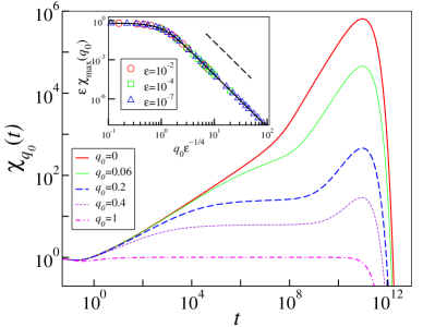
Figure 1: Numerical solution of the schematic IMCT equations for $T>T_{c}$, where all $k$ dependence is neglected (see BBMRlong for details). Main plot: $\chi_{{\bf q}_{0}}(t)$ for different ${\bf q}_{0}$ as a function of time, and for $\varepsilon=10^{-6}$. From top to bottom: $q_{0}=0,0.06,0.2,0.4,1.$. Note that the shape of $\chi_{{\bf q}_{0}}(t)$ in the $\alpha$ regime is independent of ${\bf q}_{0}$, as predicted by Eq. (5). We have in fact checked that the predicted scaling is very well obeyed in that region. Inset: $\varepsilon\chi_{\max}({\bf q}_{0})\equiv\varepsilon\chi_{{\bf q}_{0}}(t=\tau_{\alpha})$ as a function of $q_{0}\varepsilon^{-1/4}$ in log-log, for different $q_{0}$’s and $\varepsilon$’s. Note the $q_{0}^{-4}$ behaviour for large $q_{0}\varepsilon^{-1/4}$, as indicated by the dashed line.

The analysis of $\chi_{{\bf q}_{0}}({\bf k},t)$ in the $\alpha$-relaxation regime turns out to be more subtle than anticipated in BB and will be detailed elsewhere BBMRlong . We have established that for small $q_{0}$ and fixed $\varepsilon$,

$$\chi_{{\bf q}_{0}}({\bf k},t)=\frac{\Xi(\Gamma q_{0}^{2}/\sqrt{\varepsilon})}{\sqrt{\varepsilon}(\sqrt{\varepsilon}+\Gamma q_{0}^{2})}\,g_{\alpha,k}\left(\frac{t}{\tau_{\alpha}}\right),$$ (5)

with $\Xi$ a certain regular function with $\Xi(0)\neq 0$ and $\Xi(v\gg 1)\sim 1/v$ such that $\chi_{{\bf q}_{0}}$ behaves as $q_{0}^{-4}$ for large $q_{0}$, independently of $\varepsilon$. Also, $g_{\alpha,k}(u\ll 1)=S(k)h(k)u^{b}$, as to match the $\beta$ regime, and $g_{\alpha}(u\gg 1,k)\to 0$. All those analytical results are in full agreement with the numerical solution of the schematic version of IMCT equations (see Fig. 1). Note that the scaling variable is still $q_{0}^{2}\varepsilon^{-1/2}$ in that regime, rather than $q_{0}^{2}\varepsilon^{-1}$ as surmised in BB EPL . The physical consequence of the above analysis is the existence of a unique diverging length scale $\xi\sim\sqrt{\Gamma}|\varepsilon|^{-1/4}$ that rules the response of the system to a space-inhomogeneous perturbation and hence of the spatial dynamic correlations. The analysis of the early $\beta$ regime where $t\ll|\varepsilon|^{-1/2a}$ BBMRlong shows that this length in fact first increases as $t^{a/2}$ and then saturates at $\xi$. Furthermore, Eq. (5) indicates that although the integrated dynamic correlation $\chi_{{\bf q}_{0}=0}({\bf k},t)$ increases in the $\alpha$ regime as $\varepsilon^{(b-a)/2a}t^{b}$ (from $\varepsilon^{-1/2}$ for $t=\tau_{\beta}$ to $\varepsilon^{-1}$ for $t=\tau_{\alpha}$) the dynamic length scale itself remains fixed at $\xi$. Interestingly, this suggests that while keeping a fixed extension $\xi$, the (fractal) geometrical structures carrying the dynamic correlations significantly ‘fatten’ ftnfrac between $\tau_{\beta}$ (where the structures could correspond to the strings reported in recent simulations Glotzer ; Heuer ) and $\tau_{\alpha}$, where more compact structures are expected, as indeed suggested by the results of Kob . For $\tau_{\beta}\ll t\ll\tau_{\alpha}$, we expect a cross-over between dense and dilute structures at a new, time dependent crossover length BBMRlong .

Starting from the general IMCT equation Eq. (1), one could have chosen to follow a slightly different path and only assume that the length scale $\ell$ of the imposed inhomogeneities is large, and perform a gradient expansion to order $\ell^{-2}$ to obtain an equation on the space dependent structure factor, $F({\bf q},{\bf r},t)$. This space-dependent Ginzburg-Landau like MCT equation has one part that is identical to standard MCT equation (with space dependent coefficients) plus non linear contributions containing a $\nabla^{2}F$ term and, interestingly, a Burgers non-linear term of the form $(\nabla F)^{2}$ BBMRlong . When inhomogeneities are small, $F({\bf q},{\bf r},t)=F_{0}({\bf q},t)+\chi({\bf q},{\bf r},t)$ with $\chi\ll F_{0}$, these equations become identical to Eq. (2) above. In the schematic limit where all wave-vector dependencies drop off, our equation coincides with the gradient expansion obtained by Franz for the p-spin glass model in the Kac limit Franz .
In summary, we have shown how to extend the standard framework of MCT to inhomogeneous situations. This allows us to compute the response of the dynamical structure factor to spatial perturbations. The case of a localized perturbation at the origin is particularly interesting: it shows directly that the dynamical structure factor is affected on a dynamic length scale $\xi$ that diverges as $|\varepsilon|^{-\nu}$ as the Mode-Coupling transition is approached, with $\nu=1/4$ and a prefactor that can be computed numerically. This length scale governs both the $\beta$ and $\alpha$ relaxation regimes, showing that the standard interpretation of the $\beta$-regime as the vibrations of particles trapped in independent cages formed by nearest neighbors is somewhat misleading: as the MCT transition is approached, $\xi$ grows and the ‘cages’ become more and more collective. Our results suggest an interesting scenario where the geometrical structures responsible for dynamic fluctuations thicken with time. Note that $\xi$, as in ordinary critical phenomena, only diverges at $T_{c}$, reflecting the critical fragility of the system right at the transition. It is therefore clearly distinct from the diverging viscous length $\sqrt{\eta\tau_{\alpha}}$ which sets the scale below which the liquid sustains shear waves Das , which is infinite in the whole glass phase. Our IMCT equations should be very useful to investigate inherently inhomogeneous physical situations. Also, spatial critical fluctuations are expected to play a major role in low dimensions, as for usual critical phenomena. These should lead to non trivial values of critical exponents (such as $\nu$) and be involved in the breakdown of the Stokes-Einstein relation between viscosity and diffusion BBdecoup . However, these critical fluctuations should also interfere with activated ‘droplet’ fluctuations that are expected to smear out the MCT transition in finite dimensions BBChem . The details of the way these two type of phenomena interact and lead to the observed crossover between an MCT-like regime and an activated regime in supercooled liquids is, in our opinion, one of the most crucial open theoretical questions. Mixing the present framework with the extended Mode-Coupling scheme recently proposed in eMCT might be a promising path. Finally, we want to stress that generalized susceptibilities such as $\chi_{{\bf q}_{0}}({\bf k},t)$ offer a direct way to study correlations between dynamics and local structural fluctuations Science . They provide a complementary and more direct physical information than the 4-point correlations studied in Parisilength ; Glotzer ; Berthier . We notice that $\chi_{{\bf q}_{0}}({\bf k},t)$ can be measured using state of the art molecular or Brownian dynamics simulation. Experimentally, it could be accessible in colloids by use of an optical tweezer array imposing a periodic dielectric force on the particles.

We warmly thank L. Berthier, S. Franz, W. Kob, V. Krakoviack, G. Tarjus, M. Wyart and F. Zamponi. GB is partially supported by EU contract HPRN-CT-2202-00307 (DYGLAGEMEM) and DRR by grants NSF CHE-0505939 and NSF DMR-0403997.

References

- (1) M. D. Ediger, Ann. Rev. Phys. Chem. 51, 99 (2000).
- (2) M. Hurley, P. Harrowell, Phys. Rev. E 52, 1694 (1995).
- (3) R. Yamamoto and A. Onuki, Phys. Rev. Lett. 81, 4915 (1998).
- (4) G. Parisi, J. Phys. Chem. B. 103 4128 (1999).
- (5) C. Bennemann, C. Donati, J. Bashnagel, S. C. Glotzer, Nature, 399, 246 (1999), S. C. Glotzer, J. Non-Cryst. Solids 274, 342 (2000), see also FP .
- (6) L. Berthier, Phys. Rev. E 69, 020201 (2004); S. Whitelam, L. Berthier, J.P. Garrahan, Phys. Rev. Lett. 92, 185705 (2004).
- (7) O. Dauchot, G. Marty and G. Biroli, Phys. Rev. Lett. 95 265701 (2005).
- (8) L. Berthier, G. Biroli, J.-P. Bouchaud, L. Cipelletti, D. El Masri, D. L ’Hote, F. Ladieu, M. Pierno, Science 310, 1797 (2005), and BBBKMR
- (9) F. Ritort, P. Sollich, Adv. Phys. 52, 219 (2003).
- (10) J. P. Garrahan, D. Chandler, Phys. Rev. Lett. 89, 035704 (2002).
- (11) W. Götze, L. Sjögren, Rep. Prog. Phys. 55 241 (1992).
- (12) W. Götze, Condensed Matter Physics, 1, 873 (1998).
- (13) T.R. Kirkpatrick and D. Thirumalai, Phys. Rev. A 37, 4439 (1988); T.R. Kirkpatrick, P.G. Wolynes, Phys. Rev. B 36, 8552 (1987)
- (14) S. Franz, G. Parisi, J. Phys.: Condens. Matter 12, 6335 (2000); C. Donati, S. Franz, G. Parisi, S. C. Glotzer, J. Non-Cryst. Sol., 307, 215 (2002).
- (15) see A. Montanari, G. Semerjian, cond-mat/0603018.
- (16) G. Biroli, J.P. Bouchaud, Europhys. Lett. 67, 21 (2004).
- (17) K. Miyazaki, D. R. Reichman, J. Phys. A: Math.Gen. 38, L343 (2005).
- (18) A. Andreanov, G. Biroli, A. Lefèvre, cond-mat/0510669
- (19) M. E. Cates and S. Ramaswamy, Phys. Rev. Lett. 96, 135701 (2006).
- (20) G. Biroli, J. P. Bouchaud, in preparation.
- (21) see V. Krakoviack, Phys. Rev. Lett. 94 065703 (2005) for MCT in pores, but for averaged quantities for which explicit inhomogeneities have disappeared.
- (22) P. Scheidler, W. Kob, K. Binder, J. Phys. Chem. B, 108, 6673 (2004)
- (23) D. R. Reichman and P. Charbonneau, J. Stat. Mech. P05013 (2005).
- (24) G. Biroli, J.-P. Bouchaud, K. Miyazaki, D. R. Reichman, in preparation.
- (25) L. Berthier, G. Biroli, J.-P. Bouchaud, W. Kob, K. Miyazaki, D. R. Reichman, forthcoming.
- (26) W. Götze, Z. Phys. B 60, 195 (1985)
- (27) This modulated glass bears some resemblance with, but is different from, the stripe glass of J. Schmalian, P. G. Wolynes, Phys. Rev. Lett. 85, 836 (2000).
- (28) Our results suggest that in high dimensions, the fractal dimension of the dynamic clusters increases from in the regime to in the regime.
- (29) M. Vogel, B. Doliwa, A. Heuer, S.C. Glotzer, J. Chem. Phys. 120, 4404 (2004).
- (30) G. A. Appignanesi, J. A. Rodriguez Fris, R. A. Montani, and W. Kob, Phys. Rev. Lett. 96, 057801 (2006)
- (31) S. Franz and F. L. Toninelli, J. Phys. A: Math. Gen. 37 (2004) 7433 and private communication.
- (32) R. Ahluwalia, S. P. Das, Phys. Rev. E 57, 5771 (1998).
- (33) T. R. Kirkpatrick, D. Thirumalai, P. G. Wolynes, Phys. Rev. A, 40 (1989) 1045; J. P. Bouchaud and G. Biroli, J. Chem. Phys. 121, 7347 (2004).
- (34) P. Mayer, K. Miyazaki, D. R. Reichman, cond-mat/0602248.