Stochastic Green’s function approach to disordered systems

Abstract

Based on distributions of local Green’s functions we present a stochastic approach to disordered systems. Specifically we address Anderson localisation and cluster effects in binary alloys. Taking Anderson localisation of Holstein polarons as an example we discuss how this stochastic approach can be used for the investigation of interacting disordered systems.

1 Introduction

In many cases the influence of crystal imperfections present in any real material can be neglected in favour of the interactions dominating e.g. electron transport or optical properties. In some cases however, and especially at low temperatures, interesting physical effects arise from the specific physical processes induced by scattering on crystal defects. Examples range from the quantum Hall effect – an intricate problem far beyond the scope of our study – to electrical transport in polaronic systems. One prominent example is Anderson’s prediction that in a disordered material itinerant (extended) states can be turned into localised states which do not carry any current [1]. This transition from extended to localised states is a result of quantum interference arising from elastic scattering on impurities in a crystal. It leads, roughly speaking, to spatial confinement of an electron: The electron wave-function decays exponentially with distance.

This peculiar, essentially quantum mechanical behaviour has motivated lots of research (see e.g. [2] for a review). As yet, however, many important questions in the field of localisation physics have not been finally settled, and localisation in interacting systems is still far from being understood. Progress on this topic requires new techniques which allow for a comprehensive – necessarily approximate, but reliable – description of disorder and interaction on a microscopic scale. One possible approach shall be discussed here.

The focus of our study is on substitutionally disordered three-dimensional materials like doped semiconductors or alloys. We will not be concerned with amorphous materials like glasses which do not possess a crystal lattice (but see e.g. [3, 4]). Then disorder primarily manifests through site-dependent local potentials $\epsilon_{i}$. The motion of an electron in such a disordered crystal is described by the tight-binding Hamiltonian

$$H=\sum_{i}\epsilon_{i}c^{\dagger}_{i}c_{i}-t\sum_{\langle i,j\rangle}c^{\dagger}_{i}c_{j}\;.$$ (1)

In a perfect crystal, i.e. $\epsilon_{i}=0$, the electron hopping $t$ between nearest–neighbour sites $\langle i,j\rangle$ gives rise to a band of width $W_{0}$, e.g. on a cubic lattice $W_{0}=12t$, or $W_{0}=4t\sqrt{K}$ on a Bethe lattice with connectivity $K$. In what follows, we fix the bandwidth $W_{0}=1$, and measure energies in units of $W_{0}$.

To model the stochastic character of disorder the $\epsilon_{i}$ are considered as random variables with a given distribution. We demand that they are independently identically distributed with common distribution $P(\epsilon_{i})$. For such a stochastic Hamiltonian quantities like the (retarded) Green’s function $G_{ij}(\omega)=\lim_{\eta\to 0^{+}}\langle 0|c_{i}\left[\omega+\mathrm{i}\eta-H\right]^{-1}c^{\dagger}_{j}|0\rangle$ are random variables in their own right. It is thus reasonable to ask for their distributions. This is especially true for the local density of states (LDOS)

$$\rho_{i}(\omega)=-\mathrm{Im}\;G_{ii}(\omega)/\pi\;.$$ (2)

Its distribution $P[\rho_{i}(\omega)]$ gives the statistics of the LDOS in a disordered system, where translational symmetry is broken and $\rho_{i}(\omega)$ varies with $i$. Note that $P[\rho_{i}(\omega)]$ does not depend on the site index $i$: Translational symmetry is restored on the level of distributions. It is important to realise that the site-dependence of the LDOS constitutes an eminent aspect of a disordered system. For an extended state, for example, $\rho_{i}(\omega)$ has a finite value on most lattice sites. For a localised state, in contrast, $\rho_{i}(\omega)$ has exponentially small values on lattice sites outside a finite region, corresponding to the decay of the wave-function. $P[\rho_{i}(\omega)]$ will thus be different for extended and localised states. Obviously the disorder averaged density of states (DOS)

$$\rho_{\mathrm{ave}}(\omega)=\langle\rho_{i}(\omega)\rangle=\int\limits_{0}^{\infty}\rho_{i}\;P[\rho_{i}(\omega)]\;d\rho_{i}\;,$$ (3)

merely counting the number of states at a given energy $\omega$, cannot account for this signature. Only for the ordered case $P(\epsilon_{i})=\delta(\epsilon_{i})$, when translational symmetry implies that $\rho_{i}$ does not depend on $i$, the distribution is entirely determined by the DOS, $P[\rho_{i}(\omega)]=\delta[\rho_{i}-\rho_{\mathrm{ave}}(\omega)]$. As we will later see a similar characterisation does not even hold approximatively in a disordered system. The full distribution can be extremely broad for states in which the electron strongly scatters at impurities, catching the resulting deviations in $\rho_{i}$.

2 Local distribution approach

Our goal is to obtain a calculational scheme for the distribution of the LDOS for the models given by Eq. (1). This scheme must account for the correlations that make up Anderson localisation. At the same time it should be extendable to incorporate interactions. Naturally this requires to employ approximations. It is important to guarantee that within these approximations the mutual influence of interaction and disorder at the microscopic scale is still represented (which rules out e.g. the coherent potential approximation (CPA), see below). A definite candidate to meet these demands is what we call the local distribution (LD) approach. It provides a self-consistent scheme for the distribution $P[G_{ii}(\omega)]$ of the local Green’s function $G_{ii}(\omega)$. We first describe this approach and its application to disordered systems, and later will combine it with a treatment of interaction.

2.1 LD approach on a Bethe lattice

It is straightforward to construct the LD approach following the work of Abou-Chacra, Anderson and Thouless [5]. We briefly repeat their derivation which is carried out on a Bethe lattice (see Fig. 1). The basic observation is the decomposition of the local Green’s function $G_{ii}(\omega)$,

$$G_{ii}(\omega)=\left[\omega-\epsilon_{i}-t^{2}\sum_{j=1}^{K}G^{(i)}_{jj}(\omega)\right]^{-1}\;.$$ (4)

The sum runs over the $K$ neighbours $j$ of $i$, and the Green’s functions $G^{(i)}_{jj}(\omega)$ have to be calculated for the lattice after site $i$ is removed. For the ordered case we have $G^{(i)}_{jj}=G_{ii}(\omega)$ (cf. Fig 1), and Eq. (4) is a quadratic equation for the Green’s function. Especially we can read off the semi-circular DOS $\rho(\omega)=4/(\pi W_{0}^{2})\sqrt{W_{0}^{2}-4\omega^{2}}$ of the Bethe lattice [6].

Now the stochastic viewpoint comes into play. For a disordered system, like $\epsilon_{i}$ all Green’s functions are stochastic quantities, i.e. random variables, and Eq. (4) determines the random variable $G_{ii}(\omega)$ in terms of $K+1$ others, namely $\epsilon_{i}$ and $G^{(i)}_{jj}(\omega)$. On the Bethe lattice the Green’s functions $G^{(i)}_{jj}(\omega)$ correspond to the same geometrical situation as $G_{ii}(\omega)$, hence they are identically distributed. Furthermore no path connects the sites $j=1,\dots,K$ if $i$ is removed. This implies that the $G^{(i)}_{jj}(\omega)$ are independently distributed. Therefore Eq. (4) can be regarded as a self-consistency equation which determines the distribution of one random variable, the local Green’s function $G_{ii}(\omega)$, or equivalently $G^{(i)}_{jj}(\omega)$. The distribution $P(\epsilon_{i})$ enters this equation as a parameter.

Such a stochastic self-consistency equation can be numerically solved by a Monte-Carlo procedure (Gibbs-sampling). To this end we represent the random variable $G_{ii}(\omega)$ through a sample of $N$ entries (typically $N=10^{4}\dots 10^{7}$). Each entry of the sample is repeatedly updated by a new value from Eq. (4), with $K$ values for $G^{(i)}_{jj}(\omega)$ randomly drawn from the sample and a randomly chosen $\epsilon_{i}$. The distribution of $G_{ii}(\omega)$ is finally constructed like a histogram by counting the number of entries in the sample with a specific value.

Figure 1: Sketch of the (half-infinite) Bethe lattice with coordination number $K=2$. When site $i$ is removed from the lattice the sites $j$ are in the same geometrical situation as site $i$ before, and no path connects them.

2.2 LD approach on arbitrary lattices

To put the LD approach in a more general context we will show how to construct it as an approximative scheme on others than the Bethe lattice, thereby making contact to the CPA (concerning CPA see e.g. [7]). On an arbitrary lattice the Green’s function can still be decomposed as

$$G_{ii}(\omega)=\left[\omega-\epsilon_{i}-t^{2}\sum_{l,j=1}^{K}G^{(i)}_{lj}(\omega)\right]^{-1}\;.$$ (5)

In contrast to the Bethe lattice the $G^{(i)}_{lj}(\omega)$ which appear in this decomposition do not correspond to the same geometrical situation as $G_{ii}(\omega)$. If we iterated Eq. (5) we would thus end up with an infinite hierarchy of equations containing many different Green’s functions. As an immediate consequence the LD approach, relying on local Green’s functions, will provide only an approximative scheme on general lattices.

A simple approximation is suggested by introducing

$$H^{(i)}_{j}(\omega)=t^{2}\sum_{l=1}^{K}G^{(i)}_{lj}(\omega)$$ (6)

which is the part of the $K$ hopping contributions in Eq. (5) where the electron leaves site $i$ through $j$. Specifically we assume that, for each $j$, $H^{(i)}_{j}(\omega)$ is determined by the local Green’s function $G_{jj}(\omega)$ alone. Moreover, the $K$ Green’s functions $G_{jj}(\omega)$ are taken to be independently distributed.

To proceed further we write the local Green’s function with a self-energy like in the CPA

$$G_{ii}(\omega)=G^{0}(\omega-\Sigma_{i}(\omega))\;,$$ (7)

where $G^{0}(\omega)$ is the ‘bare’ propagator for the ordered system. In contrast to the CPA the self-energy $\Sigma_{i}(\omega)$ is now site-dependent. Thinking in terms of an effective medium in which site $i$ is embedded this medium is characterised by the distribution of self-energies $\Sigma_{i}(\omega)$. The electron at site $i$ ‘sees’ the effective medium through the $K$ Green’s functions $G_{jj}(\omega)$. Being part of the effective medium the hybridisation $H^{(i)}_{j}(\omega)$ associated with $G_{jj}(\omega)$ must fulfil $G_{jj}(\omega)=\left[\omega-\Sigma_{j}-KH^{(i)}_{j}(\omega)\right]^{-1}$. Inverting this equation yields

$$H^{(i)}_{j}(\omega)=\frac{1}{K}\left(\omega-\Sigma_{j}-\left[G_{jj}(\omega)\right]^{-1}\right)\;.$$ (8)

The Green’s function $G_{ii}(\omega)$ is then given by $K$ other Green’s function $G_{jj}(\omega)$ of the same type:

$$G_{ii}(\omega)=\left[\omega-\epsilon_{i}-\sum_{j=1}^{K}H^{(i)}_{j}(\omega)\right]^{-1}=\left[\frac{1}{K}\sum_{j=1}^{K}\left[G_{jj}(\omega)\right]^{-1}-\epsilon_{i}+\frac{1}{K}\sum_{j=1}^{K}\Sigma_{j}(\omega)\right]^{-1}\;.$$ (9)

Clearly, if all $\epsilon_{i}=0$, this equation reduces to $\Sigma_{i}=0$, that is $G_{ii}(\omega)=G^{0}_{ii}(\omega)$.

At last, we have a complete set of equations, which with the same Monte-Carlo-scheme as before can be solved to determine the distribution of $G_{ii}(\omega)$. Note that the approximations we made are guaranteed to respect causality, in the sense that $\mathrm{Im}\,G_{ii}(\omega),\,\mathrm{Im}\,\Sigma_{i}(\omega)<0$. Eqs. (7) and  (9) are immediately seen to preserve this important property. For Eq. (8), where this property is not obvious, we can rely on a result from the analyticity proof of the CPA [8], which states that $\mathrm{Im}\left\{\Sigma+\left[G^{0}(\omega-\Sigma)\right]^{-1}\right\}>0$ for $\mathrm{Im}\,\Sigma<0$.

We like to point out that the construction done here is slightly ambiguous. A different approximation in Eq. (8) would still give a self-consistent scheme for distributions of local Green’s functions $G_{ii}(\omega)$. Anyhow, our scheme incorporates the CPA and reproduces the exact scheme for the Bethe lattice in a natural way. The CPA results from Eq. (9) for $K=\infty$ by the central limit theorem. Then, the sums over Green’s functions and self-energies are replaced by averages, yielding the CPA equation for the averaged local Green’s function

$$G^{\mathrm{CPA}}(\omega)=\left\langle\frac{1}{\left[G^{\mathrm{CPA}}(\omega)\right]^{-1}-(\epsilon_{i}-\Sigma(\omega))}\right\rangle\;.$$ (10)

In principle, $K$ is in our scheme no free parameter but the number of neighbours to a lattice site. If we increase $K$ the bare propagator $G^{0}(\omega)$ changes, and therefore we shall scale $t$ as $t\propto 1/\sqrt{K}$ like in the limit of high dimension [9]. Then, for $K\to\infty$, our scheme still reduces to the CPA, which is known to become exact for lattices with infinite connectivity [10]. This implies that the approximations we made are good for high-dimensional lattices. Actually they turn out to be good for $d\geq 3$. It is commonly known that CPA is the best single-site approximation for disordered systems. The local Green’s function is obtained on average from an ‘averaged’ effective medium. The LD approach solves the local problem exactly, while the hybridisation is calculated from a ‘fluctuating’ effective medium. So to say, the LD approach is the best single-site approximation if fluctuations are taken into account.

On the Bethe lattice the Green’s function fulfils $G^{0}_{ii}(\omega)=\left[\omega-t^{2}KG^{0}_{ii}(\omega)\right]^{-1}$ (this is just Eq. (4) for $\epsilon_{i}=0$), whereby Eq. (7) reads

$$\Sigma_{i}(\omega)-\left[G_{ii}(\omega)\right]^{-1}=\omega-t^{2}KG_{ii}(\omega)$$ (11)

Then Eq. (9) reduces to Eq. (4) for the Bethe lattice. The key point is of course that, owing to the specific Bethe lattice geometry, the non-diagonal contributions $G^{(i)}_{jl}$ are zero, and the $H^{(i)}_{j}$ are indeed independently distributed. Then our approximation scheme becomes exact: On the Bethe lattice the best single-site approximation, with fluctuations, is an exact theory. Note that for the Bethe lattice $K$ is a free parameter: The ‘free’ DOS in absence of disorder is, for fixed $W_{0}$, independent of $K$, but choosing $K$ fixes the Bethe lattice used.

As the transfer of the LD approach to other lattices shows, going to the Bethe lattice basically changes the ‘free’ DOS and introduces approximations to cubic lattices by neglecting correlations. The essential properties of disordered systems, e.g. localisation, will however be well described. For the time being we work on a $K=2$ Bethe lattice.

3 Disordered crystals

Below we will discuss two models, the Anderson model with a ‘continuous’ probability distribution, and the binary alloy model with a ‘discrete’ one. While the former is dominated by the Anderson transition from extended to localised states, the latter is dominated by multiple electron scattering on clusters of atoms, visible e.g. in the fragmentation of the DOS (see below).

3.1 Anderson model

In the Anderson model, with disorder strength $\gamma\geq 0$, the $\epsilon_{i}$ have a box distribution

$$P(\epsilon_{i})=(1/\gamma)\,\Theta(\gamma/2-|\epsilon_{i}|)\;.$$ (12)

Figure 2: Change of the probability distribution $P[\rho_{i}(\omega)]$ of the LDOS $\rho_{i}(\omega)$ for the Anderson model, in the band centre $\omega=0$, with increasing $\gamma$. Note that the inset has a logarithmic $\rho_{i}$-axes.

Fig. 2 shows the change of the distribution $P[\rho_{i}(\omega)]$ of the LDOS with increasing disorder, as obtained from our Monte-Carlo scheme. We find the behaviour indicated in the introduction. For small disorder the distribution is rather Gaussian, but becomes strongly asymmetric and extremely broad as $\gamma$ increases. The (averaged) DOS $\rho_{\mathrm{ave}}(\omega)$ is not indicative of these distributions. If $\gamma$ exceeds a critical value $\gamma_{c}(\omega)$ [$\gamma_{c}(\omega=0)\simeq 3.0$] the distribution becomes singular while $\rho_{\mathrm{ave}}(\omega)$ is still finite. At this point the transition from extended to localised states takes place. To determine $\gamma_{c}(\omega)$ numerically we have to study the scaling of appropriate quantities, like for any phase transition. Here we employ the different behaviour of $P[\rho_{i}(\omega)]$ when the imaginary part $\eta$ in the energy argument of $G_{ii}(\omega+\mathrm{i}\eta)$ goes to zero: For extended (localised) states the distribution is stable (instable) for $\eta\to 0$ (see Fig. 3). This behaviour is again not caught by $\rho_{\mathrm{ave}}(\omega)$, which is finite for $\eta\to 0$ for both extended and localised states. But suitable moments of the distribution, like the geometric average, drop to zero just for localised states (see inset in Fig. 3). With this criterion which numerically tests whether the distribution is singular or not we can very precisely distinguish extended and localised states [11]. Fig. 4 shows the phase diagram of the Anderson model on the Bethe lattice obtained by means of the limit $\eta\to 0$. It displays two important features of localisation. First, the existence of a critical disorder $\gamma_{c}(\omega=0)$ above which all states are localised due to the strong impurity scattering. Second, before complete localisation occurs, states towards the band centre are extended while states towards the band edges are localised, these states being separated by the so-called mobility edges. Furthermore the mobility edge trajectory reveals that for small disorder the electron tunnels between impurities, giving rise to extended states outside the band $[-W_{0}/2,W_{0}/2]$ of the ordered system.

Let us finally contrast the LD result for $\rho_{\mathrm{ave}}(\omega)$ (Fig. 4) with the CPA. The CPA reproduces the DOS very good inside the band – only here $P[\rho_{i}(\omega)]$ is a Gaussian – but fails closer to the band edges where it misses the (Lifshitz) tails in the DOS. These tails result from states at the band edges which come along with repeated scattering of the electron on clusters of impurities with a large (or small) potential $\epsilon_{i}$. Since multi-scattering is not accounted for in the CPA these states cannot be described.

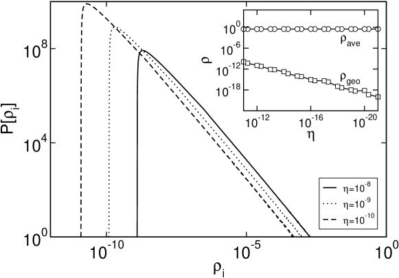
Figure 3: The figure displays, for localised states ($\gamma=1.5$, $\omega=0.9$), the change of $P[\rho_{i}]$ with decreasing $\eta$. The inset shows that $\rho_{\mathrm{ave}}$ is constant for $\eta\to 0$, but a typical moment, the geometrically averaged DOS $\rho_{\mathrm{geo}}=\exp\langle\ln\rho_{i}\rangle$, goes to zero. For extended states we get distributions like in Fig. 2, independent of (a small) $\eta$.

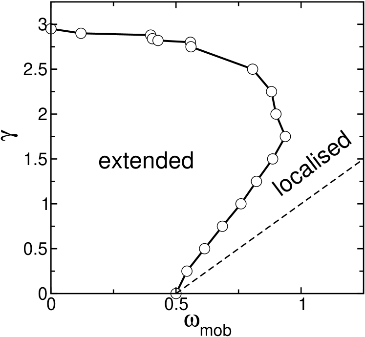
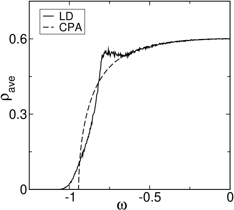
Figure 4: Left panel: Mobility edge trajectory, i.e. the phase diagram, of the Anderson model, obtained in the limit $\eta\to 0$. The dashed lines indicate the band edges $\pm(W/2+\gamma/2)$. Right panel: DOS for the Anderson model at $\gamma=1.5$ for $\omega\leq 0$, calculated with CPA and LD approach. Both the DOS and the phase diagram are symmetric under $\omega\to-\omega$.

3.2 Binary alloy

Multi-scattering becomes rather important for ‘discrete’ distributions like

$$P(\epsilon_{i})=c_{A}\delta(\epsilon_{i}+\Delta/2)+(1-c_{A})\delta(\epsilon_{i}-\Delta/2)\,,$$ (13)

describing a two-component binary alloy made of ‘A-atoms’ with potential $-\Delta/2$ and ‘B-atoms’ with potential $+\Delta/2$. Thus we have two parameters, the concentration $c_{A}$ of the A-species and the energy separation $\Delta$.

Exemplarily we consider the case $c_{A}=0.1$ when the A-atoms form the minority species in a bulk of B-atoms, and $\Delta=2.0$ when the A-atoms are energetically well-separated from the band of the B-bulk. Fig. 5 shows the corresponding DOS, contrasting the LD and CPA results. The B-band is rather smooth and almost reproduced by the CPA, which nevertheless misses important features. In the energy range of the A-atoms we do not find a band but a strongly fragmented set of peaks. Each of these peaks can be attributed to a specific cluster of A-atoms, as indicated in the figure. Due to the low concentration $c_{A}$ of A-atoms, and the large energy separation $\Delta$, states at these clusters do not hybridise and form a continuous band, but are essentially confined to the clusters and contribute discrete peaks to the DOS. The CPA is by construction unable to identify those cluster states and therefore entirely misses band fragmentation. With increasing $\Delta$ these signatures become more prominent, while CPA suggests that the bands, being well separated, less influence each other (see right panel in Fig. 5). The CPA is of course able to depict gross features as band splitting, but replaces the complex spectrum by semi-circular bands with weight $c_{A}$ and $1-c_{A}$. Then, e.g., the minority A-band has spectral weight outside the CPA band: Replacing this band by a semi-circular one while conserving the overall spectral weight $c_{A}$ results in a clearly reduced CPA bandwidth.

We think that the binary alloy is a particular instructive example how, using the distribution of $G_{ii}(\omega)$, one manages to account for multi-scattering events which are absent in a CPA description relying on averaged values. With a proper treatment of multi-scattering like in the LD approach both quantum interference leading to Anderson localisation and formation of cluster states is correctly described.

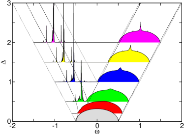
Figure 5: Left panel: DOS for the binary alloy model at $\Delta=2.0$, $c_{A}=0.1$, contrasting the CPA and LD results. Arrows mark different peaks in the DOS which arise from the clusters indicated (e.g. A-BB indicates the contribution from an A-atom which is surrounded by two B-atoms.) We used in the figure an arbitrary $\eta=10^{-3}$ to broaden the peaks. Right panel: Kind of a phase diagram for the binary alloy model at $c_{A}=0.1$, showing the DOS for various $\Delta$. The dashed curves show the CPA band edges, and the dotted lines mark $\omega=\pm\Delta/2\pm W_{0}/2$ (figures taken from [12])

.

4 Electron-Phonon Coupling

Anderson localisation arises from elastic electron-impurity scattering. Coherence which is maintained during elastic scattering is the important precondition for localisation. To understand which role localisation plays in a real solid we must therefore understand how it is affected by inelastic scattering, which naturally arises from the interaction of the electron with lattice vibrations, i.e. phonons. A model to study the competition between localisation –related to coherence– and electron-phonon (EP) interaction –related to incoherence– is provided by the Anderson-Holstein Hamiltonian

$$H=\sum\limits_{i}\epsilon_{i}c^{\dagger}_{i}c_{i}-t\sum\limits_{\langle i,j\rangle}c_{i}^{\dagger}c_{j}-\sqrt{\varepsilon_{p}\omega_{0}}\sum\limits_{i}(b_{i}^{\dagger}+b_{i})c^{\dagger}_{i}c_{i}+\omega_{0}\sum\limits_{i}b_{i}^{\dagger}b_{i}~{},$$ (14)

which adds a Holstein-type of interaction to the Anderson model, the $\epsilon_{i}$ being distributed according to Eq. (12). Here $b_{i}^{(\dagger)}$ denote bosonic operators describing dispersionless optical phonons with frequency $\omega_{0}$ which are locally coupled to the electron density $c_{i}^{\dagger}c_{i}$. We introduce the dimensionless phonon frequency $\tilde{\omega}_{0}=\omega_{0}/W_{0}$, and a coupling constant $\tilde{\lambda}=2\varepsilon_{p}/W_{0}$. Moreover we consider one electron at $T=0$.

Besides introducing incoherent motion, EP coupling in this model can lead to the formation of a new quasiparticle. Sufficiently strong EP coupling binds the electron to the lattice deformation at the electron’s site, forming a new compound entity, the polaron (see e.g. [13]). A polaron is strongly mass-enhanced and therefore very much affected by disorder. However, a polaron is not just a heavy electron. Due to inelastic scattering and retardation of the EP interaction in most cases the internal structure of the polaron will play a crucial role, leading to different localisation properties. Moreover if inelastic scattering dominates, leading to incoherent motion of the polaron, localisation will be suppressed. Then a polaron can be less easy to localise than the free electron, although its mass is still increased.

4.1 Extending the LD approach to interacting systems

Like in the standard Green’s functions formalism interaction is incorporated in the LD approach by an interaction self-energy $\Sigma^{I}_{ij}(\omega)$ [14]. The ‘disorder’ self-energy $\Sigma_{i}$, as introduced in Eq. (7), is local. The interaction self-energy will be approximated to be local as well. The Green’s function $G_{ii}(\omega)$ is then obtained as

$$G_{ii}(\omega)\!=\!\left[\omega-\epsilon_{i}-\Sigma^{I}_{i}(\omega)-\sum_{j=1}^{K}H^{(i)}_{j}(\omega)\right]^{-1}\!=\!\left[\frac{1}{K}\sum_{j=1}^{K}\left[G_{jj}(\omega)\right]^{-1}-\epsilon_{i}-\Sigma^{I}_{i}(\omega)+\frac{1}{K}\sum_{j=1}^{K}\Sigma_{j}(\omega)\right]^{-1}\!\!\!,$$ (15)

replacing Eq. (9). Like for the disorder part one should demand [15] that the interaction self-energy is obtained as the ‘best’ local self-energy which amounts to use the dynamical mean field theory (DMFT) (for a review see [16]). Within DMFT the interaction self-energy is a functional $\Sigma^{I}_{i}(\omega)=\Sigma^{I}_{i}[F_{i}(\omega)]$ of the local propagator

$$F_{i}(\omega)=\left[\omega-\epsilon_{i}-\sum_{j=1}^{K}H^{(i)}_{j}(\omega)\right]^{-1}$$ (16)

which does not contain $\Sigma^{I}_{i}(\omega)$. With the DMFT self-energy inserted into the equations still the Monte-Carlo scheme applies. Since the interaction couples different energies each entry of the sample now represents a local Green’s function $G_{ii}(\omega)$ on a set of $\omega$ (e.g. Matsubara frequencies). Note that during each update of an entry one has to evaluate $\Sigma^{I}_{i}[F_{i}(\omega)]$. Without disorder, for $\epsilon_{i}=0$, this scheme reduces to standard DMFT.

The functional dependence $\Sigma^{I}_{i}[F_{i}(\omega)]$ is not explicitly known but requires, despite the approximations made, the solution of a quantum-mechanical many-particle problem. Solving this model constitutes the main part of a DMFT implementation. Concerning disordered interacting system the evolved calculation of $\Sigma^{I}_{i}[F_{i}(\omega)]$ poses a severe problem. So far system with a finite charge carrier density like a disordered Hubbard model could only be addressed in limiting cases [15]. For a single electron in the Anderson-Holstein model we are fortunate to explicitly know the functional $\Sigma^{I}_{i}\left[F_{i}(\omega)\right]$, given as an infinite continued fraction for $T=0$ [17, 18]:

$$\Sigma^{I}_{i}(\omega)=\frac{\displaystyle 1\varepsilon_{p}\omega_{0}}{\displaystyle\left[F_{i}(\omega-1\omega_{0})\right]^{-1}-\frac{\displaystyle 2\varepsilon_{p}\omega_{0}}{\displaystyle\left[F_{i}(\omega-2\omega_{0})\right]^{-1}-\frac{\displaystyle 3\varepsilon_{p}\omega_{0}}{\displaystyle\cdots}}}\,.$$ (17)

The $p$-th level of this continued fraction corresponds to the emission of $p$ virtual phonons, shifting the energy argument of $F_{i}$ by $p\omega_{0}$. Originally this expression has been obtained as an extension of the CPA to describe dynamical interaction effects (concerning dynamical CPA, see [17]). In the spirit of the CPA the interaction can be mapped onto an effective Hamiltonian which is related to the original problem via a consistency condition on the Green’s function [19]. This mapping can be combined with the LD construction on the Bethe lattice whereby the consequences of the approximations concerning interaction and disorder become very explicit [11]. It turns out that the interaction induced correlations between local Green’s functions are almost treated on the same level of correctness as the disorder induced correlations. In particular one finds that the extended LD approach comprises cooperative effects which arise from the mutual interplay between interaction and disorder. This is why the LD approach excels approaches which try to replace the interacting disordered system by an effective non-interacting disordered system. The interaction is there mimicked by effective transfer integrals or local potentials, but the feedback of disorder on interaction is not accounted for. The same objection applies if the interacting disordered system is replaced by an effective interacting system, mimicking disorder by effective coupling constants. The price to be paid on using the LD approach is the rather involved numerical implementation combining a repeated solution of the DMFT problem with a Monte-Carlo scheme.

4.2 Polaron localisation

Within the extended scheme just described we can study how the electron is affected by disorder and EP interaction. We will only touch on this question and focus on two significant cases where we compare parts of a phase diagram for polaron localisation to that of the Anderson model. The reader should be aware that we encounter a very complicated physical situation. Already without disorder the Holstein EP interaction displays rich, and very distinct, physics in different parameter regimes. With disorder, cooperative effects like the formation of polaron defect states, come into play. These effects do hardly fit into a ‘universal’ phase diagram of polaron localisation but demand a more concrete description, depending on the specific case studied. A more detailed discussion of this and related issues can be found in [20].

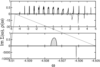
Figure 6: DOS $\rho(\omega)$ without disorder ($\gamma=0$), obtained within DMFT. $\mbox{Im}\,\Sigma(\omega)$ is displayed downwards. Left panel: The strong-coupling, large phonon-frequency case $\tilde{\lambda}=9.0,\,\tilde{\omega}_{0}=0.5625$ can be understood from the atomic limit (independent boson model), treating $t$ as a perturbation. The DOS shows narrow bands which are separated by $\omega_{0}$. The bandwidth of the lowest band (magnified in the bottom row) is $W/W_{0}=3.45\times 10^{-4}$, i.e. the polaron being extremely heavy. Right panel: For weak coupling ($\tilde{\omega}_{0}=0.05$, $\tilde{\lambda}=0.25$, upper row) EP interaction essentially leads to inelastic motion of the electron ($\mathrm{Im}\,\Sigma(\omega)<0$). For stronger coupling ($\tilde{\lambda}=1.0$, same $\tilde{\omega}_{0}=0.05$) a polaron has formed. The lowest polaron band ($W/W_{0}=8.123\times 10^{-3}$) is asymmetric revealing the different character of the polaron to the lower and upper band edge.

In Fig. 6 the DOS for two choices of polaron parameters as obtained by DMFT is shown. We used the $\eta\to 0$ – criterion to obtain the mobility edges for the lowest polaron sub-band in each of the two cases. The comparison to the mobility edges of the Anderson model (Fig. 7) demonstrates that only in special cases the localisation properties of the polaron can be understood as the mere result of the mass renormalisation of the quasiparticle.

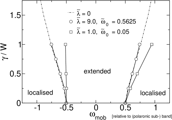
Figure 7: In addition to the phase diagram of the Anderson model the mobility edges for the two polaron bands from Fig. 6 are shown. The mobility edges are drawn relative to the sub-band position, and disorder is measured in units of the sub-band width $W$ [20].

For strong-coupling and large phonon-frequency $\tilde{\lambda}=9.0,\,\tilde{\omega}_{0}=0.5625$ (circles in Fig. 7), the polaron in the lowest band is basically a heavy particle which moves fully coherent but within an extremely narrow band. It localises like a bare electron with a rescaled bandwidth, and the internal structure of the polaron does not play a role. Due to the strong coupling the relevant energy scale for localisation has however changed by four orders of magnitude, making the polaron extremely susceptible to disorder.

For intermediate coupling and small phonon-frequency $\tilde{\lambda}=1.0$, $\tilde{\omega}_{0}=0.05$ (squares in Fig. 7), the polaron motion is, already without disorder, different at the lower and upper band edge. At the lower band edge the polaron is rather mobile, while at the upper band edge it tends to be immobile. Concerning the localisation properties the polaron at the lower band edge is thus almost unaffected by disorder and does not readily localise. At the upper band edge, in contrast, it is easily localised. Note that the lowest polaron band is again coherent: localisation is not just affected by incoherent motion but intricately depends on the internal structure of the polaron. Be also aware that disorder is measured in units of the renormalised band width: the polaron at the lower band edge is more difficult to localise than a bare electron only with respect to the relevant energy scale $W$, i.e. the polaronic bandwidth.

In Fig. 7 we have only shown data for moderate disorder, i.e. below $\gamma_{c}(\omega=0)$ when, for the bare electron, all states become localised. In the first (strong-coupling) case we can indeed localise all states in the lowest polaron band and obtain the respective $\gamma_{c}(\omega=0)$ which has the value of the bare electron renormalised by $W/W_{0}$. Here disorder induced mixing with excited polaron states is prevented by the large gap to the next band ($W\ll\omega_{0}$). In the second (adiabatic intermediate-coupling) case, however, with increasing disorder the lowest band merges with the next polaron band before it is completely localised. Then the relevant energy scale for $\gamma$ changes by one order of magnitude to the joint bandwidths of the two lowest bands. Hence an equivalent to $\gamma_{c}(\omega=0)$ does not exist. Apparently we can only draw parts of a phase diagram for polaron localisation. Again, EP interaction changes the localisation properties in a more complicated way than thinking only in terms of mass renormalisation would suggest.

5 Summary

In disordered systems Green’s functions emerge as stochastic, random quantities. It is reasonable to take this stochastic character serious and to incorporate distributions of those quantities in a description of disorder. Following [5] the proposed LD approach is based on distributions of the local Green’s function. Being exact on a Bethe lattice, approximate on general lattices, it accounts for quantum interference leading to Anderson localisation, and multiple scattering on clusters like in a binary alloy.

The LD approach is an extension of the CPA including fluctuations. Conversely, it contains the CPA in the limiting case when fluctuations are replaced by averages. We can then understand that the CPA results are good if – and only if – the distribution of the LDOS is characterised by its average. This condition does not mean that the disorder is weak: Even for small $\gamma$ in the Anderson model states at the band edges are localised, and beyond the scope of the CPA. A similar restriction exists for the minority band in the binary alloy model.

The great challenge is however not disordered, but interacting disordered systems. Here the LD approach can provide a description of the microscopic interplay between interaction and impurity scattering. Locally, both interaction and impurity scattering are treated in the best approximation possible: DMFT is the best single-site approximation to interaction; and impurity scattering is exactly treated (on general lattices at least locally exact).

The LD approach depends on the accuracy of the DMFT self-energy. A deep understanding of this part of the problem is important. How the involved numerical methods (quantum Monte-Carlo, exact diagonalisation, density matrix renormalisation group, to mention a few) or approximative schemes (e.g. iterative perturbation theory (IPT)) used for the calculation of the DMFT self-energy [16] cope with the considerable fluctuations in the local propagator $F_{i}(\omega)$ induced by disorder is by no means clear (e.g. the perturbative expansion in the IPT is best for weakly varying $F_{i}(\omega)$). Since we largely understand the LD approach’s application to disorder, how to guarantee for the quality of these methods is still the biggest problem – the computational costs for their implementation in the Monte-Carlo scheme notwithstanding. Our results for the localisation of a single Holstein polaron, where these objections are absent, demonstrate that the LD approach by itself allows for a comprehensive description and detailed study of interacting disordered systems. Physically we learned how intricate and rich the interplay of interaction and localisation can be. Future work will certainly support and extend this observation.

We would like to thank F. X. Bronold for valuable discussions.

References

References

- [1] Anderson P W 1958 Phys. Rev. 109(5) 1492
- [2] Kramer B and MacKinnon A 1993 Rep. Prog. Phys. 56 1469–1564
- [3] Logan D E and Wolynes P G 1984 Phys. Rev. B 29 6560
- [4] Logan D E and Wolynes P G 1987 Phys. Rev. B 36 4135
- [5] Abou-Chacra R, Anderson P W and Thouless D J 1973 J. Phys. C 6 1734
- [6] Economou E N 1983 Green’s Functions in Quantum Physics (Springer-Verlag, Berlin)
- [7] Elliott R J, Krumhansl J A and Leath P L 1974 Rev. Mod. Phys. 46 465
- [8] Müller-Hartmann E 1973 Solid State Comm. 12 1269
- [9] Metzner W and Vollhardt D 1989 Phys. Rev. Lett. 62 324
- [10] Vlaming R and Vollhardt D 1992 Phys. Rev. B 45 4637
- [11] Alvermann A 2003 Diploma thesis (Universität Bayreuth)
- [12] Alvermann A and Fehske H 2005 Eur. Phys. J. B, accepted for publication
- [13] Firsov Y A 1975 Polarons (Moscow: Izd. Nauka)
- [14] Girvin S M and Jonson M 1980 Phys. Rev. B 22 3583
- [15] Dobrosavljević V and Kotliar G 1998 Phil. Trans. R. Soc. Lond. A 356 57
- [16] Georges A, Kotliar G, Krauth W and Rozenberg M J 1996 Rev. Mod. Phys. 68(1) 13
- [17] Sumi H 1974 J. Phys. Soc. Jpn. 36 770
- [18] Ciuchi S, de Pasquale F, Fratini S and Feinberg D 1997 Phys. Rev. B 56 4494
- [19] Bronold F X, Saxena A and Bishop A R 2001 Phys. Rev. B 63 235109
- [20] Bronold F X, Alvermann A and Fehske H 2004 Phil. Mag. 84 673