Broad edge of chaos in strongly heterogeneous Boolean networks

Abstract

The dynamic stability of the Boolean networks representing a model for the gene transcriptional regulation (Kauffman model) is studied by calculating analytically and numerically the Hamming distance between two evolving configurations. This turns out to behave in a universal way close to the phase boundary only for in-degree distributions with a finite second moment. In-degree distributions of the form $P_{d}(k)\sim k^{-\gamma}$ with $2<\gamma<3$, thus having a diverging second moment, lead to a slower increase of the Hamming distance when moving towards the unstable phase and to a broadening of the phase boundary for finite $N$ with decreasing $\gamma$. We conclude that the heterogeneous regulatory network connectivity facilitates the balancing between robustness and evolvability in living organisms.

I Introduction

Complete genome sequencing and the analysis of the binding of transcriptional regulators to specific promoter sequences have uncovered the global organization of the gene transcriptional regulatory network in well-studied organisms such like Escherichia coli thieffry98 and yeast Saccharomyces cerevisiae tilee02 . The gene network describes a directed relationship - regulation - between different genes, and its architecture is characterized by broad connectivity distributions  thieffry98 ; tilee02 ; dobrin04 ; guelzim02 , over-representation of selected motifs  shenorr02 , and so on. These features are rarely found in random networks, probably being the consequence of evolutionary selection. Therefore illuminating the functional characteristics associated with those discovered structural features can help trace back their origins. In this work, we show heterogeneous connectivity can facilitate the balancing between dynamical stability and instability. Both robustness and evolvability are essential for living organisms, which achieve their specific phenotype by their gene expression program babu04 . Thus the transcriptional regulatory network should be organized in a way that supports the coexistence of these apparently contradictory properties and from this perspective, it has been proposed that the gene network should be at the boundary between stable and unstable phases, called the edge of chaos  kauffman . The question then arises: What are the characteristics of the network architecture that can support the requirement to be located at the edge of chaos? A simple model incorporating recently available information turns out to be useful to answer this question.

The Kauffman model kauffman was used in the past to study the gene network dynamics which is far from completely known because of its complexity. In this model, each node has a Boolean variable, $1$ or $0$, the discretized expression level, evolving regulated by other $K$ nodes according to the quenched rules that are randomly distributed with a parameter $p$. In spite of these simplifications involved, the model revealed detailed relations between the dynamical stability against perturbations and the network architecture  kauffman ; derrida86 . Moreover, distinct attractors in the configuration space are considered as corresponding to different cell types in a given organism and thus its scaling with the number of genes (nodes) across different organisms has been of great interest kauffman ; aldana05 ; bastolla98 ; bilke01 ; samuelsson03 ; drossel05 ; klemm05 . Empirically, the number of cell types scales as the square-root of the number of genes, and the same scaling relation was believed to hold between the number of attractors and the number of nodes in the Kauffman model at the critical point $p_{c}(K)$, supporting the hypothesis that living organisms should be between order and chaos kauffman . Recently, however, it was found that under-sampling effects may hamper numerical enumeration of distinct attractors bastolla98 ; bilke01 and further investigations demonstrated that the total number of attractors grows faster than any power law with the system size samuelsson03 ; drossel05 . On the other hand, it was also reported that attractors stable against deviation from synchronous update show a sub-linear scaling behavior klemm05 .

Recent investiations of real gene networks suggest generalization of the original Kauffman model. First, the distribution of the regulating rules is structured showing a bias towards the canalyzing functions harris02 ; kauffman03 . Second, the number of links or degree is not constant but different from node to node, resulting in broad degree distributions albert02 . In the gene regulatory networks of E. coli dobrin04 ; shenorr02 ; lee07 and yeast guelzim02 ; tilee02 ; luscombe04 ; kauffman04 ; balcan05 , the distributions of out-degree (number of target genes for each regulator) and in-degree (number of regulators for each target gene) were not delta-functions but shown to take power-law or exponential-decaying form, respectively, although true asymptotic behaviors were hard to discern due to finite size effects. While the effects of the structured distribution of regulating rules have been intensively studied  kauffman03 ; kauffman04 ; moreira05 , it remains to show how the heterogeneous connectivity affects the dynamical stability  oosawa02 ; aldana03 .

We consider the Kauffman model on directed networks with general in- and out-degree distributions and compare two evolving dynamical configurations by computing their Hamming distance, to determine whether a given network is dynamically stable (zero distance) or unstable (non-zero distance) against perturbations. The critical point of the Boolean networks with power-law degree distributions was studied recently aldana03 . In the present work, we show quantitatively how the Hamming distance behaves near the critical point, which will provide a deeper understanding of the critical phenomena of Boolean networks with heterogeneous connectivity patterns and insights into the interplay of structure and dynamics in living organisms. The Hamming distance for infinite system size (thermodynamic limit) can be computed by the method presented in Ref. lee07 and we here present a detailed description of the method along with a discussion on the effects of correlation between in- and out-degree of the same node. Then, more importantly, we extend the method to derive the Hamming distance for finite system size, which enables us to check the analytic predictions with numerical simulation results. Our main result is that for in-degree distributions with a diverging second moment the Hamming distance increases very slowly when moving from the phase boundary towards the unstable phase and the width of the boundary in finite-size systems is very broad. This indicates that strongly heterogeneous genetic networks have a large capacity to stay at the edge of chaos when their structural and functional organization is subject to variation.

The paper is organized as follows. We introduce the Kauffman model for Boolean networks in Sec. II. In Sec. III, the annealed approximation is described and used to compute the Hamming distance, which reveals different phases of the Boolean networks. The finite-size effects on the critical phenomena of the Boolean networks are derived using the annealed approximation in Sec. IV. Finally, the results are summarized and discussed in Sec. V.

II Model and Hamming distance

In the Kauffman model, the dynamical configuration of $N$ Boolean variables at time $t$, $\Sigma(t)=\{\sigma_{i}(t)|i=1,2,\ldots,N\}$, is updated in parallel as

$$\sigma_{i}(t+1)=f_{i}(\Sigma_{i}(t)),$$ (1)

where $\sigma_{i}$ for each $i$ takes $1$ or $0$ and $\Sigma_{i}(t)=\{\sigma_{i_{1}}(t),\sigma_{i_{2}}(t),\ldots,\sigma_{i_{k_{i}}}(t)\}$ denotes the configuration at time $t$ of the $k_{i}$ regulators $\mathcal{R}_{i}=\{i_{1},i_{2},\ldots,i_{k_{i}}\}$, of the node $i$. The functional dependencies between nodes via $\{f_{i}(\Sigma_{i})|i=1,2,\ldots,N\}$ constitute a directed network in which two nodes $i$ and $j$ are connected with a directed edge $(i,j)$ if $j\in\mathcal{R}_{i}$, where $(i,j)$ is an outgoing edge of node $j$ and an incoming edge of node $i$. The quenched, i.e., time-independent, regulating rules are random Boolean functions, i.e., they are chosen randomly such that $f_{i}(\Sigma_{i})$ for a given $\Sigma_{i}$ is $1$ with probability $0\leq p\leq 1$ and $0$ with probability $1-p$. The parameter $p$ deviating from $1/2$ indicates an asymmetry between expressed ($1$) and non-expressed ($0$) state of a gene.

We focus on the following question: If one starts at time $t=0$ with two randomly chosen configurations, $\Sigma$ and $\hat{\Sigma}$ with $\hat{\sigma_{j}}\neq\sigma_{j}$ for all $j$, that is, all node states perturbed (altered), how many nodes remain perturbed at time $t>0$? The fraction of these perturbed nodes or the Hamming distance between $\Sigma$ and $\hat{\Sigma}$ at time $t$ is defined as

$$H(t)=\frac{1}{N}\sum_{i=1}^{N}\delta_{\sigma_{i}(t),1-\hat{\sigma_{i}}(t)}$$ (2)

with $\delta_{a,b}$ being $1$ for $a=b$ and $0$ otherwise. The Hamming distance may vary between $0$ and $1$ depending on the dynamic asymmetry parameter $p$. We will see in the next section that the value of the Hamming distance in the stationary state may display a transition from zero to a non-zero value as the network architecture and the parameter $p$ are varied.

III Annealed approximation and phase transition of Boolean networks

In this section, we investigate the phase diagram of the Kauffman Boolean network defined in the previous section by computing analytically and numerically the Hamming distance for infinite system size. This allows us to understand different phases of the Boolean networks determined by network structure and the parameter of dynamic asymmetry. Some of the results presented in this section are also found in Ref. lee07 .

III.1 Annealed approximation

A recursion relation for the Hamming distance between consecutive time steps is obtained by the “annealed” approximation derrida86 . While the regulation rule $f_{i}$ and the regulators $\mathcal{R}_{i}$ are fixed for each node $i$ in the original model, one assigns them randomly to every node at every time step, keeping the in-degrees and the out-degrees, in the annealed approximation. Then the evolution of the Hamming distance $H_{k,q}(t)$ for the nodes with in-degree $k$ and out-degree $q$ is given by $H_{k,q}(t+1)=\lambda[1-(1-\sum_{k^{\prime},q^{\prime}}q^{\prime}P_{d}(k^{\prime},q^{\prime})H_{k^{\prime},q^{\prime}}(t)/\langle q\rangle)^{k}],$ where $\lambda\equiv 2p(1-p)$, $P_{d}(k^{\prime},q^{\prime})$ is the joint distribution of $k^{\prime}$ and $q^{\prime}$, and $\langle q\rangle=\sum_{k,q}qP_{d}(k,q)$. The correlation between the degrees of neighboring nodes, $\{k,q\}$ and $\{k^{\prime},q^{\prime}\}$ is ignored in this formalism but will be discussed in Sec. V. The parameter $\lambda$ ranging from $0$ to $1/2$ is the probability that $f_{i}$ yields different outputs for $\Sigma_{i}$ and $\hat{\Sigma}_{i}$ different and the term within the brackets represents the probability of the latter. Note that the degree distribution for the regulators is weighted by their out-degrees. If we introduce $\bar{H}(t)\equiv\sum_{k,q}[qP_{d}(k,q)/\langle q\rangle]H_{k,q}(t)$, it is obtained self-consistently and in turn $H(t)=\sum_{k,q}P_{d}(k,q)H_{k,q}(t)$ is computed as follows lee07 :

$$\bar{H}(t+1) = \lambda\sum_{k,q}\frac{qP_{d}(k,q)}{\langle q\rangle}[1-(1-\bar{H}(t))^{k}],$$

$$H(t+1) = \lambda\sum_{k}P_{d}(k)[1-(1-\bar{H}(t))^{k}],$$ (3)

where $P_{d}(k)=\sum_{q}P_{d}(k,q)$ is the in-degree distribution. In the original Kauffman model where the in-degree is fixed to $k=K$, Eq. (3) reduces to $H(t+1)=\lambda[1-(1-H(t))^{K}]$ derrida86 .

III.2 Ordered and chaotic phases

The limiting value $H=\lim_{t\to\infty}H(t)$ can characterize the system’s response to dynamical perturbations. Replacing $H(t)$ and $\bar{H}(t)$ with $H$ and $\bar{H}$, respectively, and expanding the first line in Eq. (3) for small $\bar{H}$, one finds that $H=0$ and $\bar{H}=0$ for $\lambda<\lambda_{c}$ and $H>0$ and $\bar{H}>0$ for $\lambda>\lambda_{c}$, where the critical point $\lambda_{c}$ depends on the network topology via

$$\lambda_{c}\equiv K^{-1}\quad\text{with}\quad K\equiv\sum_{k,q}\frac{kqP_{d}(k,q)}{\langle q\rangle}.$$ (4)

That is, the system is in the ordered phase, any perturbation making no effect on the system eventually, when $\lambda<\lambda_{c}$. On the other hand, the system does not remain in the same stationary state but shifts to another stationary state triggered by a perturbation when $\lambda>\lambda_{c}$.

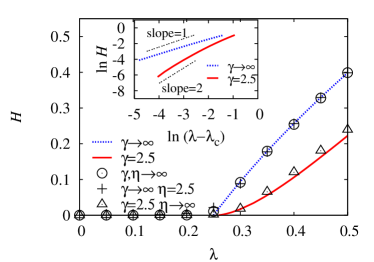
Figure 1: (Color online) Hamming distance $H$ for the Kauffman model as a function of $\lambda$. The points are the simulation results for model networks lee04npb with $N=10^{4}$ and $\langle k\rangle=4$ that have $P_{d}(k,q)=g_{\gamma}(k)g_{\eta}(q)$, where $g_{a}(x)\sim x^{-a}$ for $a$ finite and $g_{\infty}(x)=\langle k\rangle^{x}e^{-\langle k\rangle}/x!$. The Hamming distance $H$ was first averaged over time between $t=100$ and $t=200$, and then averaged over $1000$ different realizations of networks and regulating rules for which $H\neq 0$. The lines are the numerical solutions to Eq. (3) with $H(t)=\bar{H}(t)=H$ for all $t$ and the same degree distributions as in the simulation used. (Inset) Plots of $\ln H$ versus $\ln(\lambda-\lambda_{c})$ with $\lambda_{c}=0.25$. The slopes agree with Eq. (8).

The quantity $K$ may be considered as the average in-degree of regulators weighted by their out-degrees. Introducing the conditional average of out-degree, $q_{k}\equiv\sum_{q}qP_{d}(k,q)/P_{d}(k)$, we can rewrite the quantity $K$ as $K=\sum_{k}k(q_{k}/\langle q\rangle)P_{d}(k)$ and also the first relation in Eq. (3) as

$$\bar{H}(t+1)=\lambda\sum_{k}\frac{q_{k}}{\langle q\rangle}P_{d}(k)[1-(1-\bar{H}(t))^{k}].$$ (5)

If $q_{k}$ is independent of $k$ or (more strongly) the in-degree and the out-degree of a node is not correlated statistically, it follows that $q_{k}=\langle q\rangle$ for all $k$, $K$ reduces to the conventional average in-degree $\langle k\rangle\equiv\sum_{k}kP_{d}(k)$, and $H(t)=\bar{H}(t)$. The analyses of the transcriptional regulatory networks of E. coli and yeast show no significant variation of $q_{k}$ with $k$ lee08 and so we will assume in the following that $q_{k}=\langle q\rangle$ for all $k$. In Sec. IV.3, we will discuss how our results for the critical phenomena would be changed by the $k$-dependence of $q_{k}$. Under this assumption ($q_{k}=\langle q\rangle$), the Hamming distance $H(t)$ depends only on the in-degree distribution $P_{d}(k)$ and the dynamics parameter $\lambda$.

It has been shown that the scaling behavior of the average number of attractors with the system size remains to be the same for different out-degree distributions such as uniform, exponential, and power-law one oosawa02 . Our analysis based on the annealed approximation suggests further the irrelevance of the out-degree distribution to the Hamming distance. To confirm this as well as check the validity of the annealed approximation or Eq. (3), we performed simulations of the Kauffman model defined in Sec. II on an ensemble of model networks constructed as follows lee04npb : i) Each of $N$ nodes has two indices $i_{\rm in}$ and $i_{\rm out}$, which run from $1$ to $N$ respectively. The two indices are given independently to each node. ii) Choose a node $A$ with index $i_{\rm out}$ with probability $i_{\rm out}^{-\alpha_{\rm out}}/\sum_{j}j^{\alpha_{\rm out}}$. iii) Choose a node $B$ indexed $i_{\rm in}$ with probability $i_{\rm in}^{-\alpha_{\rm in}}/\sum_{j}j^{\alpha_{\rm in}}$. iv) Assign a link from the node $A$ to $B$ unless they are connected. v) Repeat ii) and iii) until the total number of links is $L$. The generated networks have $N$ nodes, $L$ links, and degree distribution given by $P_{d}(k,q)=P_{d}(k)P_{d}(q)$, where in-degree distribution takes the form $P_{d}(k)\sim k^{-\gamma}$ and the out-degree distribution takes the form $P_{d}(q)\sim q^{-\eta}$ with $\gamma=1+1/\alpha_{\rm in}$ and $\eta=1+1/\alpha_{\rm out}$. It is then obvious that $q_{k}=\langle q\rangle$ for all $k$. When $\alpha_{\rm in}=0$ and thus all the nodes can have an incoming link with equal probability, the in-degree distribution becomes a Poisson one, $P_{d}(k)=\langle k\rangle^{k}e^{-\langle k\rangle}/k!$. Thus the degree distribution may take power-law or Poissonian form depending on the values of $\alpha_{\rm in}$ and $\alpha_{\rm out}$ corresponding to scale-free (SF) networks or completely random networks, respectively. The simulation results (data points) shown in Fig. 1 are compared with the numerical solutions (lines) to Eq. (3), the annealed approximation, which show a good agreement and support the validity of the annealed approximation. Also it is shown that the Hamming distance is the same for different out-degree distributions.

The implication of Eq. (3) for SF networks has been discussed in Ref. aldana03 , where $P_{d}(k)=k^{-\gamma}/\zeta(\gamma)$ for $k=1,2,\ldots$ with $\zeta(x)$ the Rieman-zeta function. Based on the result that $\langle k\rangle=\zeta(\gamma-1)/\zeta(\gamma)<2$ for $\gamma>2.47875\ldots$, it was claimed aldana03 that the abundance of SF networks with $2<\gamma<2.5$ in nature and society can be attributed to the presence of both phases, stable and unstable, only in such networks. However, the values of $\langle k\rangle$ and $\gamma$ do not show such strong correlation in real networks. For instance, the average degree $\langle k\rangle$ ranges from $2.57$ (Internet router network) to $28.78$ (movie actor network) although the degree exponent $\gamma$ lies between $2$ and $3$ albert02 , which is possible due to the power-law behavior observed only asymptotically. We will show in the next section that root for the dynamical advantage of SF network lies elsewhere.

III.3 Critical exponents

Here we address the behavior of the Hamming distance around $\lambda_{c}$ for infinite system size. In that regime of $\lambda$, the Hamming distance is very small and its increase with $\lambda-\lambda_{c}$ can be characterized by a scaling exponent. This critical behavior of the Hamming distance is of interest to us because it shows how the network topology is related to the system’s dynamic response.

When the moments $\langle k^{n}\rangle=\sum_{k}P_{d}(k)k^{n}$ for all $n>0$ are finite, Eq. (3) can be written as

$$H\simeq\lambda\sum_{n=1}^{\infty}\frac{(-1)^{n+1}}{n!}\langle k^{n}\rangle H^{n}.$$ (6)

Keeping the leading terms, we find that $H\simeq(\lambda/\lambda_{c})H-\lambda\langle k^{2}\rangle H^{2}/2$, which gives

$$H\sim\Delta$$

with $\Delta\equiv\lambda/\lambda_{c}-1$ for $0<\Delta\ll 1$. This result can be represented as $H\sim\Delta^{\beta}$ with $\beta=1$, where we introduced the critical exponent $\beta$.

On the other hand, if $P_{d}(k)\simeq ck^{-\gamma}$ for $k\gg 1$ with $c$ a constant, $\langle k^{n}\rangle$ diverges as $ck_{\rm max}^{n+1-\gamma}/(n+1-\gamma)$ for $n\geq\lceil\gamma\rceil-1$ with $k_{\rm max}$ the largest in-degree and $\lceil x\rceil$ denoting the smallest integer not smaller than $x$. Applying the relation $\sum_{k>k_{\rm max}}P_{d}(k)\sim 1/N$ from the extreme value statistics gumbel58 , one can see that $k_{\rm max}$ scales as $N^{1/(\gamma-1)}$. The diverging terms in Eq. (6) have alternative signs and lead to non-analytic terms in $H$ as described below robinson51pr . For small $H$, Eq. (3) reads as $H\simeq\lambda\sum_{k}P_{d}(k)[1-e^{-kH}]$ and recalling the power-law form of $P_{d}(k)$, $P_{d}(k)\simeq ck^{-\gamma}$, we can utilize the fact that the Mellin transform of a function $F(\gamma,H)\equiv\sum_{k=1}^{\infty}k^{-\gamma}e^{-kH}$ is given by $\mathcal{F}(\gamma,s)=\int_{0}^{\infty}F(\gamma,H)H^{s-1}dH=\Gamma(s)\zeta(s+\gamma)$ with $\Gamma(x)$ the Gamma function robinson51pr . The inverse transform of $\mathcal{F}(\gamma,s)$ then is represented in terms of the poles of the Rieman-zeta function and the Gamma function, which gives $F(\gamma,H)=\int_{c-i\infty}^{c+i\infty}\mathcal{F}(\gamma,s)H^{-s}ds=\Gamma(1-\gamma)H^{\gamma-1}+\sum_{n=0}^{\infty}(-1)^{n}/n!\zeta(\gamma-n)H^{n}$ robinson51pr . Therefore we find that, for $P_{d}(k)\simeq ck^{-\gamma}$ logarithmic ,

$$H\simeq\lambda\sum_{n=1}^{\lceil\gamma\rceil-2}\frac{(-1)^{n+1}}{n!}\langle k^{n}\rangle H^{n}-\lambda c\Gamma(1-\gamma)H^{\gamma-1}+\mathcal{O}(H^{\lceil\gamma\rceil-1}).$$ (7)

If $\gamma>3$, the $H^{2}$ term is the next leading term in the right-hand-side of Eq. (7) and then the critical behavior is given by $H\sim\Delta$ as in the case of all $\langle k^{n}\rangle$ finite. On the other hand, if $2<\gamma<3$, the $H^{\gamma-1}$ term becomes the next leading term and we find that $H\simeq(\lambda/\lambda_{c})H-\lambda c\Gamma(1-\gamma)H^{\gamma-1}$. Therefore for $\lambda>\lambda_{c}$,

$$H\sim\Delta^{1/(\gamma-2)}.$$

In summary, we can list the values of the critical exponent $\beta$ varying with the in-degree exponent $\gamma$ as lee07

$$\beta=\left\{\begin{array}[]{ll}1&(\gamma>3),\\ 1/(\gamma-2)&(2<\gamma<3),\end{array}\right.$$ (8)

which is confirmed numerically [See the inset of Fig. 1].

Figure 2: (Color online) Phase diagram of the Kauffman model for (a) a Poisson in-degree distribution and (b) a power-law one with the exponent $\gamma=2.5$, both in case of uncorrelated in- and out-degree. The color encodes the Hamming distance $H$ obtained by numerically solving Eq. (3) under setting $H(t)=\bar{H}(t)=H$.

Figure 3: Finite-size scaling behavior in the critical regime. (a) Data collapse for different system sizes with $\gamma\to\infty$. The inset shows that $\lambda_{c}\simeq 0.2505(5)$. (b) Data collapse with $\gamma=2.5$ and $\lambda_{c}\simeq 0.287(1)$.

The critical exponent $\beta$ varying with the in-degree distribution as in Eq. (8) is illuminating how the network topology affects the system’s response to perturbation. Figure 2 shows phase diagrams of the Kauffman model on model networks with a Poisson in-degree distribution and with a power-law in-degree distribution with the exponent $\gamma=2.5$, in which color represents the value of the Hamming distance. As shown in the figure, the SF networks with $2<\gamma<3$ and thus larger values of $\beta$ keep the Hamming distance non-zero but small in a much larger region in the $(\lambda,\langle k\rangle)$ plane than those with $\gamma>3$. Structural and functional organization of cellular networks, parameterized here by $\langle k\rangle$ and $\lambda$ ($p$), respectively, may be subject to unexpected changes. Our finding suggests that the systems with strong heterogeneous connectivity patterns can maintain their dynamic criticality robustly, and further, votes for the hypothesis that living organism’s machinery lies at the edge of chaos.

IV Boolean networks of finite size

In the thermodynamic limit $N\to\infty$, the critical point does not exhibit any dependence on the network topology. However, for finite $N$, the critical point itself develops its dependence on the network topology: It is no more a point but has a non-zero width depending on $N$. Adopting the finite-size scaling ansatz marroBook99

$$H=N^{-\beta/\mu}\ \Psi(\Delta N^{1/\mu})$$ (9)

with the scaling function $\Psi(x)\to$ const. for $x\ll 1$ and $\Psi(x)\to x^{\beta}$ for $x\gg 1$, one can see that $H\sim N^{-\beta/\mu}$ in the critical regime $|\Delta N^{1/\mu}|\ll 1$. In the $\lambda$ axis, this critical regime is $N^{-1/\mu}$ wide for $N$ finite and shrinks to zero in the thermodynamic limit. Therefore the scaling exponent $\mu$ describes the width of the critical regime for finite-size systems. In the critical regime, the cluster of perturbed nodes, explained below, exhibits scale invariance characterized by a power-law distribution of its size, which is connected to the behavior $H\sim N^{-\beta/\mu}$. We show in the next that the asymptotic behavior of the cluster size distribution can be derived using Eqs. (6) and (7), which allows us to obtain the scaling exponent $\mu$ and to check Eq. (9).

IV.1 Evolution of perturbed-node clusters

The parameter $\lambda$ denotes the probability that a node becomes perturbed ($\sigma_{i}(t+1)\neq\hat{\sigma_{i}}$) once the configuration of its neighbors are perturbed ($\Sigma_{i}\neq\hat{\Sigma_{i}}$). When $\lambda$ is zero, the Hamming distance becomes zero immediately even though all nodes were perturbed initially. As $\lambda$ increases from $0$, clusters appear, consisting of perturbed nodes that are connected by active edges. An edge from node $A$ to $B$ is inactive if the perturbation at node $A$ cannot bring any difference to the dynamical state of node $B$, and active otherwise. While a node’s state can be totally irrelevant to its neighbor connected by an inactive edge, perturbation at one node can propagate to its neighbors through active edges. The perturbed-node clusters evolve with time, decaying or growing. A perturbed node may become normal (non-perturbed) due to its regulators becoming normal at a certain time step, which leads to the decay of the cluster it belonged to. On the other hand, normal nodes may become perturbed due to its regulators becoming perturbed, which leads to the growth of a cluster.

When the parameter $\lambda$ reaches the critical regime or goes beyond it ($\lambda\gtrsim\lambda_{c}$), a giant cluster of perturbed nodes appears and contributes to the Hamming distance in the stationary state. There may exist many smaller clusters, but they are hard to survive eventually. A small cluster has a relatively small number of perturbed nodes, and they are surrounded by many normal nodes. Therefore the perturbed nodes in smaller clusters have higher chance of becoming normal than those in larger clusters, which leads to the higher chance of shrinking and decaying of smaller clusters. The perturbed nodes in the giant cluster, on the other hand, have more perturbed nodes as regulators and thus the giant cluster has a higher chance to survive; the probability becomes nonzero when $\lambda\gtrsim\lambda_{c}$. Therefore the Hamming distance $H$ can be approximated using the size of the largest cluster $S$ via $H\sim S/N$ aharony . We will use this relation in the below to derive the asymptotic behavior of the size distribution of the clusters from the self-consistent equations for $H$, Eqs. (6) and (7).

IV.2 Cluster-size distribution in the annealed approximation

Let us denote the probability that a node belongs to a size-$s$ cluster (of perturbed nodes) by $P(s)$ and consider its generating function $\omega=\mathcal{P}(z)=\sum_{s}P(s)z^{s}$. The Hamming distance is related to the generating function as

$$H\simeq{S\over N}\simeq 1-\sum_{s<S}P(s)\simeq\lim_{N\to\infty}[1-\mathcal{P}(z_{N}^{*})],$$ (10)

where $z_{N}^{*}=e^{-1/\tilde{S}}$ and $\tilde{S}$ satisfies $S_{2}\ll\tilde{S}\ll S$ with $S_{2}$ the second largest cluster size. This relationship, combined with Eqs. (6) and (7), gives us the functional form of the inverse function $z=\mathcal{P}^{-1}(\omega)$. Let’s expand the inverse function around $\omega=1$ as $z=1-\sum_{n\geq 1}b_{n}(1-\omega)^{n}$. Then one can see that this equation should reduce to Eqs. (6) or (7), depending on the in-degree distribution, with $z$ and $1-\omega$ replaced by $z_{N}^{*}$ and $H$, respectively, in the thermodynamic limit. Note that $z_{N}^{*}\to 1$ in the thermodynamic limit. Therefore the inverse function $z=\mathcal{P}^{-1}(\omega)$ is expanded around $\omega=1$ as follows:

$$1-z\simeq(1-\lambda/\lambda_{c})(1-\omega)+\lambda\langle k^{2}\rangle(1-\omega)^{2}/2+\cdots$$ (11)

for $\gamma>3$ and

$$1-z\simeq(1-\lambda/\lambda_{c})(1-\omega)+\lambda c\Gamma(1-\gamma)(1-\omega)^{\gamma-1}+\cdots$$ (12)

for $2<\gamma<3$, where $c$ is the coefficient appearing in the asymptotic behavior of the in-degree distribution $P_{d}(k)\simeq ck^{-\gamma}$.

The functional behavior of $\mathcal{P}(z)$ around $z=1$ is then derived from Eqs. (11) and (12). At the critical point ($\lambda=\lambda_{c}$), it exhibits a singularity depending on the in-degree exponent:

$$1-\mathcal{P}(z)\sim\left\{\begin{array}[]{ll}(1-z)^{1/2}&(\gamma>3)\\ (1-z)^{1/(\gamma-1)}&(2<\gamma<3)\end{array}\right.$$ (13)

The asymptotic behavior of the cluster-size distribution $P(s)$ can be obtained from the functional form of $\mathcal{P}(z)$ since $P(s)=(1/s!)(d^{s}/dz^{s})\mathcal{P}(z)|_{z=0}$. In particular, when $1-\mathcal{P}(z)\sim(1-z)^{\tau-1}$ with $\tau$ a non-integer, the cluster-size distribution takes a power-law form $P(s)\sim s^{-\tau}$. The asymptotic behavior of $P(s)$ is thus distinguished between $\gamma>3$ and $2<\gamma<3$ as follows:

$$P(s)\sim\left\{\begin{array}[]{ll}s^{-3/2}&(\gamma>3),\\ s^{-\gamma/(\gamma-1)}&(2<\gamma<3).\end{array}\right.$$ (14)

Scale invariance is typical of the system at the critical point and the power-law form of the cluster-size distribution is an example aharony . Our finding shows that the power-law exponent may vary with the degree exponent. In the subcritical ($\lambda<\lambda_{c}$) or supercritical ($\lambda>\lambda_{c}$) regime, the linear term in $1-\omega$ in Eqs. (11) and (12) is dominant around $\omega=1$ and the cluster-size distribution takes an exponential-decaying form like $P(s)\sim e^{-s/s_{c}}$ lee04npb .

IV.3 Scaling exponents

Once the asymptotic behavior of $P(s)$ is known, the scaling property of the largest cluster size may be derived. Using Eq. (14) in the relation $\sum_{s>S}P(s)\sim S/N$, a part of Eq. (10), one can see that the size of the largest cluster $S$ scales with the system size $N$ as $S\sim N^{2/3}$ for $\gamma>3$ and $S\sim N^{(\gamma-1)/\gamma}$ for $2<\gamma<3$. It is known that the number of nonfrozen nodes in critical Boolean networks with any fixed number of inputs kaufman05 ; mihaljev06 or fast-decaying in-degree distribution also scales as $N^{2/3}$ samuelsson06 . A node $i$ is called nonfrozen if its state ($\sigma_{i}$) is not fixed at either $0$ or $1$ in the stationary state and thus may be perturbed (but not necessarily). The set of perturbed nodes is thus a subset of the set of nonfrozen nodes and it is noteworthy that their sizes display the same scaling behavior.

The Hamming distance, $H\sim S/N$, in the critical regime is then given by

$$H\sim\left\{\begin{array}[]{ll}N^{-1/3}&(\gamma>3),\\ N^{-1/\gamma}&(2<\gamma<3).\end{array}\right.$$ (15)

Since $H\sim N^{-\beta/\mu}$ in the critical regime from the finite-size scaling ansatz in Eq. (9), we find that the scaling exponent $\mu$ is given by

$$\mu=\left\{\begin{array}[]{ll}3&(\gamma>3),\\ \gamma/(\gamma-2)&(2<\gamma<3).\end{array}\right.$$ (16)

To check numerically the derived finite-size scaling behavior of the Hamming distance, we performed simulations of the Kauffman model on the model networks described in Sec. III.2 varying the system size. First, we plot the data of $HN^{\beta/\mu}$ as a function of $\lambda$ for the same average degree ($\langle k\rangle=4$) and different system sizes ($N=4000,8000,16000,32000$). They cross at one point, which determines the critical point $\lambda_{c}$ according to Eq. (9) (See the insets of Fig. 3). Using these values of $\lambda_{c}$, we plotted the same data of $HN^{\beta/\mu}$ versus $\Delta N^{1/\mu}$ in Fig. 3. The collapse of the data from different system sizes, while a slight deviation is seen in case of SF networks, presumably due to strong finite-size effects, supports the scaling behavior of the Hamming distance in Eq. (9) with Eqs. (8) and (16) used.

The finite-size scaling behavior in Eq. (9) has been identified also in a wide range of dynamical systems on complex networks. In particular, the formation of a giant cluster in SF networks evolving by adding links has been analyzed through its exact mapping to the $q=1$ Potts model and found to be characterized by $(\beta=1,\ \mu=3)$ for the degree exponent $\gamma>4$ and $(\beta=1/(\gamma-3),\ \mu=(\gamma-1)/(\gamma-3))$ for $3<\gamma<4$ lee04npb . These exponents are very similar to Eqs. (8) and (16). Also in the Ising model aleksiejuk02 ; leone02 ; igloi02 ; herrero04 and the Kuramoto model for synchronization phenomena hong02 ; lee05 , the exponents are given by $(\beta=1/2,\ \mu=2)$ for the degree exponent $\gamma>5$ and $(\beta=1/(\gamma-3),\ \mu=(\gamma-1)/(\gamma-3))$ for $3<\gamma<5$. Such similar dependence of the scaling exponents on the degree exponent suggests a common framework to understand the critical phenomena on complex networks igloi02 ; dorogovtsev02 ; hong07 .

We note that while the scaling plot gives $\lambda_{c}\simeq 0.251$ for the completely random networks ($\gamma\to\infty$) as predicted by Eq. (4), the SF networks with $\gamma=2.5$ have $\lambda_{c}\simeq 0.289$, deviating from the predicted value $0.25$. This deviation seems to be rooted in the use of the annealed approximation for the Hamming distance. It has been reported that the analytic prediction of the critical point in the framework of the mean-field theory deviates slightly from the numerical analysis in the Ising model herrero04 and in the Kuramoto model for synchronization phenomena lee05 . An improvement can be made by considering the Cayley tree with a given degree distribution as the underlying network topology dorogovtsev02 .

Our results show that the width of the critical regime $W\sim N^{-1/\mu}$ in the $\lambda$ axis increases as the in-degree exponent $\gamma$ decreases below $3$ while its scaling behavior remains the same for all $\gamma>3$. Since the number of genes in most organisms is not infinite but of order $10^{5}$ at most, the width of the critical regime may be between $\mathcal{O}(10^{-2})$ and $\mathcal{O}(1)$, depending on the in-degree exponent. Such a broad critical regime for small values of $\gamma$ should help living organisms to remain in the critical regime and in turn, to balance between robustness and evolvability. Individual dynamical responses depend on the properties of the perturbed elements, i.e,, on their connectivities and regulating rules, which leads to perturbation propagation on various scales in heterogeneous networks aldana03 . Here we have analyzed the whole ensemble of such differentiated dynamical responses in heterogeneous networks and found that it can remain critical more easily with the help of extremely heterogeneous connectivity patterns.

The effects of correlation between in- and out-degree of the same node, which we have ignored so far, can be addressed in the results we obtained. In presence of the in- and out-degree correlation, $(q_{k}/\langle q\rangle)P_{d}(k)$ should be considered instead of $P_{d}(k)$ to compute the Hamming distance, as seen in Eq. (5). If it holds that $q_{k}\sim k^{-\theta}$ for large $k$, we have to consider the effective in-degree exponent, $\gamma_{\rm eff}=\gamma+\theta$, in place of $\gamma$ for power-law in-degree distributions in all the results we obtained, including the scaling exponents in Eqs. (8) and (16).

V Summary and Discussion

In summary, we investigated the phase transition between the stable (ordered) and unstable (chaotic) phase in the Boolean dynamical network. Heterogeneous connectivities are found to broaden substantially the small Hamming distance region close to the phase boundary by suppressing the perturbation propagation in the unstable phase. Furthermore the transition region for finite system sizes turns out to be much wider than in homogeneous networks. Such a robust pseudo-criticality is expected to be also present in transcriptional regulatory networks and also in other biological networks such as neural networks bornholdt03 , which can be a source for stability and evolvability coexisting in living organisms.

Our results suggest that the heterogeneous connectivity patterns of many biological networks have been selected in the course of evolution in part to serve for achieving stability and evolvability simultaneously. Therefore it would be desirable to propose a model in which heterogeneous connectivity patterns emerge driven by the evolutionary pressure towards a broad edge of chaos. There are indeed models for co-evolution of network structure and dynamics, which reproduce networks with a selected number of links supporting dynamic criticality by dynamics-correlated addition and deletion of links bornholdt00 ; liu06 . Similarly to these models, if one allows link rewiring only, preserving the total number of links, and make it happen depending on the network’s dynamical state, the network is expected to be organized so as to have a broad degree distribution, which is under investigation.

While we focussed on the Hamming distance to capture the effects of structural features on the dynamic stability of Boolean networks, it would be also interesting to see how the heterogeneous connectivity patterns affect the properties of attractors in the configuration space, given the recent interests bastolla98 ; bilke01 ; samuelsson03 ; drossel05 ; klemm05 in the scaling behavior of the number and length of the attractors in the critical Boolean networks. It has been shown that the median attractor length of SF networks is larger than that of networks with fixed in-degree at the critical point iguchi07 ; kinoshita07 , but much more properties remain to be investigated.

The asymptotic behaviors of the in-degree distributions of real transcriptional regulatory networks of E. coli shenorr02 and yeast tilee02 ; luscombe04 are hard to discern due to finite size effects. In both organisms, there are about one hundred regulators (nodes with outgoing links), which impose a cut-off in the measured in-degree distributions. However, one can find for the network of yeast that its in-degree distribution is much broader than that of the networks generated by randomly rewiring the links, and that the Hamming distance of the Boolean dynamics is much slower than that in the randomized networks, demonstrating the contribution of heterogeneous connectivity pattern to maintaining dynamic criticality lee07 .

It should be noted that the real transcriptional regulatory networks and other biological networks have much richer structural properties than described here and their relation to the dynamic criticality of the system is of interest. For example, the correlation of the degrees of neighboring nodes has been identified in many real-world networks pastorsatorras01 ; newman02 including the yeast gene regulatory network balcan05 and there are studies on the effects of the degree-degree correlation on the structure and dynamics of complex networks vazquez03 ; bianconi06 ; noh07 . While it has been shown noh07 that a negative (positive) degree-degree correlation is irrelevant (relevant) to the percolation transition in complex networks, it still remains to be addressed how the correlation affects the critical phenomena of Boolean networks.

References

- (1)
- (2) D. Thieffry, A. M. Huerta, E. Pérez-Rueda, and J. Collado-Vides, Bioessays 20, 433 (1998).
- (3) T. I. Lee et al., Science 298, 799 (2002).
- (4) R. Dobrin, Q. K. Beg, A.-L. Barabási, and Z. N. Oltvai, BMC Bioinformatics 5, 10 (2004).
- (5) N. Guelzim, S. Bottani, P. Bourgine, and F. Képès, Nature Genetics 31, 60 (2002).
- (6) S. S. Shen-Orr, R. Milo, S. Mangan, and U. Alon, Nature Genetics 31, 64 (2002).
- (7) M. M. Babu et al., Curr. Opin. Struct. Biol 14, 283 (2004).
- (8) S. Kauffman, J. Theor. Biol 22, 437 (1969); The Origins of Order: Self-organization and Selection in Evolution (Oxford Univ. Press, Oxford, 1993).
- (9) B. Derrida and Y. Pomeau, Europhys. Lett. 1, 45 (1986).
- (10) M. Aldana, S. Coppersmith, and L.P. Kadanoff, in Perspectives and Problems in Nonlinear Science. A celebratory volule in honor of Lawrence Sirovich. Springer Applied Mathematical Sciences Series. E. Kaplan, J.E. Marsden, and K.R. Sreenivasan Eds. (2003).
- (11) U. Bastolla and G. Parisi, Physica D 115, 203 (1998); 219 (1998).
- (12) S. Bilke and F. Sjunnesson, Phys. Rev. E 65, 016129 (2001).
- (13) B. Samuelsson and C. Troein, Phys. Rev. Lett. 90, 098701 (2003).
- (14) B. Drossel, T. Mihaljev, and F. Greil, Phys. Rev. Lett. 94, 088701 (2005).
- (15) K. Klemm and S. Bornholdt, Phys. Rev. E 72, 055101(R) (2005).
- (16) S. E. Harris, B. K. Sawhill, A. Wuensche, and S. Kauffman, Complexity 7, 23 (2002).
- (17) S. Kauffman, C. Peterson, B. Samuelsson, and C. Troein, Proc. Natl. Acad. Sci. U.S.A. 100, 14796 (2003).
- (18) R. Albert and A.-L. Barabási, Rev. Mod. Phys. 74, 47 (2002)
- (19) D.-S. Lee and H. Rieger, J. Theor. Biol. 248, 618 (2007).
- (20) S. Kauffman, C. Peterson, B. Samuelsson, and C. Troein, Proc. Natl. Acad. Sci. U.S.A. 101, 17102 (2004).
- (21) D. Balcan, A. Kabakçioğlu, M. Mungan, and A. Erzan, PLoS One 2, e501 (2005).
- (22) N.M. Luscombe, M.M. Babu, H. Yu, M. Snyder, S.A. Teichmann, and M. Gerstein, Nature 431, 308 (2004).
- (23) A. A. Moreira and L. A. N. Amaral, Phys. Rev. Lett. 94, 218702 (2005).
- (24) C. Oosawa and M. A. Savageau, Phyisca D 170, 143 (2002).
- (25) M. Aldana and P. Cluzel, Proc. Natl. Acad. Sci. U.S.A. 100, 8710 (2003).
- (26) D.-S. Lee, unpublished data (2008).
- (27) D.-S. Lee, K.-I. Goh, B. Kahng, and D. Kim, Nucl. Phys. B 696, 351 (2004).
- (28) E.J. Gumbel Statistics of Extremes (Columbia Univ. Press, New York, 1958).
- (29) J.E. Robinson, Phys. Rev. 83, 678 (1951).
- (30) There is a logarithmic term in Eq. (7) in case of an integer robinson51pr .
- (31) J. Marro and R. Dickman, Nonequilibrium Phase Transitions in Lattice Models (Cambridge Univ. Press, Cambridge, 1999).
- (32) D. Stauffer and A. Aharony, Introduction to percolation theory (Taylor & Francis, London, 1994).
- (33) V. Kaufman, T. Mihaljev, and B. Drossel, Phys. Rev. E 72, 046124 (2005).
- (34) T. Mihaljev, and B. Drossel, Phys. Rev. E 74, 046101 (2006).
- (35) B. Samuelsson, and J.E. Socolar, Phys. Rev. E 74, 036113 (2006).
- (36) A. Aleksiejuk, J.A. Holyst, and D. Stauffer, Physica A 310, 260 (2002).
- (37) M. Leone, A. Vázquez, A. Vespignanai, and R. Zecchina, Eur.Phys.J.B 28, 191 (2002).
- (38) F. Iglói, and L. Turban, Phys. Rev. E 66, 036140 (2002).
- (39) C.P. Herrero, Phys. Rev. E 69, 067109 (2004).
- (40) H. Hong, M.Y. Choi, and B.J. Kim, Phys. Rev. E 65, 026139 (2002).
- (41) D.-S. Lee, Phys. Rev. E 72, 026208 (2005).
- (42) S.N. Dorogovtsev, A.V. Goltsev, and J.F.F. Mendes, Phys. Rev. E 66, 016104 (2002).
- (43) H. Hong, M. Ha, and H.Park, Phys. Rev. Lett. 98, 258701 (2007).
- (44) S. Bornholdt and T. Röhl, Phys. Rev. E 67, 066118 (2003).
- (45) S. Bornholdt and T. Rohlf, Phys. Rev. Lett. 84, 6114 (2000).
- (46) M. Liu and K.E. Bassler, Phys. Rev. E 74, 041910 (2006).
- (47) K. Iguchi, S. Kinoshita, and H.S. Yamamda, J. Theor. Biol. 247, 138 (2007).
- (48) S. Kinoshita, K. Iguchi, and H.S. Yamamda, AIP Conference Proceedings 982, 2128 (2008).
- (49) R. Pastor-Satorras, A. Vazquez, and A. Vespignani, Phys. Rev. Lett. 87, 258701 (2001).
- (50) M.E.J. Newman, Phys. Rev. Lett. 89, 208701 (2002).
- (51) A. Vazquez and Y. Moreno, Phys. Rev. E 67, 015101(R) (2003).
- (52) G. Bianconi and M. Marsili, Phys. Rev. E 76, 026116 (2007).
- (53) J.D. Noh, Phys. Rev. E 76, 026116 (2007).