Stable particles in anisotropic spin-1 chains

Abstract

Motivated by field-theoretic predictions we investigate the stable excitations that exist in two characteristic gapped phases of a spin-1 model with Ising-like and single-ion anisotropies. The sine-Gordon theory indicates a region close to the phase boundary where a stable breather exists besides the stable particles, that form the Haldane triplet at the Heisenberg isotropic point. The numerical data, obtained by means of the Density Matrix Renormalization Group, confirm this picture in the so-called large-$D$ phase for which we give also a quantitative analysis of the bound states using standard perturbation theory. However, the situation turns out to be considerably more intricate in the Haldane phase where, to the best of our data, we do not observe stable breathers contrarily to what could be expected from the sine-Gordon model, but rather only the three modes predicted by a novel anisotropic extension of the Non-Linear Sigma Model studied here by means of a saddle-point approximation.

1 Introduction

One-dimensional spin systems have been largely studied since Haldane haldane83 proposed his conjecture. He suggested that while half-odd integer spin chains should always be gapless, integer-spin ones should manifest a gap. The conjecture is supported by a field-theoretic analysis aue of the lattice Hamiltonians, a typical approach for low-dimensional quantum systems that admit a continuum-limit counterpart in $(D+1)$ dimensions. The low-energy spectrum of the spin Hamiltonian can be interpreted in the language of (quasi)particles: a finite energy gap corresponds to a massive particle at rest, and the dispersion relation of the excitation for small momenta can be read as a relativistic (on shell) energy-momentum relation. The field-theoretic approach proved to be extremely powerful to explain experimental data. For instance, recent observations on spin-1/2 compounds with Dzyaloshinskii-Moriya interaction in external field asano2000 ; kenzelmann2004 ; zyagin2004 , confirm the appearence of effective particles, namely solitons and breathers, as predicted by the Sine-Gordon Model (SGM) that describes the low energy spectrum of the chain.

In this paper we discuss the possibility of observing solitons and possibly breathers in spin-1 chains with internal anisotropies. In particular, it is important to understand the role of the interactions between the particles of the continuum theory to see how their bound and scattering states manifest in the energy spectrum of the lattice model. The effective interactions will depend on the values of parameters of the spin Hamiltonian and it is possible that certain two- (or more) particle states that are stable in a region of parameter space loose their stability when the parameters are continuously changed. In other terms the formerly stable state acquires a rest mass equal or larger than the sum of the rest masses of its constituents and, if there are no special selection rules, the particle decays into the continuum part of the spectrum.

In this paper we study such a scenario for the following spin-1 anisotropic model:

$$H=\sum_{j=1}^{L}\left\{S_{j}^{x}S_{j+1}^{x}+S_{j}^{y}S_{j+1}^{y}+\lambda S_{j}^{z}S_{j+1}^{z}+D\left(S_{j}^{z}\right)^{2}\right\},$$ (1)

where $\lambda$ and $D$ parametrize the Ising-like and single-ion anisotropies respectively. This Hamiltonian is known to be described, in the continuum low-energy limit, by a Non-Linear Sigma Model (NL$\sigma$M) in the vicinity of the isotropic antiferromagnetic Heisenberg point ($\lambda=1,\,D=0$) haldane83 ; aue , and the SGM in the neighborhood of the critical line separating two gapped phases, namely the large-$D$ and the Haldane ones on_c1_line . These phases will be defined in section 2, where we will also recall the mapping onto the SGM and present a novel extension of the NL$\sigma$M for anisotropic integer-spin models which encompasses the usual isotropic NL$\sigma$M that lies at the basis of the Haldane conjecture. In general we find a triplet of excitations and no other bound states. On the contrary, from a quantitative analysis of the SGM we expect that in some region of the Haldane and large-$D$ phases at least an additional bound state (a breather) should appear. We proceed in section 3 to a numerical check of these expectations using the multi-target Density Matrix Renormalization Group (DMRG) technique that allows us to handle chains of up to 100 sites and extract various excited states of the spectrum. The data in the large-$D$ phase confirm the existence of a breather in the region predicted by the SGM. On the other hand, we do not find any stable breather in the Haldane phase. In section 4 we will sketch also a simple perturbative argument that provides a quantitative interpretation of the data. Finally, in section 5 we will comment on our results and draw some general conclusions.

2 Quantum field theories for the $\lambda-D$ model

Among integer spin models, the anisotropic $S=1$ chain with its rich phase diagram occupies a relevant position. At the isotropic point, ($\lambda=1$, $D=0$) the ${\rm O}(3)$ Heisenberg model is recovered. The full phase diagram consists of six different phases (see chs for a recent numerical determination). We will focus our attention on the $\lambda>0$ half-plane where, apart from the transition lines, all the phases show a nonzero energy gap above the ground state (GS). In fig. 1 we report the phase diagram in this range of parameters. Usually, two different types of order parameters are used to characterize these phases: the Néel order parameters (NOP):

$${\cal O}_{N}^{\alpha}=\lim_{|i-j|\rightarrow\infty}(-1)^{i-j}\langle S_{i}^{\alpha}S_{j}^{\alpha}\rangle;\;\alpha=x,y,z$$ (2)

and the string order parameters (SOP):

$${\cal O}_{S}^{\alpha}=-\lim_{|i-j|\rightarrow\infty}\langle S_{i}^{\alpha}{\rm e}^{{\rm i}\pi\sum_{k=i+1}^{j-1}S_{k}^{\alpha}}S_{j}^{\alpha}\rangle;\;\alpha=x,y,z\,,$$ (3)

first introduced by den Nijs and Rommelse nijs_rom . For $D\gg 1$ and $D\gtrsim\lambda$ the system is in the so-called large-$D$ phase, with a unique GS that does not break the above symmetry: $\mathcal{O}_{S}^{\alpha}=\mathcal{O}_{N}^{\alpha}=0$ for all $\alpha$. Decreasing $D$, for $\lambda\lesssim 3$, we have a transition into the Haldane phase. This phase is characterized by the non-vanishing of all the components of the SOP’s $\mathcal{O}_{S}^{\alpha}\neq 0$, meaning that the ${\rm Z}_{2}\times{\rm Z}_{2}$ symmetry is fully broken, and by $\mathcal{O}_{N}^{\alpha}=0\,\,\forall\alpha$. Inside the Haldane phase, the gap of the first excited state, though always different from zero, belongs to two different spin sectors depending on the parameters $\lambda$ and $D$. It belongs to the $S_{{\rm tot}}^{z}=\pm 1$ sector for values of $\lambda$ and $D$ above the so-called degeneracy line (see fig. 1). This line, which passes through the ${\rm O}(3)$ isotropic point, divides the Haldane phase into two sub-phases botet . Below this line the first excited state has $S_{{\rm tot}}^{z}=0$. The GS is always unique and belongs to the $S_{{\rm tot}}^{z}=0$ sector. On the right of the Haldane phase we find the twofold degenerate Néel phase. Here the ${\rm Z_{2}}\times{\rm Z}_{2}$ symmetry is only partly broken as as proved by the fact that $\mathcal{O}_{N}^{\alpha}=\mathcal{O}_{S}^{\alpha}=0$ for $\alpha=x,y$ but $\mathcal{O}_{N}^{z},\,\mathcal{O}_{S}^{z}\neq 0$. The Haldane-large-$D$ (H-D) and Haldane-Néel (H-N) transition lines mark second order transitions; the former is described by a $c=1$ Conformal Field Theory (CFT) while the latter by a $c=1/2$ CFT. They merge at the tricritical point ($\lambda\cong 2.90$, $D\cong 3.20$) on_c1_line where the Haldane phase disappears and the large-$D$-Néel transition becomes first order.

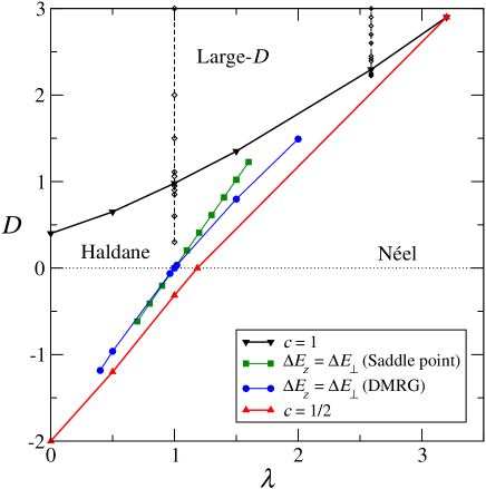
Figure 1: Phase diagram of the model (1) obtained numerically via DMRG. The two lines passing through the isotropic point are the loci of points where the transverse and longitudinal gaps coincide. Circles are DMRG data whereas squares are the results of the theoretical approach. The vertical lines across the Haldane-large-$D$ transitions join the points studied numerically (see section 3).

Near the isotropic point the Hamiltonian (1) can be mapped onto an anisotropic version of the NL$\sigma$M using Haldane’s ansatz aue to decompose the spin coherent states field $\vec{\Omega}_{j}(\tau)=\vec{n}_{j}(\tau)(-1)^{j}\sqrt{1-\frac{\ell_{j}^{2}(\tau)}{S^{2}}}+\frac{\vec{\ell_{j}}(\tau)}{S}$ into a uniform, $\vec{\ell_{j}}(\tau)$, and a staggered part $\vec{n}_{j}(\tau)=[\mathbf{n}_{j\perp}(\tau),n_{jz}(\tau)]$, satisfying the constraint $|\mathbf{n}_{\perp}|^{2}+n_{z}^{2}=1$. After integration of the uniform field, one obtains the following effective Lagrangian density:

$$\mathcal{L} = \frac{v_{\perp}}{2g_{\perp}}\left[|\partial_{x}{\bf\mathbf{n}}_{\perp}|^{2}+\frac{1}{v_{\perp}^{2}}|\partial_{\tau}\mathbf{n}_{\perp}|^{2}\right]+$$ (4)

$$\frac{v_{z}}{2g_{z}}\left[\left(\partial_{x}n_{z}\right)^{2}+\frac{1}{v_{z}^{2}}\left(\partial_{\tau}n_{z}\right)^{2}+\mu_{z}n_{z}^{2}\right]+\mathcal{L}_{\textrm{int}},$$

where the interaction term has a simple expression only in the regions $|n_{z}|\ll 1$ and $|\mathbf{n}_{\perp}|\ll 1$. In the first region the interaction term has the form

$$\mathcal{L}_{\textrm{int}}=n_{z}^{2}\left[d_{\perp}\left|\partial_{\tau}\mathbf{n}_{\perp}\right|^{2}+d_{z}(\partial_{\tau}n_{z})^{2}\right],$$

whereas, in the region $\left|{\bf\mathbf{n}}_{\perp}\right|\ll 1$, the interaction term has the form

$$\mathcal{L}_{\textrm{int}}=\left|\mathbf{n}_{\perp}\right|^{2}\left[d_{\perp}\left|\partial_{\tau}\mathbf{n}_{\perp}\right|^{2}+d_{z}(\partial_{\tau}n_{z})^{2}\right].$$

Here the constants $g_{\perp\left(z\right)},\,v_{\perp\left(z\right)},\,d_{\perp\left(z\right)},\,\mu_{z}$ are different functions of the microscopic parameters $\lambda$ and $D$ whose explicit expressions depend on the region one considers.

As long as one deals with integer spins the topological term arising from the combination of the Berry phases on each site reduces to a multiple of $2\pi$ and therefore can be safely omitted. More details on the mapping into this anisotropic variant of the NL$\sigma$M can be found in ref. pas .

The constraint of unit norm makes the theory hard to treat. In both regions, $\left|n_{z}\right|\ll 1$ and $\left|{\bf\mathbf{n}}_{\perp}\right|\ll 1$, we limit ourselves to a mean-field solution that can be worked out using the saddle-point approximation on eq. (4). The constraint is taken into account by introducing a uniform Lagrange multiplier $\eta$. We refer the reader to ref. pas for details and only mention that one arrives at a couple of self-consistent equations for the longitudinal and transverse gaps $\Delta E_{z}$ and $\Delta E_{{\rm\perp}}$, that play the role of the masses of the particles of an “anisotropic Haldane triplet”. Of course $\Delta E_{z}=\Delta E_{\perp}$ at the isotropic Heisenberg point. However, when $\lambda$ and $D$ are varied the transverse and longitudinal channels split. Nonetheless, guided by the numerical work of botet , we can search for a specific line in parameter space where the two gaps remain degenerate (in the thermodynamic limit) even if the lattice theory has no ${\rm O}(3)$ symmetry. Interestingly, the line found through the self-consistent equations is in good agreement with the one found with the DMRG as depicted in fig. 1.

Let us now see a possible connection with the SGM. Neglecting the longitudinal field (i.e. setting $n_{z}=0$) and writing $\mathbf{n}_{\perp}=\mathrm{e}^{i\theta}$, then an ${\rm O}(2)$ NL$\sigma$M is recovered:

$$\mathcal{L}=\frac{1}{2}v\left[\left(\partial_{x}\Theta\right)^{2}+\frac{1}{v^{2}}\left(\partial_{\tau}\Theta\right)^{2}\right]$$ (5)

with $\Theta=\theta/g$, $g=\sqrt{(2+2\lambda+D)}$ and $v=g$ (for $S=1$) . This is exactly a free Gaussian model with a bosonic field compactified along a circle of radius $1/\sqrt{g}$. We know that this model describes a CFT with central charge $c=1$ and with primary fields having scaling dimensions:

$$d_{mn}=\left(\frac{m^{2}}{4K}+n^{2}K\right),$$ (6)

with $K=\pi/g$ and $m,n\in\mathbb{Z}$.

In a previous work on_c1_line it was argued that near the Gaussian $c=1$ line the perturbed ${\rm O}(2)$ model can written in terms of a sine-Gordon model:

$${\cal L}=\frac{1}{2}\left[v\left(\partial_{x}\Phi\right)^{2}+\frac{1}{v}\left(\partial_{\tau}\Phi\right)^{2}\right]+\frac{v\bar{\mu}}{a^{2}}\cos(\sqrt{4\pi K}\Phi)$$ (7)

where $\Phi$ is a compactified field dual to $\Theta$, $a$ is the lattice spacing and $\bar{\mu}$ is a coupling constant that should vanish exactly along the H-D transition line. $K$ is the basic parameter that allows to compute all the scaling dimensions, and consequently all the critical exponents, that along the $c=1$ line acquire nonuniversal values depending on the actual values of $\lambda$ and $D$: it ranges from the value of $K=2$ at the Berezinskii-Kosterlitz-Thouless (BKT) point ($\lambda=0$, $D\simeq 0.4$) to the value $K=1/2$ at the tricritical point, becoming $K=1$ at the so-called free Dirac point, $\lambda\simeq 2$. The SGM has a spectrum consisting of a soliton, an anti-soliton and their bound states, breathers, the number of which is different from zero only for $K\leq 1$ lz . This means that, besides the excitations of the $c=1/2$ theory (belonging to $S_{{\rm tot}}^{z}=0$), in the region of the phase diagram that remains on the left side of the free Dirac point (i.e. approximately for $0<\lambda<2$, for which $1<K<2$) the particle content of the theory should consist only of a soliton and an anti-soliton. When $K\leq 1$ (i.e. $2<\lambda<2.90$), also a breather should appear (and possibly a second breather for $K\geq 2/3$). If this is proved to be correct, then it would mean that the Haldane and the large-$D$ phases could be eventually classified into subphases according to the number of stable particles. In order to check this hypothesis, we have numerically analyzed the spectrum of the model (1) on the $\lambda=1$ and $\lambda=2.59$ lines for values of $D$ crossing the Haldane-large-$D$ transition curve.

3 Numerical investigation

3.1 $K>1$: No breathers

For $\lambda=1$ the critical point on the $c=1$ line has been previously located at $D_{{\rm c}}=0.99$ with a parameter $K=1.328\pm 0.004$ on_c1_line ; then we are in the sector of the Haldane phase that should be characterized only by a soliton and an anti-soliton. From CFT we know that a free Gaussian theory for a field $\Theta$ compactified along a circle with radius $\sqrt{K/\pi}$ has primary fields of scaling dimensions given by equation (6) where $m$ plays the role of $S_{{\rm tot}}^{z}$. The energies of the excited states are related to the scaling dimensions by the formula:

$$\Delta E_{mn}=E_{mn}-E_{{\rm GS}}=\frac{2\pi v}{L}\left(d_{mn}+r+\bar{r}\right),\;r,\bar{r}\in\mathbb{N}.$$ (8)

The spectrum of the scaling dimension is reported in table 2 of ref. on_c1_line . In the language of the SGM, labelling the states as $\left(m,n,r,\bar{r}\right)$, the first excited states are given by $(\pm 1,0,0,0)$ and belong to the $S_{{\rm tot}}^{z}=\pm 1$ spin sectors. They correspond to the soliton and the anti-soliton, while the first breather comes from the doublet $(0,\pm 1,0,0)$ that splits into two different states as soon as one moves away from criticality. Operatively, a breather is a singlet in the $S_{{\rm tot}}^{z}=0$ spin sector. To be a stable state, the ratio between its rest energy and that of the soliton (measured respect to the ground state) $R=\Delta E_{b}/\Delta E_{s}$ must be smaller than two.

The numerical analysis has been performed with a DMRG algorithm that exploits the so-called thick-restart Lanczos method (see sch for a recent review and debo for our implementation). We adopt periodic boundary conditions (PBC) to avoid complicancies arising from edge effects (midgap states and surface contributions see e.g. wang2000 ), and perform up to five finite-system iterations in order to reduce the uncertainty on the energies to the order of magnitude of the truncation error lf . Using $M=400$ DMRG states the latter is $O(10^{-4})$ or better, the worst cases being the ones with 10 target states.

On the $\lambda=1$ line we have studied points close the Haldane-large-$D$ transition as well as points inside the gapped Haldane and large-$D$ phases. For $D=0.85$, $0.90$, $0.95$, $1.06$, $1.11$, we are still in a quasi-critical region for which the correlation length is still larger than the size of the system. This is confirmed by the fact that the gaps scale substantially linearly in $1/L$ as predicted by eq. (8), and we can label the states with the quantum numbers of the CFT at the critical point. A typical situation is shown in fig. 2 and one sees that the states corresponding to $\left(0,\pm 1,0,0\right)$ are still degenerate. Following the evolution of this doublet for values of $D$ farther from the critical line, we can identify the first breather as the lowest of the two splitted states.

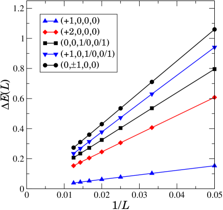
Figure 2: Plots of the low-lying energy gaps versus $1/L$ for $D=0.90$ $\lambda=1$. The states are labeled with the quantum numbers of the CFT (see text).

Moving downward with $D$ well into the Haldane phase up to $D=0.3,\,0.6$, in the $S_{\textrm{tot}}^{z}=0$ sector we observe besides a doublet state that we identify with the secondary states $\left(0,0,1/0,0/1\right)$, two clearly separated states that are the evolution of the $(0,\pm 1,0,0)$ doublet. This feature is evident in fig. 3 reporting the case $D=0.3$. At these values of $D$ the correlation length is sufficiently small, and we extrapolated the asymptotic values of the energy gap for both the soliton and the breather using the semi-phenomenological formula japar

$$\Delta E(L)=\Delta E(\infty)+\frac{A}{L}\exp\left(-\frac{L}{\xi^{\prime}}\right),$$ (9)

where the fitting parameter $\xi^{\prime}$ is expected to be proportional to the actual correlation length. We verified that eq. (9), fits better the data than other functions with different exponents of $1/L$. The extrapolated values for the breather gaps lay slightly above the continuum threshold, specifically we obtain $R=2.048$ at $D=0.6$ and $R=2.043$ at $D=0.3$. In addition we verified that also the lowest state in the $S_{\textrm{tot}}^{z}=2$ sector remains in the continuum in the thermodynamic limit.

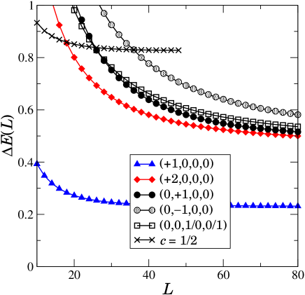
Figure 3: Plots of the low-lying energy gaps versus $L$ for $D=0.3$ at $\lambda=1$. States are still labeled as in fig. 2, except that here the states $(0,\pm 1,0,0)$ have split and grey circles represent the highest of the two. It is already possible to see the first excitation of the $c=1/2$ theory (crosses); this state appears incomplete because for $L\geq 50$ it lies outside the set of the DMRG-targeted states.

We pushed the analysis a little further for $D\geq 1.5$. As the correlation length is now sufficiently small we trust the data at $L=100$ without the help of any extrapolations. The result is that also in this regime $R>2$ so that there are no stable breathers. In agreement with what observed in feverati1998a ; feverati1998b , where the finite-size spectrum of the SGM is studied, the first excitation in the sector $S_{{\rm tot}}^{z}=0$ lies always above the soliton.

In summary, as far as the $K>1$ region is concerned, the numerical investigation allows to conclude that there are no soliton bound states both in the Haldane and in the large-$D$ phases.

3.2 $K<1$: Emergence of the breather

Let’s analyze now what happens on the $\lambda=2.59$ line, for which we have previously checked that $D_{{\rm c}}=2.30$ and $K=0.85$ on_c1_line . If we believe in the SGM as a faithful continuum theory of the low energy part of the model (1) we expect the spectrum to present a stable breather both in the Haldane and in the large-$D$ phases. According to the estimated $K$ the order of the CFT energy levels is the one reported in table 1 where we have shown the scaling dimensions $d^{\textrm{CFT}}=d_{mn}+r+\bar{r}$.

$d^{{\rm CFT}}$[$\times$ degeneracy]	$(m,n,r,\bar{r})$
0 [$\times$1]	(0,0,0,0)
$0.294\pm 0.003$ [$\times$2]	($\pm 1$,0,0,0)
$0.85\pm 0.01$ [$\times$2]	(0,$\pm 1$,0,0)
1 [$\times$2]	(0,0,1/0,0/1)
$1.18\pm 0.01$ [$\times$2]	($\pm 2$,0,0,0)
$1.29\pm 0.02$ [$\times$4]	($\pm 1$,0,1/0,0/1)

Table 1: Spectrum of scaling dimensions at the point ($\lambda=2.59$,$D_{{\rm c}}=2.30$), obtained from formula (6) where $K=0.85\pm 0.01$ on_c1_line .

As in the case $K>1$, we are interested in the soliton gap originating from the $\left(\pm 1,0,0,0\right)$ states and in the breather coming from the $\left(0,\pm 1,0,0\right)$ states.

The correlation length now decreases rather rapidly with $\left|D-D_{c}\right|$ so that we see the off-critical regime for $D$ quite close to the critical point for the system sizes at our disposal.

Inside the large-$D$ phase we selected eight points with $D$ ranging from 2.39 to 3. We have checked that the correlation length is indeed so small that we can use the data at $L=100$ without any finite-size scaling. The identification of the soliton and the breather states out of the DMRG spectrum is rather direct. Apart from a single point quite close to the critical line, the gap ratio $R$ is always less than two, as shown in fig. 4. This confirms the existence of an additional stable particle that we identify as the breather. Considering the non-monotonic behavior of the function $R\left(D\right)$, we can speculate whether the breather looses its stability for very large values of $D$. In the next section we will study this point by means of an analytical approach.

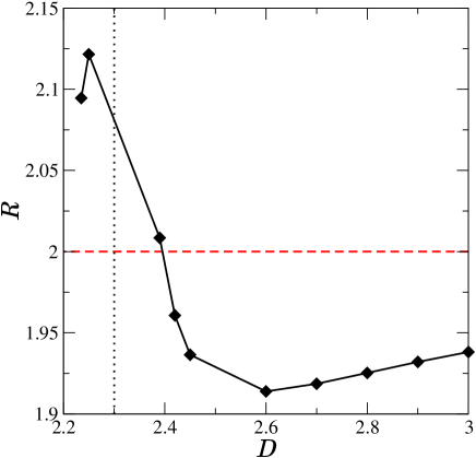
Figure 4: Plot of the ratio $R$ between the breather and the soliton energy gaps at $L=100$ as a function of $D$ for $\lambda=2.59$. The dashed horizontal line represents the continuum threshold while the dotted vertical line marks the critical point.

In the Haldane phase, which is very narrow here, we studied the points $D=2.2222,\,2.235,\,2.25$. The identification of the soliton and the breather is now complicated by the appearance of states which do not originate from the $c=1$ CFT. A typical numerical spectrum up to $L=100$ is shown in fig. 5. Following the states in the $S_{\textrm{tot}}^{z}=0$ sector, labelled by crosses, for smaller values of $D$ we observe that their gaps decrease and eventually vanish at the $c=1/2$ transition line whereas all the other states remain massive. For this reason we identify these states as excitations coming from the $c=1/2$ CFT. The doublet (triangles down) cannot be identified with the breather being twofold degenerate; it is probably a descendent ($r=0/1,\,\bar{r}=1/0$) of the first $c=1/2$ state. What we find is that, both at $D=2.25$ and at $D=2.235$, the breather lies above the two-soliton gap continuum, i.e. $R>2$. The point $D=2.2222$ lies on the “degeneracy-line” where the soliton gap is degenerate with the level originating from the first excitation of the $c=1/2$ theory. Now many states fall below the breather so that the latter can no longer be seen within the numerically available levels.

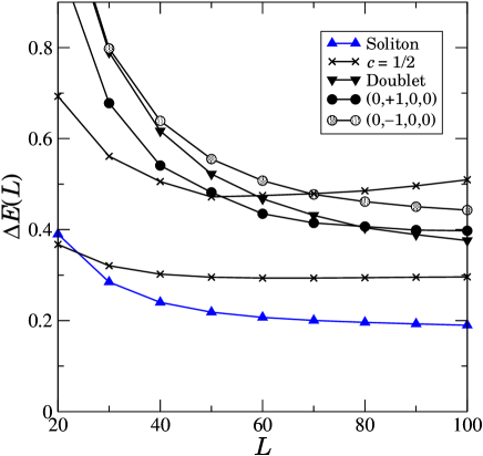
Figure 5: Typical low-lying spectrum in the Haldane phase for $K<1$ ($\lambda=2.59,\,D=2.235$).

4 Perturbation theory at large-$D$

From the data reported in fig. 4 one is led to separate the large-$D$ phase into two regions depending on the stability of the breather. However, the location of the curve $\lambda_{{\rm stab}}(D)$ separating the two regions is still vague: it starts from the $c=1$ H-D line at the point where $K=1$, close to $\lambda\simeq 2$, but we have no precise indications for larger values of $D$. In this region a perturbative analysis can be carried on. From the results quoted in orendac1999 it is known that bound states (at zero total momentum) do not exist for $\lambda=1$. Here we show that the presence of an Ising-like anisotropy $\lambda$ allows for a stabilization of breather states.

We start by treating the $D$-term as unperturbed Hamiltonian

$$H_{0}\equiv D\sum_{j=1}^{L}\left(S_{j}^{z}\right)^{2},$$ (10)

and the rest as small perturbation

$$V\equiv\sum_{j=1}^{L}\left\{\frac{1}{2}\left[S_{j}^{+}S_{j+1}^{-}+S_{j}^{-}S_{j+1}^{+}\right]+\lambda S_{j}^{z}S_{j+1}^{z}\right\}.$$

Both $H_{0}$ and $V$ commute separately with the total $z$-component of the spin, $S_{{\rm tot}}^{z}$, and with the total “spin-flip” (or “time-inversion”) operator $T=\exp({\rm i\pi}S_{{\rm tot}}^{y})$. However, $[S_{{\rm tot}}^{z},T]\neq 0$ and one can specify both quantum numbers for the energy eigenstates only in the sector $S_{{\rm tot}}^{z}=0$. The GS falls precisely in this sector and here we expect to find the breather. The soliton and the anti-soliton have $S_{{\rm tot}}^{z}=\pm 1$, but we can restrict to the soliton case $S_{{\rm tot}}^{z}=1$ since the anti-soliton state is simply obtained by applying $T$.

State	Energy	Degeneracy	Name
$|0_{1}\cdots 0_{L}\rangle$	$0$	1	GS
$|0_{1}\cdots+_{j}\cdots 0_{L}\rangle$	$D$	$L$	Soliton
$1\leq j\leq L$
$|0_{1}\cdots+_{j}\cdots-_{k}\cdots 0_{L}\rangle$	$2D$	$L\left(L-1\right)$	Breather
$1\leq j\neq k\leq L$

Table 2: Low energy states of the unperturbed Hamiltonian (10).

In table 2 we show the GS together with the first excited states for the unperturbed Hamiltonian (10). In this picture the “solitons” are completely degenerate and non-interacting so that the (soliton-antisoliton) “breather’s” energy is exactly twice that of the 1-particle states. As we switch on the interaction $V$, the GS energy becomes $E^{\left(0\right)}=-L/D+O\left(D^{-2}\right)$ up to second order in perturbation theory. The first excitations are no longer degenerate; they rather form a band, labelled by the lattice momentum $q$, $E_{q}^{\left(1\right)}=D+2\cos\left(q\right)+O\left(D^{-1}\right)$. Up to first order perturbation theory these 1-particle states form a continuum of two-particle scattering states whose upper and lower edges are given by the dashed lines in fig. 6. As a result of the interaction the soliton states may form bound state if their energy lies below the two-particle continuum. At first perturbative order the breather energy can be calculated using the Bethe-Ansatz approach; details can be found in Appendix A. The resulting breather states are indexed by the center-of-mass momentum $Q$. Acceptable states are those for which $\cos\left(Q/2\right)<\lambda/2$. This condition defines a characteristic wavenumber $Q^{\ast}$ above which the breather form a bound state with energy

$$E_{Q}^{\left(2\right)}=2D-\lambda-\frac{4}{\lambda}\cos\left(Q/2\right)+O\left(D^{-1}\right),\,\textrm{for}\,\,\left|Q\right|>Q^{\ast}.$$ (11)

Note that for $Q=\pi$ the bound state is always below the continuum with an energy shift $\delta E_{\pi}^{\left(2\right)}=-\lambda$. However with the DMRG we inspect the low-lying part of the spectrum, and in order to find a stable bound state, that will be identified with the breather, we must examine the minimum of the continuum at $Q=0$. In this case the bound states emerges from the continuum only for $\lambda>2$ with an energy shift $\delta E_{0}^{\left(2\right)}=-\lambda-4/\lambda$. The mechanism is illustrated in fig. 6 for some values of $\lambda$. Interestingly enough, the mass ratio $R=\Delta E_{{\rm b}}(\infty)/\Delta E_{{\rm s}}(\infty)$ now reads:

$$R=\frac{E_{0}^{\left(2\right)}}{E_{\pi}^{\left(1\right)}}=2-\frac{1}{\lambda}\frac{\left(\lambda-2\right)^{2}}{\left(D-2\right)}.$$ (12)

This equation is valid for $\lambda>2$, meaning that the stability boundary is $\lambda_{{\rm stab}}(D)=2$ independent of $D$. This result is consistent with the stability criterion provided by the SGM: $K=1$ just for $\lambda\sim 2$ on_c1_line . In addition the ratio converges to $R=2$ from below in agreement with fig. 4. The first-order approximation is also quantitatively good in comparison to the DMRG values as shown by the example in fig. 7.

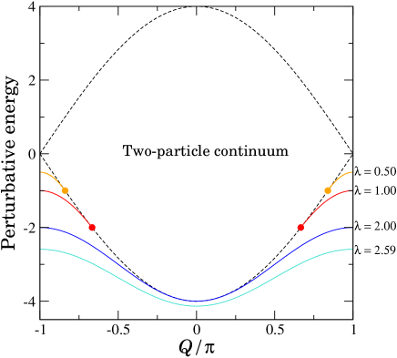
Figure 6: Bound states (full lines) and continuum (region enclosed by dashed lines) for the values of $\lambda$ indicated on the right. Full dots mark the wavenumbers $Q^{*}$ where the bound state starts to detach from the continuum when $\lambda<2$.

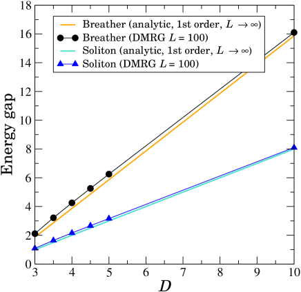
Figure 7: Results of first-order perturbation theory vs DMRG data in the large-$D$ phase at $\lambda=2.59$.

5 Discussion of the results and conclusions

Motivated by field-theoretic predictions, in this paper we have investigated the stability of massive excitations (soliton, ant-isoliton and breathers) that are present in the large-$D$ and Haldane phases of the anisotropic spin-1 Heisenberg chain with both Ising-like and single-ion anisotropy.

In excellent agreement with the SGM that is supposed to describe the continum limit of the lattice model in the vicinity of the H-D critical line, we have provided both numerical and analytical results supporting the existence of a stable breather in the large-$D$ phase of the model (1) in the region with $\lambda>2$.

On the contrary, as far as the Haldane phase is concerned, our best estimates do not show other stable states in addition to the three particles that form the Haldane triplet at the isotropic Heisenberg point. This is at variance with what we would expect from the SGM, indicating that the latter is probably not sufficient to describe the effective interaction when there is an underlying topological order as the one found in the Haldane phase kennedy92 . Indeed in this phase we may expect that we cannot neglect the effects of an interaction between the states coming from the $c=1$ CFT describing the H-D critical line and those pertaining to the $c=1/2$ CFT describing the H-I transition.

It is interesting to speculate whether this excitation can be observed in real materials. The so called NENC has the advantage of having a large single-ion anisotropy $D\simeq 7.5$ but $\lambda=1$ in this compound. On the other hand large Ising anisotropies are present in some spin-1/2 materials (e.g. $\textrm{CsCoCl}_{3}$ and $\textrm{CsCoBr}_{3}$; see asano2002 and references therein). Interestingly enough, differently from existing experiments the mechanism proposed here to observe breather states does not require the presence of external magnetic fields.

Appendix A

In this appendix we show how to evaluate the first order correction of the second energy level in $S_{\textrm{tot}}^{z}=0$. The unperturbed states are

$$|u_{j,k}^{\left(2\right)}\rangle=|0_{1}\cdots+_{j}\cdots-_{k}\cdots 0_{L}\rangle,\,\,j\neq k$$

and we need the eigenvalues of the matrix $\langle u_{l,m}^{\left(2\right)}|V|u_{j,k}^{\left(2\right)}\rangle$ with $j\neq k$ and $l\neq m$. We write the –unnormalized– eigenfunction as

$$|\psi^{\left(2\right)}\rangle=\sum_{j,k}f_{j,k}|u_{j,k}^{\left(2\right)}\rangle.$$

The states can be classified according to the eigenvalue of $T$:

$$T|\psi^{\left(2\right)}\rangle=\tau|\psi^{\left(2\right)}\rangle,\;\tau=\pm 1\;\Rightarrow f_{kj}=\tau f_{jk}.$$

In terms of the coefficients $f_{jk}$ the eigenvalue equation reads:

$$(1-\delta_{jk})\left[f_{j+1,k}+f_{j,k-1}+f_{j-1,k}+f_{j,k+1}\right]\\ -\lambda f_{jk}\left(\delta_{j,k+1}+\delta_{j,k-1}\right)=\delta E^{\left(2\right)}f_{jk}.$$ (13)

Note that we have put the term $(1-\delta_{jk})$ in the left-hand side for compatibility with the requirement $f_{jj}=0$. Now, eq. (13) is an eigenvalue equation in a $L(L-1)$-dimensional space. It is actually much more simple to express the amplitudes using relative and center-of-mass coordinates: $r=j-k$ and $\rho=(j+k)/2$. From now on we will follow closely the approach used in Mattis’ book mat (sec. 5.3) for the bound states of magnons in Heisenberg ferromagnets. Consider the wave function:

$$f_{jk}=\exp\left({\rm iQ\rho}\right)F(r),\;F(r)=\sum_{p}f(p)\exp\left({\rm i}pr\right),$$ (14)

where $Q$ and $p$ denote the total and relative momenta respectively, both ranging in $(-\pi,\pi]$. The eigenvalue of $T$ reflects directly in the parity of the Fourier transform: $f(-p)=\tau f(p)$, while the constraint $f_{jj}=0$ becomes $F(0)=\sum_{p}f(p)=0$. When (14) is plugged into (13) a common factor $\exp\left({\rm iQ\rho}\right)$ can be simplified from both members and we are left with the simpler equation:

$$(1-\delta_{r,0})\cos\left(\frac{Q}{2}\right)\left[F(r+1)+F(r-1)\right]\\ -\lambda F(r)(\delta_{r,1}+\delta_{r,-1})=\delta E^{\left(2\right)}F(r),$$ (15)

that appears as a finite-differences Schrödinger equation with a $\delta$-potential at $r=\pm 1$. From now on we fix $\tau=1$; the procedure for $\tau=-1$ is analogous and the conclusions are exactely the same. In momentum space eq. (15) becomes:

$$4f(p)\cos\left(\frac{Q}{2}\right)\cos p-\frac{2}{L}\left[\lambda\cos p+2\cos(\frac{Q}{2})\right]\\ \times\sum_{p^{\prime}}f(p^{\prime}){\rm cos}p^{\prime}=\delta E^{\left(2\right)}f(p).$$ (16)

Were it not for the $\lambda$-term, the spectrum of eigenvalues $\delta E^{\left(2\right)}(Q,p)$ would be identical to that of two non-interacting soliton and anti-soliton with energy $(2\cos q+2\cos q^{\prime})=4\cos(Q/2)\cos p$ with $Q=q+q^{\prime}$ and $p=(q-q^{\prime})/2$. In the thermodynamic limit $L\rightarrow\infty$ at a given $Q$ these form a continuum $-4\cos(Q/2)\leq\delta E_{{\rm cont}}\leq 4\cos(Q/2)$. Hence, defining ${\cal E}\equiv\delta E^{\left(2\right)}/4\cos(Q/2)$, the bound states will be searched in the region $|{\cal E}|>1$. Eq. (16) can be solved formally as:

$$f(p)=\Gamma\frac{C\cos p+1}{\cos p-{\cal E}},$$ (17)

where $C=\lambda/[2\cos(Q/2)]$ and

$$\Gamma\equiv\frac{1}{2\pi}\int_{-\pi}^{\pi}{\rm d}p\>f(p)\cos p$$ (18)

Now, re-inserting (17) into (18), self-consistency demands that either $\Gamma=0$ or:

$$1=\frac{1}{2\pi}\int_{-\pi}^{\pi}{\rm d}p\>\cos p\frac{C\cos p+1}{\cos p-{\cal E}}.$$

Evaluating the integral the energy equation becomes:

$$\sqrt{\frac{{\cal E}^{2}-1}{|{\cal E}|^{2}}}=\frac{C{\cal E}+1}{C{\cal E}}.$$

With $\lambda>0$ one has a solution either for ${\cal E}>1$ or for ${\cal E}\leq\min(-1,-C^{-1})$. Under these conditions the solution reads ${\cal E}=-(1+C^{2})/2C$. The condition $\mathcal{E}\leq-C^{-1}$ should be imposed for $C<1$ but then the requirement would be $C\geq 1$. So we can only accept the case $C>1$ for which $\mathcal{E}<-1$ is always fullfilled. It can be also seen that $\sum_{p}f(p)=0$ is automatically satisfied if we build $f(p)$ from eq. (17). The restriction $C>1$ can be re-expressed as $\cos(Q/2)<\lambda/2$ and defines a characteristic wavenumber $Q^{*}$ above which the bound state with energy

$$\delta E^{\left(2\right)}(Q)=-\lambda-\frac{4}{\lambda}\cos^{2}\left(\frac{Q}{2}\right),\;|Q|\geq Q^{*}$$

emerges from the continuum. This is precisely the result of eq. (11).

References

- (1) F.D.M. Haldane, Phys. Rev. Lett. 50, 1153 (1983)
- (2) A. Auerbach, Interacting electrons and quantum magnetism (Springer-Verlag, 1994)
- (3) T. Asano, H. Nojiri, Y. Inagaki, J.P. Boucher, T. Sakon, Y. Ajiro, M. Motokawa, Phys. Rev. Lett. 84, 5880 (2000)
- (4) M. Kenzelmann, Y. Chen, C.L. Broholm, D.H. Reich, Y. Qiu, Phys. Rev. Lett. 93, 017204 (2004)
- (5) S. Zvyagin, A.K. Kolezhuk, J. Krzystek, R. Feyerherm, Phys. Rev. Lett. 93, 027201 (2004)
- (6) C. Degli Esposti Boschi, E. Ercolessi, F. Ortolani, M. Roncaglia, Eur. Phys. J. B 35, 465 (2003)
- (7) W. Chen, K. Hida, B.C. Sanctuary, Phys. Rev. B 67, 104401 (2003)
- (8) M. den Nijs, K. Rommelse, Phys. Rev. B 40, 4709 (1989)
- (9) R. Botet, R. Julien, M. Kolb, Phys. Rev. B 28, 3914 (1983)
- (10) S. Pasini, Ph.D. thesis, Università di Bologna (2006)
- (11) S. Lukyanov, A. Zamolodchikov, Nucl. Phys. B 493, 571 (1997)
- (12) U. Schollwöck, Rev. Mod. Phys. 77, 259 (2005)
- (13) C. Degli Esposti Boschi, F. Ortolani, Eur. Phys. J. B 41, 503 (2004)
- (14) X. Wang, Mod. Phys. Lett. B 14, 327 (2000)
- (15) O. Legeza, G. Fáth, Phys. Rev. B 53, 14349 (1996)
- (16) G. Bouzerar, A.P. Kampf, G.I. Japaridze, Phys. Rev. B 58, 3117 (1998)
- (17) G. Feverati, F. Ravanini, G. Takács, Phys. Lett. B 430, 264 (1998)
- (18) G. Feverati, F. Ravanini, G. Takács, Phys. Lett. B 444, 442 (1998)
- (19) M. Orendác, S. Zvyagin, A. Orendácová, M. Sieling, B. Lüthi, A. Feher, M.W. Meisel, Phys. Rev. B 60, 4170 (1999)
- (20) T. Kennedy, H. Tasaki, Commun. Math. Phys. 147, 431 (1992)
- (21) T. Asano, H. Nojiri, Y. Inagaki, Y. Ajiro, L.P. Regnault, J.P. Boucher, cond-mat/0201298
- (22) D.C. Mattis, The theory of magnetism I: Static and dynamics (Springer-Verlag, 1988)