Slave-boson approach to the metallic stripe phases with large unit cells

Abstract

Using a rotationally invariant version of the slave-boson approach in spin space we analyze the stability of stripe phases with large unit cells in the two-dimensional Hubbard model. This approach allows one to treat strong electron correlations in the stripe phases relevant in the low doping regime, and gives results representative of the thermodynamic limit. Thereby we resolve the longstanding controversy concerning the role played by the kinetic energy in stripe phases. While the transverse hopping across the domain walls yields the largest kinetic energy gain in the case of the insulating stripes with one hole per site, the holes propagating along the domain walls stabilize the metallic vertical stripes with one hole per two sites, as observed in the cuprates. We also show that a finite next-nearest neighbor hopping $t^{\prime}$ can tip the energy balance between the filled diagonal and half-filled vertical stripes, which might explain a change in the spatial orientation of stripes observed in the high $T_{c}$ cuprates at the doping $x\simeq 1/16$.

I Introduction

The experimentally established existence of nanoscale charge order phenomena in transition metal oxides continues to attract much attention. In particular, phase separation, manifesting itself in formation of nonmagnetic one-dimensional (1D) domain walls which separate the antiferromagnetic (AF) domains with opposite phases, has been proposed to be responsible for unusual properties of the high $T_{c}$ copper oxide superconductors.Kiv03 Moreover, taking into account that magnetic excitation spectra have been found to be similar among various high $T_{c}$ cuprates, the knowledge of the spatial distribution of holes in the CuO₂ planes might be a first step towards microscopic understanding mechanism of the superconductivity itself.Lee06 Indeed, the most prominent feature of the spin excitations in YBa₂Cu₃O_6+δ (YBCO) is the resonance that occurs at the AF wavevector ${\bf Q}=(\pi,\pi)$ and at the energy of 41 meV in the case of optimal doping while for lower energies incommensurate (IC) magnetic peaks emerge. Hay04 In contrast, for a long time it was thought that La_2-xSr_xCuO₄ (LSCO) does not show the resonance and that the corresponding IC fluctuations are dispersionless. However, recent high-resolution neutron scattering studies on optimally doped sample have revealed that in fact the magnetic excitations are dispersive and quite similar to those of YBCO. Chr04 Moreover, the overall evolution of the magnetic scattering with energy in La_2-xBa_xCuO₄ (LBCO) also resembles the one found in YBCO. Tra04 Altogether, the common low-energy excitations imply that the spin dynamics in doped copper oxide superconductors has the same origin. Remarkably, the observed spectra might be consistently explained in terms of fluctuating stripes suggesting that the stripe instability is a universal phenomenon of all cuprates and thus it might be indeed regarded as relevant for the superconductivity.Sei05

Historically, the first compelling evidence for both magnetic and charge order in the cuprates, was accomplished in a neodymium codoped compound La_1.6-xNd_0.4Sr_xCuO₄ (Nd-LSCO). Indeed, around hole doping $x=1/8$, Tranquada et al. Tra95Nd found that elastic neutron scattering is characterized by magnetic peaks at the wave vectors ${\bf Q}=\pi(1\pm 2\epsilon,1)$ and ${\bf Q}=\pi(1,1\pm 2\epsilon)$. Such positions of the peaks corresponds to equally probable modulations along one of two equivalent lattice directions $x$ and $y$, to which we refer as horizontal and vertical stripes, respectively. Moreover, inspired by the pioneering Hartree-Fock (HF) studies suggesting that the staggered magnetization undergoes a phase shift of $\pi$ at the charge domain wall (DW), Zaa89 the authors found additional Bragg peaks displaced symmetrically by $\pm 4\pi\epsilon$ around the $\Gamma=(0,0)$ point, precisely at the position expected for charge modulation. Recently, the same geometry for static IC magnetic and charge peaks has been reportedFuj04 in LBCO with $x=1/8$. In fact, neutrons do not detect charge directly but instead they are sensitive to nuclear displacements induced by the charge modulation. Therefore, a very recent resonant soft X-ray scattering study of the charge order in LBCO at the same doping is of a particular great value being a more direct evidence of charge modulation. These studies have yielded an estimate for the number of holes per DW to be 0.59, very close to the expected from neutron scattering experiments value 0.5. It corresponds to the so-called half-filled stripes, as they are characterized by the filling of one doped hole per two atoms along the DWs. Abb05 Remarkably, at this particular doping, both compounds exhibit a deep minimum in the doping dependence of $T_{c}$, suggesting a strong competition between the static stripe order and the superconductivity.Moo88

Conversely, the large drop in $T_{c}$ at $x=1/8$ is not observed in LSCO, even though inelastic neutron scattering experiments in the superconducting regime of $x\geq 0.06$ have revealed the presence of magnetic peaks at the same IC positions as in Nd-LSCO and LBCO. Moreover, Yamada et al.Yam98 established a remarkably simple relation $\epsilon\simeq x$ for $0.06\leq x\leq 0.125$ with a lock-in effect at $\epsilon\simeq 1/8$ for larger $x$. This means that increasing doping reduces the distance $d=1/2x$ between the half-filled stripes. Hence, it appears that such a stripe order is compatible with the superconductivity, which is particularly pronounced when the spin correlations remain purely dynamic. However, the superconducting state may also coexist with static stripe order,Tra97 but then the value of $T_{c}$ is strongly reduced. This conjecture is strongly supported by inelastic neutron scattering experiments on YBCO, which have also established the presence of IC vertical/horizontal spin fluctuations throughout the entire superconducting regime of YBCO. Dai01 Moreover, for $\delta=0.35$, apart from spin fluctuations, Mook et al. Moo02 have found an IC charge order consistent with the vertical/horizontal stripes.

In contrast, in the insulating spin-glass regime of LSCO $x<0.06$, quasielastic neutron scattering experiments with the main weight at zero frequency demonstrate that IC magnetic peaks are located at the wave vector $\textbf{Q}=\pi(1\pm\sqrt{2}\epsilon,1\pm\sqrt{2}\epsilon)$. Wak99 This phenomenon has often been interpreted as the existence of static diagonal stripes, even though no signatures of any charge modulation were observed. In spite of the change in spin modulation from the diagonal to vertical/horizontal one at the doping $x\simeq 0.06$, $\epsilon$ follows $x$ reasonably well over the entire low doping range $0.03\leq x\leq 0.125$. Moreover, the same type of the diagonal IC spin modulation has been discovered in Nd-LSCO at $x=0.05$, Wak01 indicating that while the vertical/horizontal spin-density modulation, accompanied by the charge modulation, might be regarded as a generic property of the superconducting regime, the diagonal orientation of the magnetic domains is common for the lightly Sr-doped insulating systems. Finally, in the narrow range of low doping $0.02\leq x\leq 0.024$, IC magnetic peaks in LSCO are observed at the wave vector $\textbf{Q}=\pi(1\pm\epsilon,1\pm\epsilon)$, Mat00 just as in the insulating La_2-xSr_xNiO₄ (LSNO) compound. Sac95 In this case, the spacing between stripes is equal to $d=1/x$; such structures with the filling of one doped hole per one atom in the DW correspond to the so-called filled stripes.

The intriguing competition between vertical and diagonal stripes has been already noticed in the early mean-field studies. Zaa89 Indeed, it has been found that the vertical stripes were favored for $U/t\lesssim 4$ whereas the diagonal DWs were formed at a stronger Coulomb repulsion. Unfortunately, these studies predicted the filled stripes in the ground state. A general feature of such instability is a gap/pseudogap precisely on the Fermi surface. As a result, charge transport is not possible in idealized filled stripes. In contrast, the ground state energy half-filled stripes observed in the cuprates, have been found in a few methods which go beyond the Hartree-Fock approximation (HFA), such as: density matrix renormalization group,Whi98 variational local ansatz approximation,Gor99 Exact Diagonalization (ED) of finite clusters, Toh99 analytical approaches based on variational trial wave function within the string picture, Che02 ; Wro00 dynamical mean field theory, Fle00 cluster perturbation theory, Zac00 and Quantum Monte Carlo (QMC) simulations, Bec01 indicating the crucial role of local electron correlations in stabilizing these structures. Indeed, while the HF method is well suited to compare the energies of different types of magnetically ordered phases in the limit of large on-site Coulomb interaction $U\to\infty$, where it gives the same asymptotic behavior as the SBA or the Gutzwiller ansatz,Ole89 it is crucial to use a better approach than the HFA at intermediate $U$, particularly when magnetic polarization of some sites is missing.

A good starting point for a proper approximate treatment of strong correlations is the representation of the Hubbard model in terms of auxiliary fermions and bosons. Kot86 The slave-boson approximation (SBA) has been applied successfully to a whole range of problems and is known to provide a realistic mean-field description of strongly correlated systems. It is quite encouraging that the ground state phase diagram obtained using spin-rotation-invariant (SRI) slave-boson representation of the two-dimensional (2D) Hubbard model with homogeneous spiral, AF order, ferromagnetic (FM), and paramagnetic (PM) phases shows a good agreement both with QMC simulations and the ED method. Fre92sp The slave-boson (SB) method was also used to investigate magnetic and charge correlations of the $t$-$t^{\prime}$-U model, Fre98 the ground state of the Anderson lattice model, Mol93 and systems with orbital degeneracy. Has97 Moreover, the unrestricted slave-boson formalism has turned out to be a powerful tool in description of inhomogeneous states, even though in the absence of a finite long-range Coulomb repulsion, completely filled diagonal stripes (FDS) were found to be more stable than the half-filled vertical stripes (HVS), suggesting that a pure Hubbard model might be insufficient to capture the physics in the cuprates. Sei98 ; Sei98V

Another possible extension could involve an inclusion of the next-nearest neighbor hopping term $t^{\prime}$. There are several experimental and theoretical studies suggesting the presence of a finite $t^{\prime}$ in the cuprates. Indeed, topology of the Fermi surface seen by angle-resolved photoemission spectroscopy Dam03 and the asymmetry of the phase diagrams of the hole- and electron-doped cuprates can be understood only by introducing $t^{\prime}$. Toh04 It also offers an explanation for the variation of $T_{c}$ among different families of hole-doped cuprates.Pav01 ; Pre05 Moreover, ED studies have shown that while the $d$-wave superconductivity correlation is slightly suppressed by $t^{\prime}$ in underdoped regions, it is substantially enhanced in the optimally doped and overdoped regions, indicating that $t^{\prime}$ is of great importance for the pairing instability.Shi04

Finally, Seibold and Lorenzana have foundSei04 that a finite $t^{\prime}$ strongly affects the optimal filling of the vertical stripes and consequently favors partially filled configurations in the SBA. Unfortunately, restrictions due to the cluster size, have not let the authors to reach an unambiguous conclusion concerning a crossover towards the FDS at low doping. Motivated by this result, we have investigated recently the relative stability between the latter and the HVS with the symmetry lowered by a period quadrupling due to on-wall spin-density wave. Using the self-consistent HFA, one finds that a negative ratio of the next-to nearest neighbor hopping ($t^{\prime}/t<0$) expels holes from the AF domains and reinforces the stripe order. Therefore, the half-filled stripes not only accommodate holes but also redistribute them so that the kinetic energy is gained, and these stripes take over in the regime of $t^{\prime}/t\simeq-0.3$ appropriate for YBCO. Rac06

The purpose of this paper it to investigate the stability of stripe phases at low doping and to resolve the longstanding controversy concerning the role of the kinetic energy in the formation of stripes. Domain walls can be viewed as topological defects in the AF phase, which confine the holes to 1D regions, while a crossover to a 2D system occurs when the stripes melt.Cas01 This leads in a natural way to the picture of 1D composite excitations,Che02 which contribute to the kinetic energy by the hole motion along DWs. In contrast, in the early HF studies it was demonstrated that the stripes are stabilized by the kinetic energy increments due to the bonds connecting the domain wall with the neighboring sites of AF domains. Zaa96

The rest of the paper is as follows. In Sec. II we shortly review the SRI slave-boson representation of the Hubbard model and introduce reciprocal space formalism, based on the stripe periodicity, which provides a possibility to perform calculations on larger ($128\times$128) clusters than those studied in Ref. Sei04, . Therefore, our approach eliminates to a large extent the role of finite-size effects, as we show it in Sec. II.4. Further, in Sec. III we investigate the stability of the already mentioned FDS and HVS as well as of the filled vertical stripes (FVS) and half-filled diagonal stripes (HDS) at the two representative doping levels $x=1/8$ and $x=1/16$. For stable structures we compare the charge, spin, and double occupancy profiles obtained in the SBA with the ones obtained in the HFA. We also analyze in detail kinetic and magnetic energy contribution as well as discuss the shape of the density of states (DOS). The effect of a finite next-nearest neighbor hopping $t^{\prime}$ on the stripe stability and induced by it conspicuous changes in the band structure are presented in Sec. IV. Finally, in Sec. V we present a short summary and general conclusions.

II Formalism

II.1 Rotationally invariant slave-boson method

In this paper we study the 2D Hubbard model,

$$H=-\sum_{ij,\sigma}t_{ij}c^{{\dagger}}_{i\sigma}c_{j\sigma}+U\sum_{i}n_{i\uparrow}n_{i\downarrow},$$ (1)

where the electron hopping $t_{ij}$ is $t$ on the bonds connecting the nearest neighbor sites $\langle ij\rangle$ and $t^{\prime}$ between next-nearest neighbor sites, while $U$ stands for the on-site Coulomb interaction. Our study is based on the spin-rotation invariant formulation of the Kotliar and RuckensteinKot86 SB representation of the Hubbard model,Fre92 ; Fre01 in which one enlarges the Hilbert space of the Hamiltonian (1) by introducing auxiliary boson operators: $e_{i}$ and $d_{i}$, as well as a scalar $p_{i0}$ and a vector $\textbf{p}_{i}=(p_{i1},p_{i2},p_{i3})$ bosonic field at each site. The former operators act as projection operators on empty and doubly occupied sites, while the latter describe the spin and charge degrees of freedom in the singly occupied subspace.

The main advantage of such a representation is that the actual electron configuration is controlled by the bosons and one can thus write the Hubbard interaction as a bosonic occupation number operator. In contrast, the operator for the kinetic energy becomes more involved since the motion of a physical electron changes boson occupation numbers on both lattice sites involved in the hopping process. Hence, in terms of the above SB operators, the Hubbard model (1) takes the form,

$$H_{SB}=-\sum_{ij}\sum_{\sigma\sigma^{\prime}\sigma^{\prime\prime}}t_{ij}z^{{\dagger}}_{i\sigma\sigma^{\prime}}f^{{\dagger}}_{i\sigma^{\prime}}f_{j\sigma^{\prime\prime}}z_{j\sigma^{\prime\prime}\sigma}+U\sum_{i}d^{{\dagger}}_{i}d_{i},$$ (2)

where $\underline{z}_{i}$ are $2\times 2$ matrices in spin space which depend on the actual configuration of the boson fields, as explained in Ref. Zim97, . These matrices are constructed in such a way that the correct mean-field result in the noninteracting limit (at $U=0$) is recovered. Additionally, the SB operators have to fulfill the following constraints at each site,

$$e_{i}^{{\dagger}}e_{i}+d_{i}^{{\dagger}}d_{i}+\sum_{\mu}p_{i\mu}^{{\dagger}}p_{i\mu}=1,$$ (3)

$$2d_{i}^{{\dagger}}d_{i}+\sum_{\mu}p_{i\mu}^{{\dagger}}p_{i\mu}=\sum_{\sigma}f_{i\sigma}^{{\dagger}}f_{i\sigma},$$ (4)

$$p_{0i}^{{\dagger}}\textbf{p}_{i}+\textbf{p}_{i}^{{\dagger}}p_{0i}-i\textbf{p}_{i}^{{\dagger}}\times\textbf{p}_{i}=\sum_{\sigma\sigma^{\prime}}\boldsymbol{\tau}_{\sigma\sigma^{\prime}}f_{i\sigma^{\prime}}^{{\dagger}}f_{i\sigma}.$$ (5)

They are enforced by corresponding Lagrange multipliers in the action, and one obtains a path integral representation of the Hubbard model. Owing to the gauge symmetry group of the action, the phase of five of the six bosonic fields can be gauged away.Fre92 These fields can be handled in the Cartesian gauge, or in the radial gauge. Fre01 In the following we handle the action in the Cartesian gauge at saddle-point level (in the SBA). This procedure is exact in the large degeneracy limit.Fre92 ; Flo02 Comparison of ground state energies with data resulting from numerical simulations show very good agreement.Fre91 ; Fre92sp

Since homogeneous AF phases turned out to be unstable with respect to spiral phases,Fre91 one may anticipate that a similar effect will take place in stripe phases. Therefore, the present rotationally invariant formalism opens a possibility of studying also more general structures which we postpone to future studies. Here we will limit ourselves to noncanted states which are locally stable, as checked in a few representative cases.

II.2 Reciprocal space approach for stripe phases

In order to obtain unbiased results for stripe phases one should carry out calculations on large clusters. So far, such calculations were usually performed in real space to address directly inequivalent sites in the stripe unit cell. However, an efficient approach may be constructed by making use of the periodicity of a stripe phase which allows one to cover the entire lattice by small unit cells. Indeed, each position vector $\textbf{R}_{i}$ of an arbitrary atom can be decomposed into a sum involving certain periodicity vectors $\textbf{g}_{1}$ and $\textbf{g}_{2}$, and a vector $\boldsymbol{\delta}_{M}$ labeling all inequivalent sites $i$ within the unit cell:

$$\textbf{R}_{i}=n\textbf{g}_{1}+m\textbf{g}_{2}+\boldsymbol{\delta}_{M},$$ (6)

with integer $\{n,m\}$. Accordingly the covering of the Brillouin zone spanned by the wave vector k is achieved by the decomposition:

$$\textbf{k}=\textbf{K}+\textbf{G},$$ (7)

with G belonging to a set of wave vectors representative of the periodicity of the structure of interest.Asc76 For a stripe phase with vertical domain walls separated by $d=4$ lattice spacings, as shown in Fig. 1(a), the magnetic unit cell consists of a row of eight atoms perpendicular to the stripes. One immediately finds two periodicity vectors $\textbf{g}_{1}=\bigl{(}4,1\bigr{)}$ and $\textbf{g}_{2}=\bigl{(}0,2\bigr{)}$. In this case the set of vectors G satisfying $\exp\{i\textbf{g}_{(1,2)}\cdot\textbf{G}\}=1$ is given by

$$\textbf{G}_{1}^{(l)}=\frac{2\pi}{8}(2l,0),\qquad\textbf{G}_{2}^{(l)}=\frac{2\pi}{8}\bigl{(}2l+1,4\bigr{)},$$ (8)

with $0\leq l\leq 3$.

A second example is a diagonal stripe phase depicted in Fig. 1(b). Again, considering the periodicity of this phase, one finds the magnetic unit cell consisting of a row of eight atoms along the $x$-direction. However, the periodicity vectors are now given by $\textbf{g}_{1}=(1,1)$ and $\textbf{g}_{2}=(4,-4)$. Accordingly one finds for G:

$$\textbf{G}_{1}=(0,0),\qquad\textbf{G}_{2}^{(l)}=\frac{2\pi}{8}(l,8-l),$$ (9)

with $1\leq l\leq 7$.

Figure 1: Symmetry properties of stripe phases: (a) the vertical stripe phase — its unit cell with two periodicity vectors: $\textbf{g}_{1}=\bigl{(}4,1\bigr{)}$ and $\textbf{g}_{2}=\bigl{(}0,2\bigr{)}$; (b) the diagonal stripe phase — its unit cell with two periodicity vectors: $\textbf{g}_{1}=\bigl{(}1,1\bigr{)}$ and $\textbf{g}_{2}=\bigl{(}4,-4\bigr{)}$.

In both cases the vectors K in Eq. (7) are spanning the rectangle $[0,2\pi/8]\times[0,2\pi]$. The extension to other stripe phases is straightforward. Using the above procedure, the fermionic contribution to the action in the momentum representation is given by:

$${\mathcal{S}}_{f}\!=\!\int_{0}^{\beta}\!d\tau\sum_{\textbf{K}\textbf{G}\textbf{G}^{\prime}}\sum_{\sigma\sigma^{\prime}}f_{\textbf{K}+\textbf{G},\sigma}^{{\dagger}}(\tau)M_{\textbf{GG}^{\prime}}^{\sigma\sigma^{\prime}}(\textbf{K},\tau)f_{\textbf{K}+\textbf{G}^{\prime},\sigma^{\prime}}(\tau),$$ (10)

with,

$$M_{\textbf{GG}^{\prime}}^{\sigma\sigma^{\prime}}(\textbf{K},\tau) =(\partial_{\tau}-\mu)\delta_{\sigma\sigma^{\prime}}\delta_{\boldsymbol{G}\boldsymbol{G}^{\prime}}+\frac{1}{L}\sum_{\boldsymbol{\delta}_{M}}e^{-i(\boldsymbol{G}-\boldsymbol{G}^{\prime})\boldsymbol{\delta}_{M}}$$

$$\hskip-28.45274pt\times\Bigl{[}\beta_{0\boldsymbol{\delta}_{M}}(\tau)\delta_{\sigma\sigma^{\prime}}+\boldsymbol{\beta}_{\boldsymbol{\delta}_{M}}(\tau)\cdot\boldsymbol{\tau}_{\sigma\sigma^{\prime}}$$

$$\hskip-28.45274pt-\sum_{\boldsymbol{\delta}}t_{\boldsymbol{\delta}_{M},\boldsymbol{\delta}_{M}+\boldsymbol{\delta}}e^{i(\boldsymbol{K}+\boldsymbol{G}^{\prime})\boldsymbol{\delta}}\left(z_{\boldsymbol{\delta}_{M}+\boldsymbol{\delta}}(\tau)z_{\boldsymbol{\delta}_{M}}^{{\dagger}}(\tau)\right)^{T}_{\sigma\sigma^{\prime}}\Bigl{]}.$$ (11)

Here $L$ is the number of atoms in the unit cell so that the ratio $N/L$ gives the number of unit cells needed to cover a whole cluster with $N$ sites, $\partial_{\tau}$ is an imaginary time derivative, and $\mu$ is the chemical potential. The quantities $\beta_{0}$ and $\boldsymbol{\beta}$ are the Lagrange multipliers enforcing the constraints given in Eq. (4) and Eq. (5), respectively.

Hence, we have reduced the fermionic matrix $M_{\textbf{kk}^{\prime}}^{\sigma\sigma^{\prime}}$ down to decoupled blocks labeled by K. This procedure gives a considerable time gain during numerical calculations. While the usual workload in a diagonalization algorithm is $\sim N^{3}$ (see Ref. Pre96, ), the number of operations needed for diagonalization of $N/L$ smaller matrices is only $\sim\frac{N}{L}\cdot L^{3}=NL^{2}$. This means that the symmetry reduction makes a tremendous simplification and the time needed for numerical calculations is reduced by a factor $\left(N/L\right)^{2}$ as compared to a straightforward ’brute force’ diagonalization of an $N\times N$ matrix, which is necessary when the computations are performed in real space.

II.3 Mean-field approximation

In Secs. III and IV we present solutions for the stripe phases obtained within the SB mean-field approximation in which one replaces the Bose fields and the Lagrange multipliers by their time-independent averages. Hence, the free energy found at the temperature $T$ follows as, Fre92sp

$$F =\frac{1}{L}\Bigl{\{}\sum_{l}\bigl{[}\alpha_{l}(e^{2}_{l}+p_{0l}^{2}+p_{l}^{2}+d_{l}^{2}-1)$$

$$-\beta_{0l}(p_{0l}^{2}+p_{l}^{2}+2d_{l}^{2})+Ud_{l}^{2}-2\boldsymbol{\beta}_{l}\cdot\textbf{p}_{l}p_{0l}\bigr{]}$$

$$-\frac{1}{\beta}\sum_{\textbf{q}\sigma}\ln\bigl{(}1+e^{-\beta\varepsilon_{\textbf{q}\sigma}}\bigr{)}+\mu N_{el}\Bigr{\}},$$ (12)

with $\beta=1/k_{B}T$, $\varepsilon_{\textbf{q}\sigma}$ standing for the eigenmodes of the fermionic matrix (11), and $N_{el}$ corresponding to the total number of particles. The equilibrium values of the classical field amplitudes are determined from the saddle-point equations in which the partial derivatives are taken with respect to three Lagrange multipliers enforcing the constraints (3)–(5), as well as to the four SB fields $p_{0l}$, $p_{l}$, $e_{l}$, and $d_{l}$, for each inequivalent site $l=(l_{x},l_{y})$ within the elementary stripe unit cell. The saddle-point equations are solved using the Powell hybrid method.

II.4 Finite-size effects

In order to estimate to what extent the calculation method eliminates finite-size effects, we examine the size dependence of the free energy at low temperature $\beta t=1000$ by considering stripe phases on clusters of increasing size: $8\times 8$, $16\times 16$, $24\times 24$, $32\times 32$, $64\times 64$, and $128\times 128$. All systems are described by the Hubbard model with $U=12t$ and $x=1/8$. The finite-size scaling of the free energy obtained for the HVS obtained within the SBA is shown in Fig. 2(a). As it could be expected, finite size effects are particularly severe for small $8\times 8$ and $16\times 16$ clusters but a further increase of the system size results in a gradual saturation of the free energy. The systematic errors due to these effects are diminished to the order of $10^{-5}t$ when the calculations are performed on clusters with $10^{4}$ atoms.

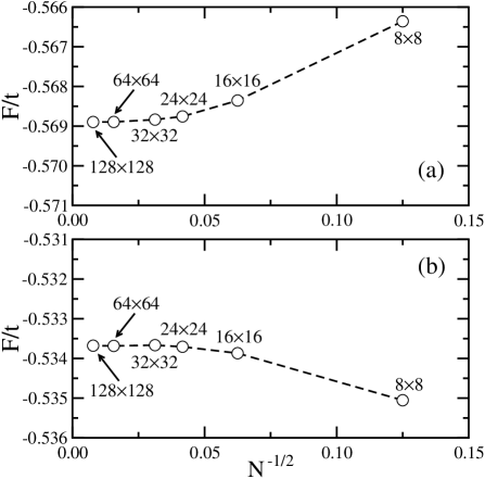
Figure 2: Finite-size scaling of free energy $F$ for: (a) HVS, and (b) HDS, as obtained within the SBA for the Hubbard model at doping $x=1/8$. Parameters: $U=12t$ and $\beta t=1000$.

The above behavior is universal, and a similar tendency appears also in a system with the HDS [see Fig. 2(b)]. Note, however, that in the case of the vertical stripes increasing cluster size lowers the total energy. In contrast, the energy increases when the number of atoms in a cluster with the diagonal stripes gets larger, suggesting that small cluster calculations underestimate (overestimate) the free energy of the vertical (diagonal) stripe phase, respectively, and may thus lead to systematic errors and inconclusive results in some cases. Even though the free energy $F$ saturates quickly with an increasing number of sites in both cases, one should keep the above feature in mind, especially when it comes to investigate the relative stability of vertical and diagonal phases as the inclusion of quantum fluctuations could substantially strengthen this effect. Here we would like to point out another virtue of the present studies performed at temperature $\beta t=1000$. When the temperature is so low, the entropy contribution to the free energy is almost entirely suppressed as $F\simeq\langle H\rangle$, so that one may analyze only the internal energy for different phases, as done below.

III Electron correlation effects in stripe phases

III.1 Physical characterization of stripe phases

Let us now examine the role of strong electron correlations in stabilizing stripe phases of various type. Even though the HFA and SBA yield quantitatively very similar results at half-filling, as recently reviewed by Korbel et al.,Kor03 we show below that they differ markedly in the stripe phases. Indeed, since the HF wave function is a Slater determinant of single particle states, it does not provide enough variational freedom to implement the many-body processes that are relevant for the behavior of interacting fermions. Therefore, one should expect that the inclusion of the correlation effects modifies considerably the distribution of charge and spin density in a stripe phase, especially around nonmagnetic DWs where the correlation corrections are large.Gor99

To illustrate this point, we investigate the charge and magnetization distribution in the SBA and compare them with the reference states obtained in the HFA. To describe the charge distribution, we introduce the local hole density for each inequivalent site $l=(l_{x},l_{y})$ in the stripe unit cell,

$$n_{\rm h}(l_{x})=1-\sum_{\sigma}\bigl{\langle}f^{{\dagger}}_{l\sigma}f_{l\sigma}\bigr{\rangle},$$ (13)

where the average electron density,

$$\langle f^{{\dagger}}_{l\sigma}f_{l\sigma}\rangle=\sum_{\textbf{q}}\Psi_{l\sigma}^{{\dagger}}(\textbf{q})\Psi_{l\sigma}(\textbf{q})n(\epsilon_{\textbf{q}\sigma}),$$ (14)

is given by the real space eigenvectors $\Psi_{l\sigma}(\textbf{q})$ of the effective Hamiltonian (10), and $n(\varepsilon_{\textbf{q}\sigma})$ is the Fermi-Dirac distribution. Further, magnetic domain structures are best described by the modulated magnetization density,

$$S_{\pi}(l_{x})=(-1)^{l_{x}+l_{y}}\frac{1}{2}\sum_{\sigma\sigma^{\prime}}\bigl{\langle}f_{l\sigma}^{{\dagger}}\boldsymbol{\tau}_{\sigma\sigma^{\prime}}f_{l\sigma^{\prime}}\bigr{\rangle},$$ (15)

with a site dependent phase factor $(-1)^{l_{x}+l_{y}}$ compensating the modulation of the staggered magnetization density within a single AF domain, as well as by double occupancy,

$$D(l_{x})=\bigl{\langle}n_{l\uparrow}n_{l\downarrow}\bigr{\rangle}.$$ (16)

III.2 Stripes at low doping $x=1/16$

We begin with the detailed analysis of the charge and magnetization distribution in the stripe phases at low doping $x=1/16$, and compare the results of the SB treatment with those obtained in the HFA. The corresponding SB profiles of the FVS (left) and FDS (right) found in the Hubbard model with $U=6t$ at the doping $x=1/16$ are shown in Fig. 3 (filled circles). In this case nonmagnetic DWs are separated by $d=16$ lattice constants so that the charge (magnetic) unit cell contains sixteen (thirty two) atoms, respectively. In agreement with the calculations of Ref. Sei98, , we note that the hole density $n_{h}$ at nonmagnetic DWs is reduced nearly twice in the SBA as compared to the corresponding HFA value (open circles), regardless of the stripe direction. Moreover, the HF stripe phases are characterized by the enhanced spin polarization of the AF domains. Such a strong modification follows directly from the fact that in the HFA there are only two straightforward possibilities which allow one to diminish the energy of the stripe phase due to the on-site Coulomb repulsion,

$$E_{U}=U\frac{1}{L}\sum_{l_{x}}D(l_{x}).$$ (17)

The simplest way of keeping apart electrons with the opposite spins is by creating strong spin polarization. As a consequence, a well known feature of the HFA is that it overestimates by far the tendency towards symmetry broken states. Another way of reducing $E_{U}$ which may be realized for inhomogeneous charge distribution, for instance in stripe phases, is to suppress locally the total electron density at the sites with small or vanishing magnetization.

In contrast, the SB approach implements local correlations by offering an important mechanism to optimize the on-site interaction by an additional variational parameter, i.e., the boson field $d_{i}$ at each site. In fact, the largest correction of the HF value is obtained at the DW unpolarized sites, where the double occupancy $D$, Eq. (16), shows distinct minima in both phases (see Fig. 3) which allows one to optimize $E_{U}$ even without a great reduction of the actual electron density. Simultaneously, a large value of $D$ within the AF domains suppresses partially the spin polarization of the atoms separating DWs, which enables more intersite excitations and leads to a more favorable kinetic energy gain. Taken together, these two effects are jointly responsible for smoother charge and spin density profiles with respect to the ones found in the HFA. Notice that both approximations yield narrow diagonal stripes, revealing their more localized character as compared to the vertical ones and hence a more favorable average on-site energy, which stabilizes them in the strong coupling regime, as discussed below.

It is quite remarkable that the present calculations performed on large clusters yield also locally stable half-filled stripes both in the HFA and in the SBA without any necessity of quadrupling of the period along the stripes by an additional on-wall spin-density wave.Zaa96 At $x=1/16$, the condition of having one doped hole per two DW atoms requires the charge (magnetic) unit cell containing eight (sixteen) atoms, respectively. The obtained profiles of the HVS (left) and HDS (right) are shown in Fig. 4. Again, one finds a smaller SB charge modulation and a stronger spin polarization of the AF domains in the HFA. Note, however, that contrary to the case with the filled DWs, a narrower charge and spin profile of the vertical stripe with respect to the diagonal one is apparent.

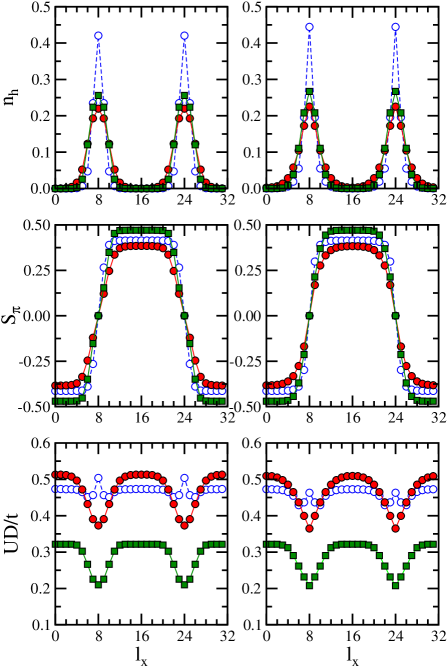
Figure 3: (Color online) Hole and magnetization distribution in filled stripe phases at low doping $x=1/16$: local hole $n_{\rm h}(l_{x})$ density (top), magnetization $S_{\pi}(l_{x})$ density (second row), and double occupancy $D(l_{x})$ (bottom), for the phase with the FVS (left) and FDS (right), found in the Hubbard model on a $128\times 128$ cluster at $\beta t=1000$. Open (filled) circles show the HFA (SBA) results for $U=6t$, respectively, while filled squares denotes the SBA data for $U=12t$.

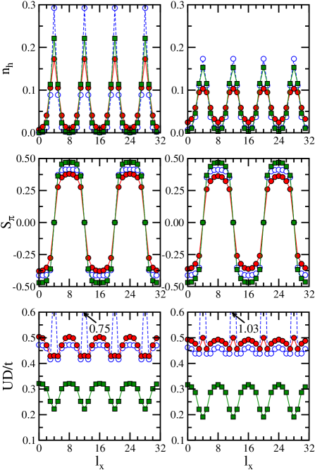
Figure 4: (Color online) The same as in Fig. 3 but for the half-filled stripe phases: HVS (left) and HDS (right). Open (filled) circles show the HF (SB) results for $U=6t$, respectively, while filled squares denotes the SB data for $U=12t$. High values of $UD/t>0.6$ obtained for the DW atoms in the HFA are indicated by arrows.

At strong coupling with $U=12t$ (filled squares), one finds for the most stable phases that the double occupancy profile is interpolating between $D\simeq 4t^{2}/U^{2}$ deep in the magnetic domains (the value expected in an AF phase at half-fillingMol93b ), and the value expected in the PM phase at the actual hole density realized at the domain wall sites, as shown in Table 1. Thus the present approach is flexible enough to implement the compromise between optimized superexchange in the magnetic domains, and optimized (with respect to the local density) double occupancy in the domain walls, with, however, the notable exception of the HDS. In that case this optimization cannot be achieved, and instead one gets a more spread hole distribution. The same tendency is also realized at intermediate coupling.

Table 1: Hole density $n_{\rm h}({\rm DW})$ and double occupancy $D({\rm DW})$ at domain-wall sites, and the corresponding double occupancy in the PM phase $D_{\rm PM}$, as found for various stripe phases in the Hubbard model on an $128\times 128$ cluster at $x=1/16$ doping within the SBA. Parameters: $U=12t$, $\beta t=1000$.

	phase	$n_{\rm h}({\rm DW})$	$D({\rm DW})$	$D_{\rm PM}$
	HDS	0.153	0.016	0.019
	HVS	0.221	0.018	0.018
	FVS	0.256	0.017	0.017
	FDS	0.267	0.017	0.016

Experimentally, two stripe phases have been found: (i) filled diagonal stripe phase, and (ii) half-filled vertical one. Both of them have been observed in LSCO; the former was found around $x=0.02$,Mat00 whereas the latter — at a higher $0.06\leq x\leq 0.125$ doping level.Yam98 In the present calculations these phases were reproduced as two possible ground states of the doped Hubbard model. The crossover found experimentally indicates that the filling and orientation of DWs are indeed closely related in the cuprates. In other words, half-filled stripes tend to be aligned vertically/horizontally, whereas filled ones gain more energy by the diagonal arrangement.

The above important property can also be deduced from the free energies $F$ calculated in the SBA from Eq. (12) for all four stripe phases, given in Table 2. For completeness, the energies of stripe phases are compared with those of the uniform AF phase. Note that the sequence of stripe phases, ordered according to their decreasing energy, is precisely the same in both methods and one does find that the half-filled vertical stripe phase is preferred over its diagonal counterpart, and also that the filled diagonal stripe structure is promoted over the corresponding vertical stripe phase. However, noticeable discrepancies emerge when it comes to compare the on-site Coulomb energy $E_{U}$ and the nearest neighbor kinetic energy determined in SBA,

$$E_{t}=-t\,\frac{1}{L}\sum_{\langle l,l^{\prime}\rangle}\sum_{\sigma\sigma^{\prime}}\bigl{(}z_{l^{\prime}}z^{{\dagger}}_{l}\bigr{)}^{T}_{\sigma^{\prime}\sigma}\bigl{\langle}f^{{\dagger}}_{l\sigma}f_{l^{\prime}\sigma^{\prime}}\bigr{\rangle},$$ (18)

with the ones obtained in the HFA. Most importantly, the inclusion of electron correlations reduces $E_{U}$ of the PM phase by a factor two without a strong suppression of $E_{t}$, which improves significantly its free energy. Therefore, as the average hole density at the half-filled DWs is noticeably smaller than at the filled ones (cf. Figs. 3 and 4), it should also help to stabilize half-filled stripes, because one gains more correlation energy when the nonmagnetic atoms are close to half-filling. These features are clearly seen in Table 2. By comparing the repulsion energy, one finds that $E_{U}$ of both half-filled stripe phases is reduced in the SBA, while $E_{U}$ of the filled ones is even slightly enhanced. As a result, for moderate coupling, the structure with the HVS in the SBA is characterized by the smallest net double occupancy and hence by the most favorable $E_{U}$. Nevertheless, in the SB ground state one recovers the phase with the FDS, as a small energy loss due to the increased on-site energy is easily overcompensated by the kinetic energy gain. The FDS are recovered at strong coupling as well, where the HVS are not even favored by $E_{U}$.

Table 2: Comparison of the site-normalized free energy $F$, on-site Coulomb energy $E_{U}$, and kinetic energy $E_{t}$, as obtained for various phases in the Hubbard model within the HFA (for $U=6t$) and SBA (for $U=6t$ and $12t$) on an $128\times 128$ cluster at doping $x=1/16$ and $\beta t=1000$. For clarity, the phases are listed according to their decreasing energy from top to bottom.

method	$U/t$	phase	$E_{U}/t$	$E_{t}/t$	$F/t$
HFA	6	HDS	0.5185	$-$1.1080	$-$0.5895
		AF	0.4928	$-$1.1198	$-$0.6270
		HVS	0.4892	$-$1.1242	$-$0.6350
		FVS	0.4690	$-$1.1218	$-$0.6528
		FDS	0.4586	$-$1.1154	$-$0.6568
SBA	6	HDS	0.4796	$-$1.1708	$-$0.6912
		AF	0.4943	$-$1.2009	$-$0.7066
		HVS	0.4663	$-$1.1809	$-$0.7146
		FVS	0.4709	$-$1.1929	$-$0.7220
		FDS	0.4671	$-$1.1902	$-$0.7231
SBA	12	AF	0.3181	$-$0.7355	$-$0.4174
		HDS	0.2673	$-$0.7023	$-$0.4350
		HVS	0.2860	$-$0.7356	$-$0.4496
		FVS	0.2930	$-$0.7455	$-$0.4525
		FDS	0.2903	$-$0.7464	$-$0.4561

Finally, it should be emphasized that, in contrast to the HFA, the most favorable SB phase in the moderate coupling regime $U=6t$ for the intersite kinetic energy $E_{t}$ is the AF structure (see Table 2). However, owing to a strong suppression of the double occupancy at nonmagnetic DWs, the existence of stripes opens a possibility for a charge redistribution which optimizes $E_{U}$ even better. Consequently, in the strong coupling regime with $U=12t$ all the stripe phases are favored over the uniform AF order.

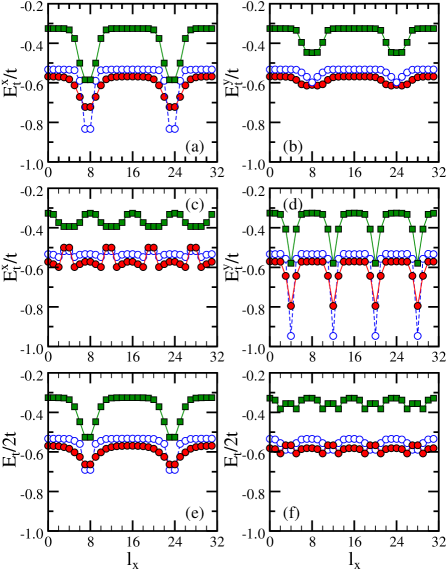
Figure 5: (Color online) Kinetic energy projected on the bonds in the $x$ ($y$) direction, $E_{t}^{x}(l_{x})$ and $E_{t}^{y}(l_{x})$, as found in the phase with either the FVS (a,b) or HVS (c,d), shown in Figs. 3 and 4. Open (filled) circles show the HF (SB) results for $U=6t$, respectively, while filled squares denote the SB data for $U=12t$. Panels (e) and (f) depict the kinetic energy profiles $E_{t}/2t$ of the corresponding FDS and HDS.

In order to identify in detail processes leading to the stripe stabilization, we determined the expectation values of the bond hopping terms, $E_{t}^{x}(l_{x})$ and $E_{t}^{y}(l_{x})$, along the $x$ and $y$ direction, respectively,

$$E_{t}^{x}(l_{x}) =-t\sum_{\sigma\sigma^{\prime}}q_{\sigma\sigma^{\prime}}^{x}(l_{x})\bigl{\langle}f^{{\dagger}}_{(l_{x},l_{y}),\sigma}f_{(l_{x+1},l_{y}),\sigma^{\prime}}\bigr{\rangle},$$ (19)

$$E_{t}^{y}(l_{x}) =-t\sum_{\sigma\sigma^{\prime}}q_{\sigma\sigma^{\prime}}^{y}(l_{x})\bigl{\langle}f^{{\dagger}}_{(l_{x},l_{y}),\sigma}f_{(l_{x},l_{y+1}),\sigma^{\prime}}\bigr{\rangle},$$ (20)

where,

$$q_{\sigma\sigma^{\prime}}^{x}(l_{x}) =\Bigl{(}z_{(l_{x+1},l_{y})}z^{{\dagger}}_{(l_{x},l_{y})}\Bigr{)}^{T}_{\sigma^{\prime}\sigma},$$ (21)

$$q_{\sigma\sigma^{\prime}}^{y}(l_{x}) =\Bigl{(}z_{(l_{x},l_{y+1})}z^{{\dagger}}_{(l_{x},l_{y})}\Bigr{)}^{T}_{\sigma^{\prime}\sigma},$$ (22)

are the corresponding band narrowing factors. The variation of the kinetic energy gain across the unit cell of the phase with the FVS is shown in Figs. 5(a) and 5(b). Deep in the magnetic domains, for large $U$, the kinetic energy in both directions is given by $-4t^{2}/U$, as expected from the large $U$ expansion.Mol93b For the DW sites we obtain that $E_{t}^{y}$ closely reproduces one half of the kinetic energy in the PM phase at the actual hole doping found at these sites. In the two cases shown in Fig. 5, the kinetic energy is weakly influenced by the involved band structure describing the stripe phases, and its profile mostly interpolates between the two expected limits. For the FVS its most significant effect is seen in $E_{t}^{x}$ close to the DW’s, where most of the kinetic energy gain is realized. The same trends are also found for smaller $U$.

As expected, profile of $E_{t}^{x}(l_{x})$ and $E_{t}^{y}(l_{x})$ depends on whether we include local electron correlations or not, as we have already seen that they markedly influence the charge and spin distribution. On the one hand, one sees that the AF domains between stripes are characterized by a more favorable kinetic energy gain in the SBA, owing to a combined effect of a weaker spin polarization and larger doubly occupancies than those found in the HFA. On the other hand, in the SB approach transverse charge fluctuations on the bonds connecting the DWs, with a strong reduction of $D$, and their nearest neighbors, are less efficient than the corresponding ones found in the HFA, where the fact that DWs are nonmagnetic implies much larger $D$ at these sites [cf. Fig. 5(a)]. However, in the SBA, a small $D$ does not necessarily imply a strong reduction of the band narrowing factor. Indeed, the operator $z_{\sigma\sigma^{\prime}}$ describes a sum of the two possible transition channels, either of which may accompany an electron hopping process:Fre92 (singly occupied site) $\rightarrow$ (empty site), or (doubly occupied site) $\rightarrow$ (singly occupied site with a time-reversed spin). Therefore, as the hole density $n_{h}$ at DW sites is large, the first channel should even dominate, which follows from a simple relation,

$$e^{2}=n_{h}+d^{2}.$$ (23)

that follows for a PM site from the local constraint (3). In addition, the HF stripe phase has a twice smaller electron density at the DWs than predicted by the SBA. Altogether, despite large double occupancies at the DWs, the HF kinetic energy gain along the FVS is smaller than the SB one, as shown in Fig. 5(b).

Table 3: Comparison of the site-normalized kinetic energy contribution for bonds along (10) ($E_{t}^{x}$) and (01) ($E_{t}^{y}$) directions, as obtained for the phase with either the FVS or HVS in the Hubbard model on an $128\times 128$ cluster at $x=1/16$ doping and $\beta t=1000$ within the HFA and SBA.

			FVS			HVS
$U/t$	method		$E_{t}^{x}/t$	$E_{t}^{y}/t$		$E_{t}^{x}/t$	$E_{t}^{y}/t$
6	HFA		$-$0.5782	$-$0.5436		$-$0.5337	$-$0.5905
	SBA		$-$0.6085	$-$0.5844		$-$0.5638	$-$0.6171
12	SBA		$-$0.3872	$-$0.3583		$-$0.3562	$-$0.3794

Nevertheless, we have found a confirmation of the trend detected in the earlier calculationsZaa96 ; Nor01 performed in the HFA — also in the SBA the FVS are mainly stabilized not by the charge motion along the DWs but rather by the hole delocalization along the bonds perpendicular to the stripes, i.e., by the so-called solitonic mechanism. This effect is well illustrated by both components, $E_{t}^{x}$ and $E_{t}^{y}$, of the kinetic energy $E_{t}$, shown in Table 3. Here, one observes a significant anisotropy between the HF kinetic energy gain in the $x$ and $y$-directions, $\delta E=E_{t}^{x}-E_{t}^{y}$. This anisotropy is considerably reduced when the local electron correlations are included in the SBA, but remains the driving mechanism stabilizing the stripes.

These results should be now compared with those in Figs. 5(c) and 5(d), obtained for the structure with the HVS. First of all, note that as in the case of the filled stripes, inclusion of the strong electron correlations improves the kinetic energy gain in the AF domains. However, the fact that the half-filled DWs are characterized by a smaller hole density than their filled counterparts results in an entirely different mechanism being responsible for their stability. Indeed, Fig. 5(d) shows that the largest kinetic energy gain is released by the electrons propagating along the half-filled DWs, while the transverse charge fluctuations are less important. This effect is particularly strong in the HFA, where one finds a large anisotropy between $E_{t}^{x}(l_{x})$ and $E_{t}^{y}(l_{x})$ at the DWs. We ascribe this to the fact that the increase of electron density at the nonmagnetic vertical DWs raises double occupancy (cf. Figs. 3 and 4) in this approach, and therefore facilitates the on-wall propagation of the electrons. Moreover, the nearest neighbor sites of the half-filled DW possess a much less quenched $S_{\pi}$, as compared to the neighbors of the filled one. Therefore, all the electrons crossing HVS encounter in this case a stronger on-site potential that develops in the AF domains, which acts to suppress locally $E_{t}^{x}(l_{x})$. A similar amplification (reduction) of the on-wall (transverse) kinetic energy gain, respectively, we have also found in the SBA.

We conclude the above analysis by showing in Table 3 two kinetic energy components $E_{t}^{x}$ and $E_{t}^{y}$ as found for the phase with the HVS. As in the case of the FVS, the presence of the HVS introduces a finite anisotropy between the kinetic energy gain in the $x$ and $y$ directions but while $E_{t}^{x}<E_{t}^{y}$ for the phase with the FVS, the structure with the HVS is characterized instead by $E_{t}^{x}>E_{t}^{y}$.

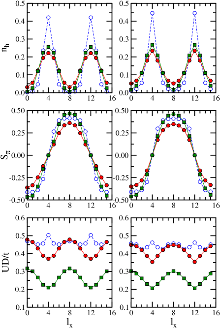
Figure 6: (Color online) Local hole $n_{\rm h}(l_{x})$ (top) and magnetization $S_{\pi}(l_{x})$ (second row) density, as well as double occupancy $D(l_{x})$ (bottom), of the FVS (left) and FDS (right) phase found in the Hubbard model on an $128\times 128$ cluster for doping $x=1/8$ at $\beta t=1000$. Open (filled) circles show the HF (SB) results for $U=6t$, respectively, while filled squares denote the SB data for $U=12t$.

Let us now discuss variation of the kinetic energy gain shown in Figs. 5(e) and 5(f) across the unit cell of the phase with either the FDS or HDS. Here one finds that due to the symmetry $E_{t}/2=E_{t}^{x}=E_{t}^{y}$. Therefore, based on Fig. 5(e) showing substantial kinetic energy gain due to transverse hopping processes onto and off the stripe, one might expect that such a structure enables the largest kinetic energy gain among the stripe phases. In fact, it happens only in the strong coupling regime with $U=12t$, as reported in Table 2. In contrast, a weak charge modulation induced by the HDS results in a smooth kinetic energy profile without a particularly severe gain in the vicinity of the DWs. As a consequence, this phase is characterized by the smallest kinetic energy gain regardless of both the approach and the strength of $U$ (see Table 2).

III.3 Stripes at intermediate doping $x=1/8$

We turn now to a short discussion of the stripe profiles shown in Figs. 6 and 7, obtained at a twice higher doping level $x=1/8$. The stripe structures at this doping confirm the main conclusions of the previous Section concerning the stripe stability. One finds again that the transverse (parallel) hopping stabilizes the structures with filled (half-filled) vertical DWs, respectively (cf. Fig. 8). In addition, we point out the most prominent changes with respect to the low doping regime.

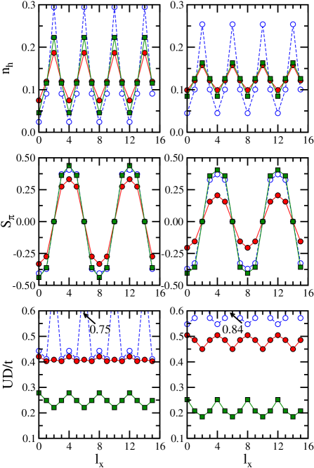
Figure 7: (Color online) The hole density $n_{\rm h}(l_{x})$ (top), magnetization density $S_{\pi}(l_{x})$ (second row), and double occupancy $D(l_{x})$ (bottom) for the half-filled stripe phases: HVS (left) and HDS (right). Open (filled) circles show the HF (SB) results for $U=6t$, respectively, while filled squares denote the SB data for $U=12t$. Doping, cluster size and temperature as in Fig. 6.

First of all, the increased doping acts to shrink the distance between the filled DWs according to the formula $d=1/x$, so that the charge (magnetic) unit cell is reduced and involves now eight (sixteen) atoms, respectively, as depicted in Fig. 6. One finds that the charge distribution is smoother in the SBA than in the HFA, and in the moderate coupling regime $U=6t$ the highest hole density on the nonmagnetic ($S_{\pi}=0$) DW atoms is only $n_{h}\simeq 0.22\div 0.24$. This demonstrates that the filled stripe phases are truly itinerant systems with modulated charge density.

Table 4: The same as in Table 2 but for $x=1/8$.

method	$U/t$	phase	$E_{U}/t$	$E_{t}/t$	$F/t$
HFA	6	HDS	0.6321	$-$1.2330	$-$0.6009
		AF	0.5148	$-$1.1808	$-$0.6660
		HVS	0.5031	$-$1.1800	$-$0.6769
		FVS	0.4649	$-$1.1777	$-$0.7128
		FDS	0.4432	$-$1.1639	$-$0.7207
SBA	6	HDS	0.4815	$-$1.2713	$-$0.7898
		AF	0.4563	$-$1.2563	$-$0.8000
		HVS	0.4083	$-$1.2098	$-$0.8014
		FVS	0.4269	$-$1.2470	$-$0.8201
		FDS	0.4123	$-$1.2324	$-$0.8201
SBA	12	HDS	0.2130	$-$0.7467	$-$0.5337
		AF	0.2726	$-$0.8112	$-$0.5386
		HVS	0.2486	$-$0.8175	$-$0.5689
		FVS	0.2645	$-$0.8396	$-$0.5751
		FDS	0.2588	$-$0.8409	$-$0.5821

However, the experimentally established distance between stripes in Nd-LSCO at $x=1/8$ doping is equal to $d=4$,Tra95Nd implying that de facto less holes are doped per one DW site, and consequently DWs are only partly filled by holes. Indeed, other local minima are obtained in the SB calculations for the charge (magnetic) unit cells of the half-filled stripe phases, containing four (eight) atoms, respectively, as shown in Fig. 7. Also these phases are itinerant, with the SB hole densities at $U=6t$ less than 0.2 at the DW sites for both half-filled stripe phases. Moreover, correlations implemented in the SB approach guarantee that electrons avoid each other and the double occupancy is the lowest $D\simeq 0.07$ at the half-filled vertical DW sites, while in the HFA one finds instead a large value $D_{0}\simeq 0.13$. However, it is remarkable that the SB double occupancy $D$ is practically site independent in the phase with the HVS, in spite of rather different electron densities at the DW sites and within the AF domains.

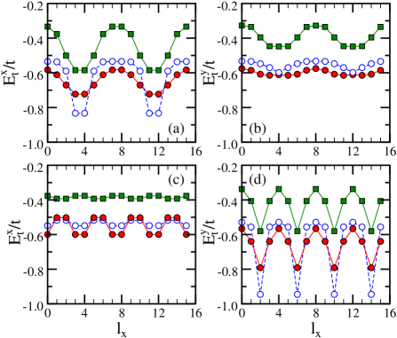
Figure 8: (Color online) Kinetic energy $E_{t}^{x}(l_{x})$ and $E_{t}^{y}(l_{x})$ projected on the bonds along the $x$ and $y$ direction, as obtained for the phase with either the FVS (a,b), or HVS (c,d), shown in Figs. 6 and 7, respectively. Open (filled) circles show the HF (SB) results for $U=6t$, respectively, while filled squares denotes the SB data for $U=12t$.

Next, we address a generic crossover found in the SBA from the FDS to their vertical counterparts taking place upon doping. We have seen from the respective charge distributions in Fig. 6 that a certain amount of holes proliferates out of the DWs, reducing double occupancies in the AF domains. Consequently, the on-site energy gains become less important, which explains the transition towards the phase with the FVS, being a more favorable structure for the charge dynamics. In fact, for $U=6t$, this crossover occurs precisely at $x=1/8$, so that both phases become degenerate, as reported in Table 4, while in the strong coupling regime $U=12t$ one recovers in the ground state the phase with the FDS. Moreover, as the doped holes are now only weakly localized at the DW sites, a nonuniform charge distribution in the AF domains amplifies the anisotropy between the kinetic energy gain $E_{t}^{x}$ and $E_{t}^{y}$ (cf. Table 5).

Table 5: The same as in Table 3 but for $x=1/8$.

			FVS			HVS
$U/t$	method		$E_{t}^{x}/t$	$E_{t}^{y}/t$		$E_{t}^{x}/t$	$E_{t}^{y}/t$
6	HFA		$-$0.6234	$-$0.5543		$-$0.5331	$-$0.6469
	SBA		$-$0.6468	$-$0.6002		$-$0.5504	$-$0.6593
12	SBA		$-$0.4486	$-$0.3910		$-$0.3848	$-$0.4327

III.4 Electronic structure of stripe phases

Let us analyze in more detail the electronic structure obtained for the stripe phases in the low doping regime. Since the stripe phases consist of a superposition of magnetic domains with a 2D character, and domain walls of 1D character, it is worth determining to which part of the spectrum each of them contribute, and to which extend they mix. The DOS of a pure 2D AF phase exhibits a gap ($\Delta\sim U$) separating two van Hove singularities lying at the top (bottom) of the lower (upper) Hubbard subbands, here representing the dynamical Hubbard bands. In 1D case the van Hove singularities are located at the lower and upper band edges.

Let us consider the actual DOS for the phase with the HVS in the moderate coupling regime $U=6t$ — it consists indeed of two Hubbard subbands at low and high energies, lower Hubbard band (LHB) and upper Hubbard band (UHB), separated by a gap of $\sim 5t$ in the HFA and $\sim 2.6t$ in the SBA, see Figs. 9(a) and 9(b). So strong reduction of the gap with a similar value of the magnetization in the AF domains is the first correlation effect identified in the electronic structure.

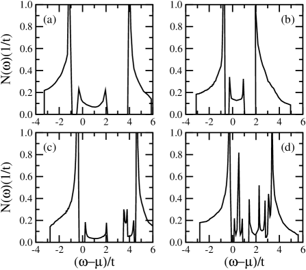
Figure 9: Density of states $N(\omega)$ of the phase with: (a,b) HVS, shown in the left panels of Fig. 4; (c,d) FVS, depicted in the left panels of Fig. 3, as obtained within the HFA (left) and the SBA (right) in the moderate coupling regime $U=6t$ for doping $x=1/16$.

Furthermore, the formation of stripes with nonmagnetic sites results in additional electronic states within the Mott-Hubbard gap. These new structures contain parts of the spectral density below the Fermi energy, both in the HFA and in the SBA, indicating that half-filled stripe phases are metallic. Note also that the nonmagnetic stripes hybridize only weakly with the neighboring AF domains, since they are mainly stabilized by the electrons propagating along them, so this part of $N(\omega)$ is reminiscent of the tight binding DOS for a linear chain with nearest neighbor hopping, and has the characteristic peaks at the edges. We recall that in 1D case the van Hove singularities are located at the lower and upper band edges, as found here for the in-gap bands. Similar to the Hubbard subbands, also the partly filled electronic subbands in the gap are substantially narrowed by the correlation effects in the SBA.

In the case of filled vertical stripe phases shown in Figs. 9(c) and 9(d), the states in the gap are empty. This was actually pointed out rather early as the microscopic reason responsible for the stability of such phases in the HFA. Zaa96 The most prominent feature of the DOS for FVS phase is again a striking similarity of the mid-gap part of $N(\omega)$ to the DOS of a linear chain. The width is somewhat reduced indicating a more localized character of these states. In contrast with the phase with the HVS, a stronger hybridization with the AF domains influences the UHB so that a certain amount of its states is shifted towards a lower energy and forms a separate segment of $N(\omega)$ [cf. Fig. 9(c)].

Finally, in Fig. 9(d) we show the DOS of the phase with the FVS which follows from the SBA. In this case the charge and spin density profiles are more spread out and a weaker anisotropy between the tranverse and parallel electron motion, as compared to the HF ones, results in a less clear character of the mid-gap part of $N(\omega)$, with a large peak in the middle being now a characteristic feature of the 2D tight binding DOS. Notice also an insulating nature of both filled stripes. Indeed, as the mid-gap states are now entirely empty, the Fermi energy lies inside the gap between the highest occupied state of the LHB and the bottom of the mid-gap band.

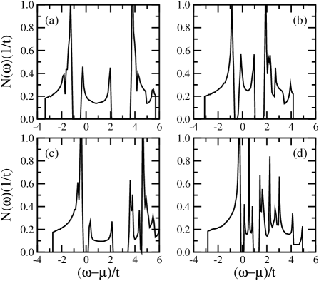
Figure 10: Density of states $N(\omega)$ of the phase with: (a,b) HVS, shown in the left panels of Fig. 7; (c,d) FVS, depicted in the left panels of Fig. 6, as obtained within the HFA (left) and SBA (right) in the moderate coupling regime $U=6t$ for doping $x=1/8$.

For the higher doping $x=1/8$ one finds similar features in the DOS of both HVS and FVS phases. The spectral intensity is here redistributed, showing a systematic transfer of the spectral weight from the UHB into these states and the LHB upon doping, in agreement with a strong coupling perturbation theory for the Hubbard model.Esk94 In addition, the spectral weight is also transfered into the mid-gap part of $N(\omega)$, which grows with an increasing number of stripes in the cluster.

IV Stripe phases in the extended hopping model

IV.1 Crossover to vertical stripe phases

Thus far we have worked out that in the strongly correlated regime relevant for the cuprates a structure with the FDS (HVS) is the lowest in energy among the stripe structures with the filled (half-filled) DWs, respectively. Therefore, an interesting question occurs — which microscopic parameters decide whether the phase with the FDS or the one with the HVS is more stable. To clarify this point we have investigated in the SBA the competition between the stripe phases in the $t$-$t^{\prime}$-$U$ model with $U=12t$. The chosen value of the Coulomb interaction gives the ratio $J/t=1/3$ which corresponds to the physical value in the cuprates.Jef92

Fig. 11(a) shows the effect of increasing next-nearest neighbor hopping $|t^{\prime}|$ on the free energy $F$ of all four stripe phases, as well as of the uniform AF phase at the hole doping $x=1/16$ and $U=12t$. Here, the most striking result is that while increasing $|t^{\prime}|$ only weakly influences the energy of the AF phase, it modifies substantially $F$ of the stripe phases. Moreover, it clearly stabilizes half-filled stripes reducing simultaneously stability of the filled DWs. To appreciate better the enhanced stability of the half-filled stripes with respect to the latter ones, we analyze the average kinetic energy $E_{t^{\prime}}$ per diagonal bond as a function of increasing $|t^{\prime}|$, obtained in the AF and PM phases for a few doping levels: $x=1/16$ (dot-dashed line), $x=1/8$ (dashed line), and $x=1/5$ (solid line) (see Fig. 12). One finds that a negative next-nearest neighbor hopping ($t^{\prime}/t<0$) yields first a positive kinetic energy contribution with the loss being proportional to doping. On the one hand, hopping processes associated with $t^{\prime}$ are partly suppressed in the AF phase by both the reduction of double occupancies and the increase of spin polarization. On the other hand, in the PM phase, these processes might be optimized only by the first effect, which results in a much more severe loss of the energy. However, these trends also involve a reduction of the nearest neighbor hopping processes and therefore they cannot be maintained above a certain critical value of $t^{\prime}$. As a result, $E_{t^{\prime}}$ changes its sign and becomes negative (cf. Fig. 12).

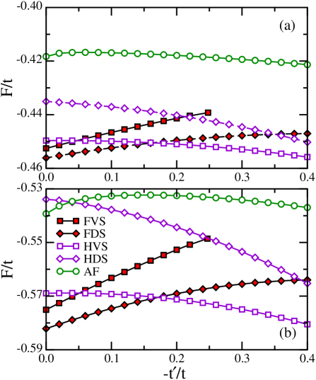
Figure 11: (Color online) Site-normalized SB free energy $F$ of the phase with the FVS, FDS, HVS, and HDS, as well as of the AF phase, as a function of increasing next-nearest neighbor hopping $|t^{\prime}|$ for $U=12t$ in the: (a) underdoped regime $x=1/16$; (b) moderately doped regime $x=1/8$.

Turning back to the analysis of the stripe stability, the fact that the energy loss due to the $t^{\prime}$ term follows predominately from the hopping processes at the nonmagnetic DWs explains immediately why a finite $t^{\prime}$ promotes partially filled stripes. Indeed, as the average hole density at the half-filled DWs is smaller than at the filled ones (cf. Figs. 3 and 4), one should lose less kinetic energy in the former case, especially in the phase with the HDS, where the reduction of the hole density at the DWs is the strongest. Consequently, as depicted in Fig. 11(a), this phase is characterized by the largest free energy gain upon increasing $|t^{\prime}|$. Further, increasing $|t^{\prime}|$ strongly interferes with the solitonic mechanismZaa96 stabilizing the FVS by the transverse hopping and hence such a structure becomes unstable at $t^{\prime}/t\simeq-0.248$. In contrast, narrower FDS are stabilized to a lesser degree by this mechanism remaining a stable solution in the entire region $0<|t^{\prime}/t|<0.4$. Finally, the energy difference between the phase with the HVS and the one with the FDS gradually diminishes so that the former becomes the ground state of the system at $t^{\prime}/t\simeq-0.16$.

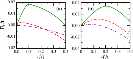
Figure 12: (Color online) Average kinetic energy $E_{t^{\prime}}$ per diagonal bond as a function of increasing next-nearest neighbor hopping $|t^{\prime}|$ for: (a) AF phase, and (b) PM phase, as obtained for $U=12t$. Dot-dashed, dashed, and solid line shows the results for $x=1/16$, $x=1/8$, and $x=1/5$ doping, respectively.

In order to get a more quantitative insight into the mechanism of the crossover between the above phases, we show in Table 6 decomposition of their free energy into the on-site Coulomb energy $E_{U}$ as well as into both kinetic energy contributions $E_{t}$ and $E_{t^{\prime}}$. On the one hand, the robust stability of the FDS in the absence of $t^{\prime}$, follows mainly from a large kinetic energy gain $E_{t}$ (cf. Table 2). In contrast, at the expense of $E_{t}$, the structure with the HVS better optimizes the double occupancy energy $E_{U}$, being however less stable than the one with the FDS. On the other hand, as we have already found, a negative next-nearest neighbor hopping tends to yield a positive kinetic energy contribution, but the actual sign depends both on the value of $t^{\prime}$ and on the filling of the DWs. Indeed, the presence of the half-filled stripes clearly helps to alterate the disadvantageous sign of $E_{t^{\prime}}$ so that it is negative already for $t^{\prime}=-0.3t$ (cf. Table 6). Conversely, in the phase with the FDS, in spite of a stronger reduction of double occupancies with a concomitant detriment of $E_{t}$, delocalization of electrons due to a finite $t^{\prime}=-0.3t$ still costs a small amount of energy. All these features act to stabilize the HVS in the ground state.

Table 6: Free energy $F$ per site, on-site Coulomb energy $E_{U}$ as well as kinetic energy $E_{t}$ and $E_{t}^{\prime}$ contributions, as obtained for the phase with either the HVS or FDS in the extended Hubbard model from the SBA on an $128\times 128$ cluster. Parameters: $U=12t$, $t^{\prime}=-0.3t$ and $\beta t=1000$.

$x$	phase	$E_{U}/t$	$E_{t}/t$	$E_{t^{\prime}}/t$	$F/t$
$1/16$	FDS	0.2775	$-$0.7292	0.0039	$-$0.4478
	HVS	0.2767	$-$0.7225	$-$0.0071	$-$0.4529
$1/8$	FDS	0.2332	$-$0.8064	0.0077	$-$0.5655
	HVS	0.2300	$-$0.7911	$-$0.0138	$-$0.5749

Based on the above discussion one could expect that at a higher doping, the HVS would take over the FDS for a much smaller value of $|t^{\prime}|$. Indeed, as shown in Table 6, $x=1/8$ provides a more significant energy lowering of the phase with the HVS due to a twice larger $E_{t^{\prime}}$ gain. Simultaneously, the energy loss in the structure with the FDS due to the $t^{\prime}$ processes is twice as large as for $x=1/16$. Consequently, increasing $|t^{\prime}|$ destabilizes now easier the FVS and one finally loses this solution already at $t^{\prime}/t\simeq-0.247$, as illustrated in Fig. 11(b). Nevertheless, one reads off from Fig. 11(b) that a change of the ground state upon increasing $|t^{\prime}|$ takes place in this case at even slightly larger value $|t^{\prime}|\simeq 0.17t$. The explanation is contained in Table 6: a higher doping diminishes the double occupancies and additionally it is reflected in a higher mobility of the electrons. As a consequence, the relative energy

$$\delta F=F_{\rm FDS}-F_{\rm HVS},$$ (24)

varies, in the absence of $t^{\prime}$, from $\delta F=-0.0065t$ for $x=1/16$ to $\delta F=-0.0132t$ at $x=1/8$, which demonstrates an increasing stability of the FDS. Therefore, the condition of having the crossover at $x=1/8$ requires overcompensation of the larger $|\delta F|$ and thus the transition is now slightly moved towards the larger $|t^{\prime}|$.

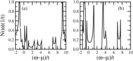
Figure 13: Density of states $N(\omega)$ of the ground state with: (a) FDS for $x=1/16$ and $t^{\prime}=0$; (b) HVS for $x=1/8$ and $t^{\prime}=-0.3t$, as obtained for large Coulomb interaction $U=12t$.

Altogether, Fig. 11 enables scenario in which doping-induced increase in the amplitude of $t^{\prime}$ results in a drastic change in the spin modulation from the diagonal to vertical/horizontal one, as observed experimentally in LSCO at $x\simeq 0.06$. The conjecture that $|t^{\prime}|$ is suppressed in underdoped regime and grows with increasing $x$, seems to be also supported by the recent ED studies showing that $t^{\prime}$ helps to stabilize the superconductivity in the optimally and overdoped regime but it is harmful in the underdoped regime.Shi04 Moreover, inelastic neutron scattering experiments on YBCO, a bilayered compound with a larger than LSCO next-nearest neighbor hopping term $|t^{\prime}|\simeq 0.3t$,Pav01 have established the presence of the IC vertical/horizontal spin fluctuations throughout its entire superconducting regime,Dai01 implying that such a modulation is: (i) realized easier for larger $|t^{\prime}|$, and (ii) more advantageous for the superconductivity than the diagonal one. Note, however, that it remain puzzling why the average filling of diagonal DWs changes from one to $(1/\sqrt{2})$ hole per one DW site in the very low doping regime $x\sim 0.03$. Unfortunately, we could not address this issue here as it requires calculations for still larger unit cells which could not be performed at present.

IV.2 Changes in the electronic structure due to finite $t^{\prime}$

Remarkably, in the present approach, the two possible ground states have entirely different physical properties being either insulating or metallic. Indeed, the DOS of the ground state with the FDS obtained in the Hubbard model with $t^{\prime}=0$ at $x=1/16$ consists of clearly seen two distinct maxima corresponding to the Hubbard bands, while the Fermi energy falls within a gap which results from the magnetic order [cf. Fig. 13(a)]. Interestingly, due to a strong Coulomb repulsion $U=12t$ and consequently small band narrowing factors, instead of the ones as for $U=6t$, one finds here four separated midgap bands. In contrast, as shown in Fig. 13(b), the Fermi energy crosses the midgap states of the structure with the HVS, which is the ground state of the Hamiltonian with $x=1/8$ and $t^{\prime}=-0.3t$, enabling charge transport in agreement with the data for LSCO.

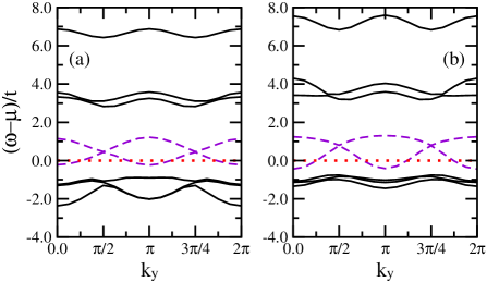
Figure 14: (Color online) Electronic structure of the phase with the HVS as a function of parallel momentum $k_{y}$, calculated from the unit cell shown in Fig. 1(a) on an 8$\times$8 cluster within the SB method for $U/t=12$, and: (a) $t^{\prime}=0$, (b) $t^{\prime}/t=-0.3$. Solid (dashed) lines correspond to the bulk (mid-gap) bands, respectively, whereas the dotted lines indicate the Fermi level.

We also note that, in agreement with Ref. Sei04, , a negative $t^{\prime}$ leads to a distinct broadening of the partially filled mid-gap band induced by the HVS and consequently it shifts these states to a lower energy, as depicted in Fig. 14. Conversely, the energy gain due to such a modification of the electronic structure is not possible in the case of the FDS as their mid-gap states are entirely unoccupied. Thus, the puzzling role of $t^{\prime}$ in promoting the half-filled DWs is clarified.

V Discussion and Summary

We have developed a simple but powerful SB approach which allows one to investigate various stripe phases with a large unit cell and carry out the calculations on a large ($128\times 128$) cluster. Having presented the theoretical framework in Sec. II, we have shown in Sec. II.4 that our method provides a unique opportunity to obtain unbiased results at low temperature $\beta t=1000$, as well as to eliminate the role of finite size effects. The electron correlation effects beyond the HF were implemented within the SB method. Therefore, the stripe phases found in the present approach are stabilized not due to particular boundary conditions, but they represent a generic instability of the strongly correlated electron system doped by holes.

Then, in Sec. III we have analyzed the stability of the idealized filled as well as the half-filled stripes in the Hubbard model at two representative doping levels $x=1/16$ and $x=1/8$. However, the true ground state could correspond to neither filled nor half-filled stripes, as the optimal filling might vary with doping. By comparing the SB charge and spin density profiles with the ones obtained in the HFA in moderate coupling regime with $U=6t$, we have emphasized the role of a proper treatment of electron correlations. In particular, we have found that the largest correction of the HF value is obtained at the DW unpolarized sites, where the double occupancy $D$ shows distinct minima, which allows one to optimize the on-site Coulomb energy $E_{U}$ even without a great reduction of the actual electron density. Simultaneously, an enhanced value of $D$ in SB approach suppresses partially the spin polarization of the atoms within the AF domains, which enables more intersite excitations and leads to a more favorable kinetic energy gain. Taken together, these two effects are responsible for smoother SB charge and spin density profiles with respect to the ones found in the HFA. Moreover, we have shown that at strong coupling with $U=12t$ the SB double occupancy profile is interpolating between $4t^{2}/U^{2}$ deep in the magnetic domains and the value expected in the PM phase at the hole density obtained at the DW sites.

However, the most prominent result of our extensive studies of the kinetic energy was a demonstration of a close relationship between the filling and the direction of the largest kinetic energy gain. Indeed, we have shown that while deep within the magnetic domains the kinetic energy in both directions is given by $-4t^{2}/U$, as expected from large $U$ expansions,Mol93b in the neighborhood of DWs the physical situation is much more complex and depends on the microscopic properties of the considered stripe phase. Especially, it turns out that the HVS are predominately stabilized by the electrons propagating along them, whereas their filled counterparts might be considered as a set of weakly coupled solitons as their stability follows to a large extent from the transverse hopping across them.

Finally, proceeding from the experimental motivation, based on the doping-induced change of the spatial orientation of the DWs in the cuprates, we have investigated the effect of the effective next-nearest neighbor hopping $t^{\prime}$ on the stripe stability. Remarkably, we have found that a subtle increase of the amplitude of $t^{\prime}$ with increasing doping could explain the observed transition from the filled insulating diagonal stripes towards the half-filled metallic vertical/horizontal ones in the cuprates. As the effective hopping $t^{\prime}$ is different for hole-doped and electron-doped cuprates,Fei96 and the doped holes delocalize the magnetic moments at Cu sites, it might be expected that $|t^{\prime}|$ increases with doping. This poses an interesting physical problem for the parameters of the effective one-band model for the cuprates which should be resolved by future studies. Such a doping dependent $t^{\prime}$ may also result from the change of lattice parameters upon doping observed in most superconducting cuprates.Ngu81

- (1) S. A. Kivelson, I. P. Bindloss, E. Fradkin, V. Oganesyan, J. M. Tranquada, A. Kapitulnik, and C. Howald, Rev. Mod. Phys. 75, 1201 (2003).
- (2) P. A. Lee, N. Nagaosa, and X.-G. Wen, Rev. Mod. Phys. 78, 17 (2006).
- (3) S. M. Hayden, H. A. Mook, P. Dai, T. G. Perring, and F. Doǧan, Nature 429, 531 (2004); C. Stock, W. J. L. Buyers, R. A. Cowley, P. S. Clegg, R. Coldea, C. D. Frost, R. Liang, D. Peets, D. Bonn, W. N. Hardy, and R. J. Birgeneau, Phys. Rev. B71, 024522 (2005); V. Hinkov, P. Bourges, S. Pailhes, Y. Sidis, A. Ivanov, C. T. Lin, D. P. Chen, and B. Keimer, arXiv:cond-mat/0601048.
- (4) N. B. Christensen, D. F. McMorrow, H. M. Rønnow, B. Lake, S. M. Hayden, G. Aeppli, T. G. Perring, M. Mangkorntong, M. Nohara, and H. Takagi, Phys. Rev. Lett. 93, 147002 (2004).
- (5) J. M. Tranquada, H. Woo, T. G. Perring, H. Goka, G. D. Gu, G. Xu, M. Fujita and K. Yamada, Nature 429, 534 (2004).
- (6) G. Seibold and J. Lorenzana, Phys. Rev. Lett. 94, 107006 (2005); M. Vojta, T. Vojta, and R. K. Kaul, arXiv:cond-mat/0510448 (unpublished).
- (7) J. M. Tranquada, B. J. Sternlieb, J. D. Axe, Y. Nakamura, and S. Uchida, Nature 375, 561 (1995).
- (8) J. Zaanen and O. Gunnarsson, Phys. Rev. B40, 7391 (1989); D. Poilblanc and T. M. Rice, ibid. 39, 9749 (1989); H. J. Schulz, J. Phys. (Paris) 50, 2833 (1989); Phys. Rev. Lett. 64, 1445 (1990); K. Machida, Physica C 158, 192 (1989); M. Inui and P. B. Littlewood, Phys. Rev. B44, 4415 (1991).
- (9) M. Fujita, H. Goka, K. Yamada, J. M. Tranquada, and L. P. Regnault, Phys. Rev. B70, 104517 (2004).
- (10) P. Abbamonte, A. Rusydi, S. Smadici, G. D. Gu, G. A. Sawatzky, and D. L. Feng, Nature Physics 1, 155 (2005).
- (11) A. R. Moodenbaugh, Y. Xu, M. Suenaga, T. J. Folkerts, and R. N. Shelton, Phys. Rev. B38, 4596 (1988); M. K. Crawford, R. L. Harlow, E. M. McCarron, W. E. Farneth, J. D. Axe, H. Chou, and Q. Huang, ibid. 44, 7749 (1991).
- (12) K. Yamada, C. H. Lee, K. Kurahashi, J. Wada, S. Wakimoto, S. Ueki, H. Kimura, Y. Endoh, S. Hosoya, G. Shirane, R. J. Birgeneau, M. Greven, M. A. Kastner, and Y. J. Kim, Phys. Rev. B57, 6165 (1998).
- (13) J. M. Tranquada, J. D. Axe, N. Ichikawa, A. R. Moodenbaugh, Y. Nakamura, and S. Uchida, Phys. Rev. Lett. 78, 338 (1997).
- (14) P. Dai, H. A. Mook, R. D. Hunt, and F. Doǧan, Phys. Rev. B63, 054525 (2001).
- (15) H. A. Mook, P. Dai, and F. Doǧan, Phys. Rev. Lett. 88, 097004 (2002).
- (16) S. Wakimoto, G. Shirane, Y. Endoh, K. Hirota, S. Ueki, K. Yamada, R. J. Birgeneau, M. A. Kastner, Y. S. Lee, P. M. Gehring, and H. S. Lee, Phys. Rev. B60, 769 (1999); S. Wakimoto, R. J. Birgeneau, M. A. Kastner, Y. S. Lee, R. Erwin, P. M. Gehring, S. H. Lee, M. Fujita, K. Yamada, Y. Endoh, K. Hirota, and G. Shirane, ibid. 61, 3699 (2000); M. Fujita, K. Yamada, H. Hiraka, P. M. Gehring, S. H. Lee, S. Wakimoto, and G. Shirane, ibid. 65, 064505 (2002).
- (17) S. Wakimoto, J. M. Tranquada, T. Ono, K. M. Kojima, S. Uchida, S.-H. Lee, P. M. Gehring, and R. J. Birgeneau, Phys. Rev. B64, 174505 (2001).
- (18) M. Matsuda, Y. S. Lee, M. Greven, M. A. Kastner, R. J. Birgeneau, K. Yamada, Y. Endoh, P. Böni, S.-H. Lee, S. Wakimoto, and G. Shirane, Phys. Rev. B61, 4326 (2000); M. Matsuda, M. Fujita, K. Yamada, R. J. Birgeneau, M. A. Kastner, H. Hiraka, Y. Endoh, S. Wakimoto, and G. Shirane, ibid. 62, 9148 (2000); M. Matsuda, M. Fujita, K. Yamada, R. J. Birgeneau, Y. Endoh, and G. Shirane, ibid. 65, 134515 (2002).
- (19) V. Sachan, D. J. Buttrey, J. M. Tranquada, J. E. Lorenzo, and G. Shirane, Phys. Rev. B51, 12742 (1995); J. M. Tranquada, D. J. Buttrey, and V. Sachan, ibid. 54, 12318 (1996); R. Kajimoto, K. Ishizaka, H. Yoshizawa, and Y. Tokura, ibid. 67, 014511 (2003).
- (20) S. R. White and D. J. Scalapino, Phys. Rev. Lett. 80, 1272 (1998); Phys. Rev. B60, 753 (1999).
- (21) D. Góra, K. Rościszewski, and A. M. Oleś, Phys. Rev. B60, 7429 (1999).
- (22) T. Tohyama, S. Nagai, Y. Shibata, and S. Maekawa, Phys. Rev. Lett. 82, 4910 (1999).
- (23) P. Wróbel and R. Eder, Phys. Rev. B62, 4048 (2000); P. Wróbel, A. Macia̧g, and R. Eder, J. Phys.: Condens. Matter 18, 1249 (2006); arXiv:cond-mat/0408703 (unpublished).
- (24) A. L. Chernyshev, A. H. Castro Neto, and A. R. Bishop, Phys. Rev. Lett. 84, 4922 (2000); A. L. Chernyshev, S. R. White, and A. H. Castro Neto, Phys. Rev. B65, 214527 (2002).
- (25) M. Fleck, A. I. Lichtenstein, E. Pavarini, and A. M. Oleś, Phys. Rev. Lett. 84, 4962 (2000); M. Fleck, A. I. Lichtenstein, and A. M. Oleś, Phys. Rev. B64, 134528 (2001).
- (26) M. G. Zacher, R. Eder, E. Arrigoni, and W. Hanke, Phys. Rev. Lett. 85, 2585 (2000); Phys. Rev. B65, 045109 (2002).
- (27) F. Becca, L. Capriotti, and S. Sorella, Phys. Rev. Lett. 87, 167005 (2001); J. Riera, Phys. Rev. B64, 104520 (2001).
- (28) A. M. Oleś and J. Zaanen, Phys. Rev. B39, 9175 (1989).
- (29) G. Kotliar and A. E. Ruckenstein, Phys. Rev. Lett. 57, 1362 (1986).
- (30) R. Frésard and P. Wölfle, J. Phys.: Condens. Matter 4, 3625 (1992).
- (31) R. Frésard and W. Zimmermann, Phys. Rev. B58, 15288 (1998); I. Yang, E. Lange, and G. Kotliar, ibid. 61, 2521 (2000).
- (32) B. Möller and P. Wölfle, Phys. Rev. B48, 10320 (1993); R. Doradziński and J. Spałek, ibid. 56, 14239 (1997); 58, 3293 (1998).
- (33) R. Frésard and G. Kotliar, Phys. Rev. B56, 12909 (1997); H. Hasegawa, ibid. 56, 1196 (1997); A. Klejnberg and J. Spałek, ibid. 57, 12041 (1998); 61, 15542 (2000); R. Frésard and M. Lamboley, J. Low Temp. Phys. 126, 1091 (2002); L. F. Feiner and A. M. Oleś, Phys. Rev. B71, 144422 (2005).
- (34) G. Seibold, E. Sigmund, and V. Hizhnyakov, Phys. Rev. B57, 6937 (1998).
- (35) G. Seibold, C. Castellani, C. Di Castro, and M. Grilli, Phys. Rev. B58, 13506 (1998).
- (36) A. Damascelli, Z. Hussain, and Z.-X. Shen, Rev. Mod. Phys. 75, 473 (2003).
- (37) T. Tohyama, Phys. Rev. B70, 174517 (2004).
- (38) L. F. Feiner, J. H. Jefferson, and R. Raimondi, Phys. Rev. Lett. 76, 4939 (1996); E. Pavarini, I. Dasgupta, T. Saha-Dasgupta, O. Jepsen, and O. K. Andersen, ibid. 87, 047003 (2001).
- (39) P. Prelovšek and A. Ramšak, Phys. Rev. B72, 012510 (2005).
- (40) C. T. Shih, T. K. Lee, R. Eder, C.-Y. Mou, and Y. C. Chen, Phys. Rev. Lett. 92, 227002 (2004).
- (41) G. Seibold and J. Lorenzana, Phys. Rev. B69, 134513 (2004).
- (42) M. Raczkowski, A. M. Oleś, and R. Frésard, Phys. Status Solidi B 243, 128 (2006).
- (43) A. H. Castro Neto, Phys. Rev. B64, 104509 (2001).
- (44) J. Zaanen and A. M. Oleś, Ann. Phys. (Leipzig) 5, 224 (1996).
- (45) R. Frésard and T. Kopp, Nucl. Phys. B 594, 769 (2001).
- (46) R. Frésard and P. Wölfle, Int. J. Mod. Phys. B 6, 685 (1992); ibid. 3087(E) (1992).
- (47) W. Zimmermann, R. Frésard, and P. Wölfle, Phys. Rev. B56, 10097 (1997).
- (48) S. Florens, A. Georges, G. Kotliar, and O. Parcollet, Phys. Rev. B66, 205102 (2002).
- (49) R. Frésard, M. Dzierzawa, and P. Wölfle, Europhys. Lett. 15, 325 (1991); E. Arrigoni and G. C. Strinati, Phys. Rev. B44, 7455 (1991).
- (50) N. W. Ashcroft and N. D. Mermin, Solid State Physics (Holt-Saunders, Philadelphia, 1976).
- (51) W. H. Press, S. A. Teukolsky, W. T. Vetterling, and B. P. Flannery, Numerical Recipes in Fortran 77: The Art of Scientific Computing (Cambridge University Press, Cambridge, 1992).
- (52) P. Korbel, W. Wójcik, A. Klejnberg, J. Spałek, M. Acquarone, and M. Lavagna, Eur. Phys. J. B 32, 315 (2003).
- (53) B. Möller, K. Doll, and R. Frésard, J. Phys.: Condens. Matter 5, 4847 (1993).
- (54) B. Normand and A. P. Kampf, Phys. Rev. B64, 024521 (2001).
- (55) H. Eskes, A. M. Oleś, M. B. J. Meinders, and W. Stephan, Phys. Rev. B50, 17980 (1994).
- (56) J. H. Jefferson, H. Eskes, L. F. Feiner, Phys. Rev. B45, 7959 (1992).
- (57) L. F. Feiner, J. H. Jefferson, and R. Raimondi Phys. Rev. B53, 8751 (1996); R. Raimondi, J. H. Jefferson, and L. F. Feiner ibid. 53, 8774 (1996).
- (58) N. Nguyen, F. Studer, and B. Raveau, J. Phys. Chem. Sol. 44, 389 (1983); B. Raveau, C. Michel, M. Hervieu, and D. Groult, Crystal Chemistry of High-Tc Superconducting Copper Oxides, Springer Series in Materials Science 15 (Springer Verlag, Berlin/New York, 1991).