Randmoness and Step-like Distribution of Pile Heights in Avalanche Models

Abstract

The paper develops one-parametric family of the sand-piles dealing with the grains’ local losses on the fixed amount. The family exhibits the crossover between the models with deterministic and stochastic relaxation. The mean height of the pile is destined to describe the crossover. The height’s densities corresponding to the models with relaxation of the both types tend one to another as the parameter increases. The densities follow a step-like behaviour in contrast to the peaked shape found in the models with the local loss of the grains down to the fixed level [S. Lübeck, Phys. Rev. E, 62, (2000), 6149]. A spectral approach based on the long-run properties of the pile height considers the models with deterministic and random relaxation more accurately and distinguishes the both cases up to admissible parameter values.

I Introduction

In 1987 Bak et al (BTW) introduced their sand-pile model Bak et al. (1987). The model determines a system containing some physical quantity called sand in the original paper. The system is slowly loaded. Extra loading results in a local relaxation. The local relaxation releases energy that can instantly spread out to the large distances. The spreading mechanism is fully deterministic. The model’s system achieves its critical state without tuning any parameter Bak et al. (1988).

Numerous power laws describe the critical state. They have been established theoretically Dhar (1990, 1999) and numerically Grassberger and Manna (1990); Biham et al. (2001); Ktitarev et al. (2000). The model laws find their application for such different fields as neural networks Miranda and J.Herrman (1991), earthquakes Bak and Tang (1987), and solar flares Bershadskii and Sreenivasan (2003).

A great demand for the model has resulted in its modifications. The closest versions to the original sand-pile are, probably, Manna’s and Zhang’s models Manna (1990); Zhang (1989). Manna has defined the spreading of the local relaxation in a stochastic way. Zhang has introduced a continuous sand-pile. The critical behaviour of these models exhibits a certain similarity. Since minor changes in the model rules weakly influence the critical behaviour Ben-Hur and Biham (1996) and the number of the changes is inexhaustible, the models need a strict classification.

Many papers assign arbitrary two models to the same universality class if they have the same set of the exponents determining the critical power laws Ben-Hur and Biham (1996). The ”heat” discussion Pietronero et al. (1994); Chessa et al. (1999); Ivashkevich et al. (1999); Tebaldi et al. (1999); Lübeck (2000a) based on the different approaches has turned to the conclusion that BTW’s and Manna’s sand-piles belong to the different universality classes Chessa et al. (1999). Preliminary investigation suggests that BTW’s and Zhang’s sand-piles should represent the same universality class Lübeck and Usadel (1997).

The paper Lübeck (2000b) has introduced the family of the models realizing the crossover between Manna’s and Zhang’s sand-piles. The control parameter deals with the energy of the local relaxation. The small values of the energy characterized Manna model while the extremely big values lead to Zhang-type behaviour. The properties of the sand distribution over the system reflect the crossover.

The local relaxation is defined for Lübeck (2000b)’sand-piles as the loss of the energy down to the fixed level. The family of the sand-piles in Shapoval and Shnirman (2005) deals with the loss of energy on the fixed amount.

According to Shapoval and Shnirman (2005), its family of the models makes the crossover between BTW’s sand-pile and the random walk crossing some modification of Manna’s sand-pile. This crossover corresponds to the relatively small energy mentioned above. On the other hand, the family determines a sophisticated limit behaviour as the energy tends to infinity. The classification based on the power laws fails to describe a great diversity appeared in this continuous sand-pile family. The paper de los Rios and Zhang (1999) has introduced an appropriate global functional, whose evolution calculated in terms of the spectrum determines the system dynamics.

The paper Karmakar et al. (2005) introduces the energy propagation mechanism that lacks the local symmetry, thus leading to the sand-piles with the quenched disorder. These models depend on some parameter exhibiting the value of the asymmetry. BTW sand-pile belongs to the family of the models and corresponds to the absense of the asymmetry. Establishing the deterministic relaxation the Karmakar et al. (2005)’s family of the models principally differs from that of Lübeck (2000b) and Shapoval and Shnirman (2005). The properties of this family are found but the models’ crossover to BTW sand-pile is not considered.

In this paper we investigate the sand-pile family of Shapoval and Shnirman (2005). The family’s sand distribution is found to be principally different from that appearing in the usually discussed models, in particular, in Zhang’s and Ref. Lübeck (2000b)’s models. As the control parameter is relatively big the difference between the deterministic and stochastic relaxation almost disappears. Then the sand distribution over the system is proved to become similar for the both types of the models. However the spectral properties select the sand-piles with the deterministic relaxation.

II Model

The model deals with a two-dimensional square lattice $L\times L$. Each cell contains $h_{ij}$ grains, where $h_{ij}$ is less than an integer threshold $H$. At each time moment a cell $(i,j)$ is chosen at random. Its number of the grains (further, height) $h_{ij}$ increases on $1$:

$$h_{ij}\longrightarrow h_{ij}+1.$$

If the resulting height $h_{ij}$ remains less than $H$, then nothing more happens at the moment. Otherwise, the cell $(i,j)$ becomes unstable and relaxes. Relaxation depends on an integer control parameter $n$. The unstable cell distributes its $n$ grains “in equal parts” among its $4$ nearest neighbours. Namely, as $n=4k$ each neighbour gets exactly $k$ grains.

Naturally, there exist the numbers $n=4k+r$, where the residue $r<4$ is not equal to zero. Then each neighbour gets $k$ grains and the rest $r$ grains are distributed to four different neighbours at random. The following formula expresses the idea of the construction:

$$h_{ij}\longrightarrow h_{ij}-n,$$

$$h_{\hbox{\scriptsize neighbour$(i,j)$}}\longrightarrow h_{\hbox{\scriptsize neighbour$(i,j)$}}+k\quad\hbox{or}$$

$$h_{\hbox{\scriptsize neighbour$(i,j)$}}\longrightarrow h_{\hbox{\scriptsize neighbour$(i,j)$}}+k+1.$$

During this relaxation other cells can achieve the threshold $H$ and become unstable. Then they relax according to the same rules. If a boundary cell relaxes, $[n/4]$ or $[n/4]+1$ grains leave the lattice and dissipate, where $[x]$ is the integer part of $x$. (The dissipation is bigger for the corner cells).

The sequential acts of relaxation are called an avalanche. The size of any avalanche is the number of the unstable cells during the avalanche counting according to their multiplicity. The dissipation at the boundary assures that the avalanches are defined correctly and their size is finite.

The case of $n=H=4$ corresponds to the original sand-pile of Bak et al. (1987). It worth noting that the paper Lübeck (2000b) introduces relaxation with the loss of any unstable cell down to the fixed level. Namely, $h_{ij}\longrightarrow H-n$ with this $h_{ij}$ grains passed one-by-one to the nearest neighbours; the receiver for each grain is found at random. These changes in the rules qualitatively influence the systemThe limit behaviour ($n\rightarrow\infty$) of Lübeck (2000b)’s family and the models in question is different.

The family really depends only on parameter $n$. The values of $H$ does not influence the system dynamics. They determine the admissible interval $[H-n,H)$ of the heights.

III Pile Height Densities

Following the ideas of Lübeck (2000b) we establish some features of the sand distribution over the lattice. Let the normalized heights $h_{ijn}$ be $h_{ijn}=(h_{ij}-H+n)/n$. Then $h_{ijn}\in[0,1)$. Let a function $\rho_{n}(\cdot)$ be the density of the normalized heights $h_{ijn}$: $\rho_{n}(k/n)$ is the number of $h_{ijn}$ being equal to $k/n$. Then the normalized densities $\rho_{n}(\cdot)n$ follow four flat steps with a high accuracy (fig. 1) for $n=4k$. The steps correspond to the values of the density $\rho_{4}$ for BTW’s sand-pile. (The points of $\rho_{4}$ shown in fig. 1 are in good agreement with the analytical values found in Priezzhev (1994)).

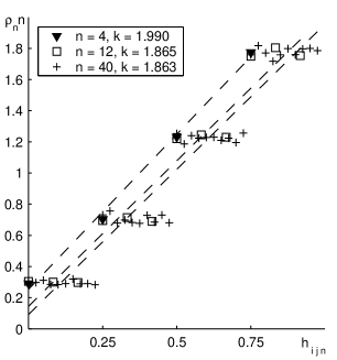
Figure 1: Normalized density of the heights; the dashed lines are the linear fits, $L=256$.

Each density is fitted by a linear function (fig. 1). The slopes slightly increase as $n$ goes up and must be saturating as $n$ tends to infinity.

The following construction manages to compare quantitatively four steps of $\rho_{n}(\cdot)$ as $n>4$ with the four values of $\rho_{4}(\cdot)$ representing BTW sand-pile. Given $n=4,5,\ldots$, the values of the density $\rho_{n}(\cdot)$ is sampled into four bins $[0,0.25)$, $[0.25,0.5)$, $[0.5,0.75)$, and $[0.75,1)$ with reported values $\psi_{n}(\cdot)$ at $0$, $0.25$, $0.5$, and $0.75$ respectively. For example, $\psi_{n}(0)=\rho_{n}(0)+\rho_{n}(1/n)+\ldots+\rho_{n}(j_{0}/n)$, where $j_{0}$ is the biggest integer with $j_{0}/n<0.25$. In particular, $\psi_{4}(\cdot)$ coincides with $\rho_{4}(\cdot)$. Then $\psi_{n}(\cdot)$ is defined in $4$ points. Each value $\psi(k/4)$, $k=0,1,2,3$, represents one step of $\rho_{n}(\cdot)$.

Let

$$\sigma_{n}=\left.\left(\sqrt{\sum_{k=0}^{3}\left(\psi_{n}(k/4)-\rho_{4}(k/4)\right)^{2}}\right)\,\right/3.$$

Then $\sigma_{n}$ measures the difference between the steps and the function $\rho_{4}(\cdot)$ corresponding to BTW sandpile.

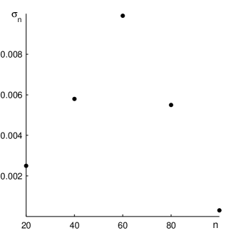
Figure 2: Difference between the steps of $\rho_{n}$ and the function $\rho_{4}$ measured by the functional $\sigma_{n}$.

The difference from BTW sand-pile increases as $\sigma_{n}$ goes up (fig. 2). The reported values of $\sigma_{n}$ indicate that there exist a certain maximum of the difference corresponding to $n\approx 60$. This observation agrees with the change of the tendency exhibited by the sand-pile family of Lübeck (2000b) for the intermediate values of the control parameter.

In the same way, the normalized densities are introduced to develop the models with $n\neq 4k$ starting with $n=3$. The computer experiment proves (fig. 3) that the densities $\rho_{n}$ quickly (as $n$ goes up) achieves four steps of $\rho_{4}$. The linear fits have slopes appearing close to that for $\rho_{4k}$.

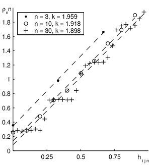
Figure 3: Normalized density of the heights; the dashed lines are the linear fits, $L=256$.

The following reasoning gives a rough explanation of the step-like behaviour of the densities. Given the parameter value $n$, the heights are naturally divided into four intervals $[H-n,H-3n/4)$, $[H-3n/4,H-n/2)$, $[H-n/2,H-n/4)$, $[H-n/4,H)$ since each act of relaxation maps one interval into another (possibly, excepting the boundary values due to the random effect). The normalization (on $n$) transforms these intervals to the domain of definition of four steps in fig. 1, and 3.

It worth noting that the sand-piles of Zhang (1989); Lübeck (2000b) demonstrate peaked densities of the average height in contrast to our $\rho_{n}$.

So, in terms of the sand distribution the model family exhibits a certain similarity. There exist possibilities to select the limit behaviour ($n\to\infty$) and define an intermediate deviation from the extreme cases. The densities $\rho_{n}$ for $n=4k$ and $n\neq 4k$ become almost indistinguishable as $n$ has the order of dozens.

IV Spectral approach

Another approach gives evidence of the diversity of the two cases ($n=4k$ and $n\neq 4k$). It deals with the spectrum of the average height $h=L^{-2}\sum_{i,j=1}^{L}h_{ij}$. The average height is calculated at the end of each time moment and treated as the function on time, $h(t)$. The paper de los Rios and Zhang (1999) has successfully used $h(t)$’s spectrum to describe the paper’s sand-pile’s dynamics. Our $h(t)$’s spectrum appears to be noisy, therefore it is averaged over its several realizations. Besides, each $h(t)$’s realization is stored in the bins of some length $\Delta$. Then the Fourier transform determines the spectrum $\xi$. The highest frequency is $1/\Delta$ in the case.

A formal procedure applied for the spectrum calculation consists of four steps.

1. For some fixed $N$ the time moments, which $h(t)$ is catalogued at, is divided into $N$ non-intersecting intervals of the same length $T$.

2. Given any fixed interval of step $1$, the averaging of $h(t)$-values over relatively small sub-intervals is applied to reduce the number of data for further numerical application of the fast Fourier transform. Let $\Delta$ be the length of the small sub-intervals and $r$ be their quantity, $r\Delta=T$. Then a signal $x_{j}$ is defined as the arithmetic mean of all the $h(t)$-values in the $j$-th small sub-interval, $j=1,2,\ldots,r$.

3. The Fourier transform determines the spectrum of $x_{j}$. Let

   $$\hat{x}_{k}=\frac{1}{\sqrt{r}}\sum_{j=1}^{r}\big{(}x_{j}-\langle x\rangle\big{)}e^{-\frac{2\pi ikj}{r}},$$

   where $\langle x\rangle$ is the mean of $x_{j}$, $j=1,\ldots,r$, $i=\sqrt{-1}$. Then the frequencies $f_{k}$ are $k/(r\Delta)$, $k=1,2,\ldots,r$, and the power spectrum $\xi(f_{k})$ of the signal $x_{j}$ is defined as $\xi(f_{k})=|\hat{x}_{k}|^{2}$.

4. Each of $N$ intervals defined in step $1$ generates its own spectrum $\xi(f_{k})$. The averaging of $\xi(f_{k})$ results in the stabilized spectrum, which the construction aims at. The stabilized spectrum depends on the model parameter $n$. Thus, the notation $\xi_{n}(f_{k})$ is keeping further for the stabilized spectrum.

According to Shapoval and Shnirman (2005), the family of the spectra admits a certain normalization. If $\Delta$ is proportional to $n$, the exhibition of $\xi_{n}(f_{k})/n$ versus dimensionless frequencies $f_{k}\Delta$ collapses the graphs on the interval of the high frequencies and remains reasonable on the other interval (fig. 4).

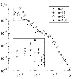
Figure 4: Normalized spectrum $\xi_{n}/n$ vs normalized frequencies $f=f_{k}$. The inset contains the graphs in the boxed part of the figure; $\Delta=8n$, $N=16$, $r=8192$, $L=256$.

Leaving the main part of the spectrum as it is we stress attention on some interval of the low frequencies. The corresponding part of the graphs is boxed in fig. 4 and put in its inset. In this part the graphs (for $n=4k$) establish a noticeable rise as $n$ goes up to the value being close to $60$. Then the tendency principally changes. The graphs turn down to the spectrum $\xi_{4}$ at their left part while demonstrating a definite peak (fig. 4, inset). It agrees with the behaviour of $\sigma_{n}$ reported earlier.

The spectrum’s propagation to the left needs much bigger $h(t)$’s domain of definition that is hardly possible. On the other hand, the highest achieved frequencies correspond to the avalanches of the biggest size observed during computer simulation. Bigger avalanches are practically not observable even for much longer simulation. Then the computer experiment must be producing the constant spectrum just at the left of the obtained graphs’ part in fig. 4.

The horizontal coordinates of the investigated box are not absolute constants. They depend on the lattice length $L$ and the simulation time. As $L$ increases the box moves to the left becoming invisible in fig. 4.

The influence of the simulation time is essential. The investigated part of the spectrum reflects the frequencies of the rare, big, and strongly dissipative avalanches. The lack of the data limits the results covering these avalanches. It concerns the partial conclusions about the rare avalanches in BTW’s and Manna’s sand-pile DeMenech et al. (1998).

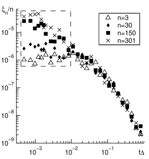
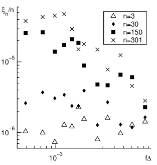
Figure 5: Normalized spectrum $\xi_{n}/n$ vs normalized frequencies $f=f_{k}$; $\Delta=8n$, $N_{R}=16$, $r=8192$, $L=256$ (a) full graph, (b) box of fig. a.

In contrast to the quick convergence of $\rho_{n}n$, $n\neq 4k$, to their four values, the family $\xi_{n}/n$ of the spectra exhibits quite a different tendency. Since the high-frequency spectra are rather similar (fig. 5a), the analysis is focused on the low frequencies (fig. 5b) corresponding to the boxed part in fig. 5a.

As $n=3$ the normalized spectrum has its horizontal interval. While $n$ increasing, $\xi_{n}/n$ changes on this interval. Fig. 5 demonstrates the minor changes as $n=30$ and completely another behaviour as $n$ is equal to $150$ and $301$. So, for the simulated big $n$s the low-frequency spectrum essentially deviates from $\xi_{3}$ as well as from $\xi_{4k}$ for big $k$.

According to fig. 4 and 5 the long-time evolution of the sand-pile exhibits a great complexity. In contrast to the space features, several patterns do not exhaust the spectrum behaviour. Up to the developed experiments the sand-piles with the deterministic and stochastic relaxation have the different spectra.

V Conclusion

Summarizing, we develop the family of the sand-piles. The control parameter $n$ is the number of the grains that any unstable cell passes to its neighbours. As $n=4k$, the propagation of the grains through the lattice is fully deterministic despite the models with $n\neq 4k$ involve some random effect. In terms of the sand distribution the random effect disappears as $n$ is sufficiently big. However the trace of the deterministic relaxation remains visible in terms of the average height’s spectrum, selecting some peak at low-frequency spectrum. With their peculiar evolutionary properties the sand-piles corresponding to the deterministic relaxation may admit a certain prediction. This hypothesis agrees with the effective precursors found for BTW’s sand-pile in Shapoval and Shnirman (2004).

References

- Bak et al. (1987) P. Bak, C. Tang, and K. Wiesenfeld, Phys. Rev. Lett. 59, 381 (1987).
- Bak et al. (1988) P. Bak, C. Tang, and K. Wiesenfeld, Phys. Rev. A 38, 364 (1988).
- Dhar (1990) D. Dhar, Phys. Rev. Lett. 64, 1613 (1990).
- Dhar (1999) D. Dhar, Physica A 263, 4 (1999).
- Grassberger and Manna (1990) P. Grassberger and S. S. Manna, J. Phys. (France) 51, 1077 (1990).
- Biham et al. (2001) O. Biham, E. Milshtein, and O. Malcai, Phys. Rev. E 63, 061309 (2001).
- Ktitarev et al. (2000) D. V. Ktitarev, S. Lübeck, P. Grassberger, and V. B. Priezzhev, Phys. Rev. E 61, 81 (2000).
- Miranda and J.Herrman (1991) E. N. Miranda and H. J.Herrman, Phys. A 175, 339 (1991).
- Bak and Tang (1987) P. Bak and C. Tang, J. Geophysical Res. 94, 15635 (1987).
- Bershadskii and Sreenivasan (2003) A. Bershadskii and K. R. Sreenivasan, Eur. Phys. J. B 35, 513 (2003).
- Manna (1990) S. S. Manna, J. Stat.Phys. 59, 509 (1990).
- Zhang (1989) Y.-C. Zhang, Phys. Rev. Lett. 63, 470 (1989).
- Ben-Hur and Biham (1996) A. Ben-Hur and O. Biham, Phys. Rev. E 53, R1317 (1996).
- Pietronero et al. (1994) L. Pietronero, A. Vespignani, and S.Zapperi, Phys. Rev. Lett. 72, 1690 (1994).
- Chessa et al. (1999) A. Chessa, H. E. Stanley, A. Vespignani, and S. Zapperi, Phys. Rev. E 59, R12 (1999).
- Ivashkevich et al. (1999) E. V. Ivashkevich, A. M. Povolotsky, A. Vespignani, and S. Zapperi, Phys. Rev. E 60, 1239 (1999).
- Tebaldi et al. (1999) C. Tebaldi, M. DeMenech, and A. L. Stella, Phys. Rev. Lett. 83, 3952 (1999).
- Lübeck (2000a) S. Lübeck, Phys. Rev. E 61, 204 (2000a).
- Lübeck and Usadel (1997) S. Lübeck and K. D. Usadel, Phys. Rev. E 55, 4095 (1997).
- Lübeck (2000b) S. Lübeck, Phys. Rev. E 62, 6149 (2000b).
- Shapoval and Shnirman (2005) A. B. Shapoval and M. G. Shnirman, IJMPC 16 (2005).
- de los Rios and Zhang (1999) P. de los Rios and Y. Zhang, Phys. Rev. 82, 472 (1999).
- Karmakar et al. (2005) R. Karmakar, S. S. Manna, and A. L. Stella, Phys. Rev. Lett. 94, 088002 (2005).
- Priezzhev (1994) V. B. Priezzhev, J. Stat. Phys. 74, 955 (1994).
- DeMenech et al. (1998) M. DeMenech, A. L. Stella, and C. Tebaldi, Phys. Rev. E 58, R2677 (1998).
- Shapoval and Shnirman (2004) A. B. Shapoval and M. G. Shnirman, IJMPC 15, 279 (2004).