Inverse swelling of a hydrophobic polymer in aqueous solution

Abstract

We address the problem of inverse polymer swelling. This phenomenon, in which a collapsed polymer chain swells upon decreasing temperature, can be observed experimentally in so-called thermoreversible homopolymers in aqueous solution, and is believed to be related to the role of hydrophobicity in protein folding. We consider a lattice-fluid model of water, defined on a body-centered cubic lattice, which has been previously shown to account for most thermodynamic anomalies of water and of hydrophobic solvation for monomeric solutes. We represent the polymer as a self-avoiding walk on the same lattice, and investigate the resulting model at a first order approximation level, equivalent to the exact calculation on a Husimi lattice. Depending on interaction parameters and applied pressure, the model exhibits first and/or second order swelling transitions upon decreasing temperature.

I Introduction

From the experimental point of view, water is known to exhibit several thermodynamic anomalies, both as a pure substance Franks (1982); Stanley et al. (2003) and as a solvent, in particular for non-polar (hydrophobic) chemical species Ben-Naim (1980); Dill (1990a); Southall et al. (2002). The transfer process of a small non-polar solute molecule in water is characterized by a positive solvation Gibbs free energy (it is thermodynamically unfavored), a negative solvation enthalpy (it is energetically favored), a negative solvation entropy (it has an ordering effect), and a large positive solvation heat capacity Ben-Naim (1987). More precisely, for prototype hydrophobic species (that is, for instance, noble gases), solvation entropies and enthalpies, which are negative at room temperature, increase upon increasing temperature, and eventually become positive. Accordingly, the solvation Gibbs free energy displays a maximum as a function of temperature. These properties define the so-called hydrophobic effect.

It is quite well established that the hydrophobic effect is an important driving force for several biophysical processes Tanford (1980), and in particular for protein folding Dill (1990b). This is the reason why it has attracted a high degree of attention in the last years, but a unified theoretical framework for this phenomenon does not exist yet. It has been observed that the native folded state of proteins is maximally stable in the range of temperatures of living organisms, whereas it tends to be destabilized both by increasing and by decreasing temperature. For globular proteins, it is eventually possible to observe complete denaturation also upon decreasing temperature Privalov (1990); Makhatadze and Privalov (1995). This phenomenon is denoted as cold unfolding, and has a simple analogue in so-called thermoreversible homopolymers, which exhibit a transition from a collapsed to a swollen state, upon decreasing temperature Tiktopulo et al. (1995); Wu and Zhou (1996); Wu and Wang (1998). We denote this kind of phase transition as inverse swelling. All this phenomenology is qualitatively consistent with the previously mentioned existence of a maximum in the stabilizing force, i.e., hydrophobic repulsion, as a function of temperature. Such reasoning is of course unrigorous, since the hydrophobic effect is not a real interaction, but an effective repulsion, resulting from an average over the degrees of freedom of water.

Cold unfolding and inverse swelling have attracted some attention from the theoretical point of view Hansen et al. (1998, 1999); Bakk et al. (2001a, b); Rios and Caldarelli (2000, 2001); Bruscolini and Casetti (2000, 2001); Bruscolini et al. (2001, 2002), and they have been a starting point for highlighting the importance of water structure details for modeling protein folding Salvi and Rios (2003). One possible way of investigation consists of computer simulations, based on very detailed (all-atom) interaction potentials. Unfortunately, simulations are generally limited by the large computational effort required. Investigation of a full protein model with explicit water is still out of reach Paschek and Garcìa (2004), and also for homopolymers the analysis is generally limited to relatively short chains or small parameter regions Polson and Zuckermann (2000); Ghosh et al. (2005); Paschek et al. (2005). A complementary approach involves investigations of simplified models, either on- or off-lattice. Several models of this kind have been proposed Hansen et al. (1998, 1999); Bakk et al. (2001a, b); Rios and Caldarelli (2000, 2001); Bruscolini and Casetti (2000, 2001); Bruscolini et al. (2001, 2002). As previously mentioned, it turns out that, in order to reproduce inverse swelling (or cold unfolding), it is necessary to take into account, even in extremely simplified fashions, the degrees of freedom of water. Nevertheless, such descriptions are generally proposed ad-hoc for this kind of problem. The focus is mainly on the polymer, whereas water models by themselves would not be satisfactory models of water.

Conversely, in this article, we start by considering a lattice-fluid model of water, whose thermodynamic properties have been previously investigated in detail Pretti and Buzano (2004, 2005). This model predicts most of the thermodynamic anomalies of real water at constant pressure (a temperature of maximum density, a minimum of isothermal compressibility and specific heat), and also a liquid-liquid phase separation in the supercooled region, and a second critical point Pretti and Buzano (2004). Moreover, a corresponding model for aqueous solutions of ideally inert monomeric solutes turns out to exhibit the above mentioned fingerprints of hydrophobicity, and in particular the maximum in the solvation free energy as a function of temperature Pretti and Buzano (2005). We describe the polymer in solution as a lattice self-avoiding walk, whose steps connect nearest neighbor sites. We assume that each visited site, representing a monomeric unit, interacts with water and with other non-consecutive monomeric units, in the same way as the elementary solute of the the original model does. In some sense, our model is unbiased.

The water model is a simplified version of the one proposed by Roberts and Debenedetti Roberts and Debenedetti (1996); Roberts et al. (1996, 1998). It is defined on the body-centered cubic lattice, and water molecules possess four equivalent bonding arms arranged in a tetrahedral symmetry. According to this model, the microscopic description of water anomalies is based on the competition between an isotropic (van der Waals-like) interaction and a highly directional (hydrogen bonding) interaction, and on the difference between the respective optimal interaction distances. In the lattice environment, the latter is taken into account by a trick, that is, a weakening of hydrogen bonds by neighboring water molecules.

The previously mentioned results on this model have been obtained by a first order approximation on a tetrahedral cluster (equivalent to the exact calculation for a Husimi lattice Pretti (2003) made up of tetrahedral building blocks), but turn out to compare quite well with Monte Carlo simulations Pretti and Buzano (2004). The same kind of approximation has been independently verified to be rather accurate for the case of a semiflexible self-interacting polymer chain Pretti (2002) with no explicit solvent. We thus expect that the calculation presented here, based on the same approximation technique, could produce reliable results as well, although it is being applied to a more complicated model involving water-polymer interactions.

II The model

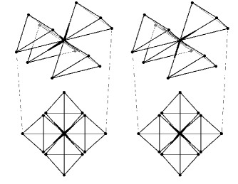
Figure 1: Husimi lattice structure and bonding water configurations $i=1$ (left) and $i=2$ (right). Views from top are meant to explain configuration symbols used in Table 1.

Let us now describe the model in detail. As previously mentioned, it is defined on the bcc lattice. Each site may be empty or occupied by a water molecule ($\mathsf{w}$) or by a polymer segment ($\mathsf{s}$). Since we find it more convenient to work in the grand-canonical ensemble, each of the two species contributes to the hamiltonian by a different chemical potential term $-\mu_{\mathsf{x}}$, where $\mathsf{x}\in\{\mathsf{w},\mathsf{s}\}$. An attractive (Van der Waals) energy $-\epsilon_{\mathsf{x}\mathsf{y}}<0$ is assigned to any pair of nearest neighbor (NN) sites occupied by $\mathsf{x},\mathsf{y}$ molecules, where $\mathsf{x}$ and $\mathsf{y}$ run over $\{\mathsf{w},\mathsf{s}\}$. Of course, the interaction energy between polymer segments $-\epsilon_{\mathsf{s}\mathsf{s}}$ is taken into account only if the segments are not consecutive along the chain. Water molecules possess four equivalent arms that can form hydrogen bonds, arranged in a tetrahedral symmetry, so that they can point towards 4 out of 8 NNs of a given site. A hydrogen bond is formed whenever two NN molecules have a bonding arm pointing to each other, yielding an energy $-\eta<0$. Only 2 different water configurations can form hydrogen bonds (see Fig. 1); $w$ more configurations are allowed, in which water molecules cannot form bonds (the $w$ parameter is related to the bond-breaking entropy). An energy increase $\eta c_{\mathsf{x}}/6$, with $c_{\mathsf{x}}\in[0,1]$, is added for each of the $6$ sites closest to a bond (i.e., 3 out of 6 next nearest neighbors of each bonded molecule), occupied by an $\mathsf{x}$ molecule. As far as water molecules are concerned, the weakening parameter mainly accounts for the fact that hydrogen bonds are most favorably formed when water molecules are located at a certain distance, larger than the optimal Van der Waals distance. Therefore, if too many molecules are present, the average distance among them decreases, and hydrogen bonds are (on average) weakened. Moreover, the presence of an external molecule may perturb the electronic density, resulting in a lowered hydrogen bond strength as well. A weakening parameter $c_{\mathsf{s}}$ for polymer segments could take into account possible perturbation effects for a generic chemical species. Nevertheless, in this paper we shall consider only the case of an ideal monomer with $c_{\mathsf{s}}=0$.

The bcc lattice model can be conveniently replaced by an analogous model defined on a Husimi lattice made up of irregular tetrahedral building blocks (see Fig. 1), as explained in detail in Refs. Pretti and Buzano, 2004 and Pretti and Buzano, 2005. The latter model, which can be studied exactly, is equivalent to a generalized first order approximation (on the tetrahedral cluster) for the original model Pretti (2003). From now on, we shall refer to the Husimi lattice model only. The hamiltonian of the system can be written as a sum over the tetrahedral clusters

$$\mathcal{H}=\sum_{\langle\alpha,\beta,\gamma,\delta\rangle}\mathcal{H}_{i_{\alpha}i_{\beta}i_{\gamma}i_{\delta}},$$ (1)

where $\mathcal{H}_{ijkl}$ is the contribution of each cluster, which will be referred to as tetrahedron hamiltonian, and the subscripts $i_{\alpha},i_{\beta},i_{\gamma},i_{\delta}$ label site configurations for the $4$ vertices ($\alpha,\beta,\gamma,\delta$). It is understood that the latter are enumerated in a conventional order, for instance clockwise, with reference to Fig. 1 (bottom). Accordingly, $(\alpha,\beta)$, $(\beta,\gamma)$, $(\gamma,\delta)$, and $(\delta,\alpha)$ turn out to be NN pairs, whereas $(\alpha,\gamma)$ and $(\beta,\delta)$ are next nearest neighbors.

Site configurations are reported in Table 1, where $i=1,2,3$ denote water molecule configurations (defined as in Refs. Pretti and Buzano, 2004, 2005) and $i=4,\dots,8$ denote local configurations of the polymer chain. As far as polymer configurations are concerned, let us notice that they are more conveniently defined with respect to the tetrahedron, than with respect to a fixed reference frame. This trick allows us to write a unique form for the tetrahedron hamiltonian, which otherwise would be orientation-dependent. Moreover, although in the isotropy hypothesis every local chain configuration should be equally probable, we need to distinguish different classes of configurations (each one with a given multiplicity) in order to impose connectivity constraints, as it will be clarified below. As a consequence, the Husimi lattice approximation introduces a small artifact, in that the probability of the configurations $i=4,6$ (in which the chain locally stays in the same cluster) turns out to be slightly different from the probability of the configurations $i=5,7,8$ (in which the chain passes from one cluster to another). We expect that such artifact is negligible, according to the results of Ref. Pretti, 2002.

The tetrahedron hamiltonian can be written as

$$\mathcal{H}_{ijkl}=H_{ijkl}+H_{jkli}+H_{klij}+H_{lijk}+L_{ijkl},$$ (2)

where

$$H_{ijkl} = -\epsilon_{\mathsf{xy}}{n_{\mathsf{x},{i}}}{n_{\mathsf{y},{j}}}\,\overline{b_{i}^{+}b_{j}^{-}}-\eta h_{ij}\left(1-c_{\mathsf{x}}\frac{{n_{\mathsf{x},{k}}}+{n_{\mathsf{x},{l}}}}{2}\right)$$ (3)

$$-\frac{1}{4}\mu_{\mathsf{x}}{n_{\mathsf{x},{i}}}+I\left(b_{i}^{+}\oplus b_{j}^{-}\right).$$

Let us analyze the various terms appearing in these equations.

The first line of Eq. (3) is basically equivalent to the corresponding term for the mixture model of water and a simple monomeric solute [see Eq. (3) in Ref. Pretti and Buzano, 2005], and includes the Van der Waals and the hydrogen bonding terms. Occupation variables ${n_{\mathsf{x},{i}}}$ are defined as ${n_{\mathsf{x},{i}}}=1$ if the configuration $i$ corresponds to a chemical species $\mathsf{x}$, and ${n_{\mathsf{x},{i}}}=0$ otherwise (see Table 1), whereas $h_{ij}$ are hydrogen bond variables, defined as $h_{ij}=1$ if the pair configuration $(i,j)$ represents a hydrogen bond (i.e., if $i=1$ and $j=2$), and $h_{ij}=0$ otherwise. It is understood that repeated $\mathsf{x}$ and $\mathsf{y}$ indices are summed over their possible values $\mathsf{w},\mathsf{s}$. The only difference with respect to the monomeric solute case is related to the fact that, as previously mentioned, we have to exclude Van der Waals interactions between consecutive polymer segments. To do so, we have defined the bond numbers $b_{i}^{+}$ (resp. $b_{i}^{-}$), which are boolean variables equal to $1$ if the configuration $i$ represents a polymer segment forming a chemical bond in the clockwise (resp. counterclockwise) direction of the reference cluster, and $0$ otherwise (see Table 1). In this way, the multiplying term $\overline{b_{i}^{+}b_{j}^{-}}$ (where the overline denotes boolean negation) is $0$ if $(i,j)$ represents two consecutive segments, and $1$ otherwise.

The second line of Eq. (3) includes the chemical potential contributions (multiplied by $1/4$ to avoid overcounting) and an infinite energy penalty $I\to\infty$, assigned to $(i,j)$ configurations which violate connectivity constraint, i.e., when $i$ wants to form a chemical bond (in the clockwise direction) and $j$ does not (in the counterclockwise direction), or vice versa. This is obtained by the exclusive-or factor $\left(b_{i}^{+}\oplus b_{j}^{-}\right)$. Let us notice that the infinite energy penalty can be treated numerically, since we have to deal only with Boltzmann factors of the tetrahedron hamiltonian. Finally, the additive term $L_{ijkl}$ in Eq. (2) is another constraint term, needed to forbid short loops on tetrahedra. It is therefore simply defined as $L_{6666}=\infty$ and $L_{ijkl}=0$ otherwise.

Table 1: Site configurations, with corresponding labels ($i$), multiplicities ($w_{i}$), occupation variables (${n_{\mathsf{w},{i}}},{n_{\mathsf{s},{i}}}$), and chemical bond numbers ($b_{i}^{+},b_{i}^{-}$). Polymer configurations are defined with reference to the cluster denoted by a dot; $i^{\prime},i^{\prime\prime},i^{\prime\prime\prime}$ denote the configurations “viewed” by the other $3$ clusters: $i=0$ empty site; $i=1,2$ bonding water; $i=3$ non-bonding water; $i=4$ segments in the same cluster, out of the reference one; $i=5$ segments in different clusters, out of the reference one; $i=6$ segments in the same cluster, the reference one; $i=7$ segments in different clusters, one in the reference cluster (“clockwise” direction); $i=8$ segments in different clusters, one in the reference cluster (“counterclockwise” direction);

$i$	$0$	$1$	$2$	$3$	$4$	$5$	$6$	$7$	$8$
$i^{\prime}$	$0$	$1$	$2$	$3$	$6$	$5$	$4$	$8$	$7$
$i^{\prime\prime}$	$0$	$1$	$2$	$3$	$4$	$7$	$4$	$5$	$5$
$i^{\prime\prime\prime}$	$0$	$1$	$2$	$3$	$4$	$8$	$4$	$5$	$5$
$w_{i}$	$1$	$1$	$1$	$w$	$3$	$12$	$1$	$6$	$6$
${n_{\mathsf{w},{i}}}$	$0$	$1$	$1$	$1$	$0$	$0$	$0$	$0$	$0$
${n_{\mathsf{s},{i}}}$	$0$	$0$	$0$	$0$	$1$	$1$	$1$	$1$	$1$
$b_{i}^{+}$	$0$	$0$	$0$	$0$	$0$	$0$	$1$	$1$	$0$
$b_{i}^{-}$	$0$	$0$	$0$	$0$	$0$	$0$	$1$	$0$	$1$

III The first order (Husimi lattice) approximation

As mentioned in the Introduction, we perform the exact analysis of the Husimi lattice model, which is equivalent to the generalized first order approximation on tetrahedral clusters. The calculation closely follows the one of the ordinary mixture model, performed in Ref. Pretti and Buzano, 2005, so that we do not give much detail. Basically, one has to take into account that the system is locally tree-like, which allows to write a recursion equation Pretti (2003), for so-called partial partition functions, defined as follows. Let us assume that the lattice is actually a tree (Husimi tree), and let us consider just one branch, with the corresponding partial hamiltonian, obtained by Eq. (1) with the sum restricted to tetrahedra in the branch. The partial partition function $Q_{i}$ is a sum of Boltzmann weights of the partial hamiltonian, taken over the configurations of the branch except the base site (this is why the partial partition function depends on the base site configuration variable $i$). It is convenient to define normalized partial partition functions $q_{i}\propto Q_{i}$, for instance in such a way that

$$\sum_{i=0}^{8}q_{i}=1.$$ (4)

If the branch becomes infinite, i.e., in the thermodynamic limit, and in the homogeneity hypothesis, the subbranches attached to the first tetrahedral cluster are equivalent to the main one, so that one can write the recursion equation

$$q_{i}=y^{-1}\sum_{j=0}^{8}w_{j}\sum_{k=0}^{8}w_{k}\sum_{l=0}^{8}w_{l}e^{-\mathcal{H}_{ijkl}/T}\prod_{\xi=\prime}^{\prime\prime\prime}q_{j^{\xi}}q_{k^{\xi}}q_{l^{\xi}},$$ (5)

where the sum runs over configuration variables in the tetrahedron except $i$, $T$ is the temperature expressed in energy units, and $y$ is a normalization constant.

Let us notice a subtle but important difference with respect to the corresponding equation for the monomeric solute [Eq. (8) in Ref. Pretti and Buzano, 2005]. As mentioned in the previous section, we have defined local chain configurations with reference to a given cluster, which allows us to write one single tetrahedron hamiltonian, independently of orientation. Therefore, when we consider the operation of “attaching branches” to a base cluster, we have to take into account configurations of sites in the cluster as they are “viewed” by the attached branches. To do so, we have to write a product over $\xi=\prime,\prime\prime,\prime\prime\prime$, which denote precisely the different views, according to Table 1.

The recursion equation can be iterated numerically to determine a fixed point. The site configuration probabilities $p_{i}$ can be computed by considering the operation of attaching $4$ branches to the given site, yielding

$$p_{i}=z^{-1}q_{i}\prod_{\xi=\prime}^{\prime\prime\prime}q_{i^{\xi}},$$ (6)

where the normalization constant is determined as

$$z=\sum_{i=0}^{8}w_{i}q_{i}\prod_{\xi=\prime}^{\prime\prime\prime}q_{i^{\xi}}.$$ (7)

From the knowledge of site configuration probabilities $p_{i}$, one can easily compute the densities, i.e., the probabilities $\rho_{\mathsf{w}},\rho_{\mathsf{s}}$ that a site is occupied by a water molecule or by a polymer segment, respectively. For $\mathsf{x}\in\{\mathsf{w},\mathsf{s}\}$, we have

$$\rho_{\mathsf{x}}=\sum_{i=0}^{8}w_{i}p_{i}{n_{\mathsf{x},{i}}},$$ (8)

where the occupation numbers ${n_{\mathsf{x},{i}}}$ are explicitly given in Table 1.

In the presence of multiple fixed points (which can be reached from different initial conditions), i.e., in the presence of coexistence phenomena, the first order transition can be determined by minimizing the (grand-canonical) free energy per site

$$\omega=-T\left(\ln y-2\ln z\right),$$ (9)

where $y$ and $z$ are the normalization constants of the recursion equation and of the site probability distribution, respectively. The derivation of this expression requires some manipulations, and is left to the Appendix. From the knowledge of the free energy, one can in principle compute all other thermodynamic properties. Assuming the volume per site equal to $1$, pressure can be expressed in energy units as $P=-\omega$.

IV Results

First of all, we have to fix a set of model parameters. As far as water is concerned, we choose the values of our previous investigation Pretti and Buzano (2004): $\epsilon_{\mathsf{ww}}/\eta=0.25$, $w=20$, and $c_{\mathsf{w}}=0.5$. The hydrogen bond energy $\eta$ is taken as the energy unit. The water-water van der Waals energy $\epsilon_{\mathsf{ww}}$ is significantly smaller. The multiplicity $w$ of non-bonding water configurations is large, to mimic the high directionality of hydrogen bonds.

With this set of parameters, the model provides a qualitatively consistent description of the phase diagram and thermodynamic anomalies of pure water Pretti and Buzano (2004), as already mentioned in the Introduction. For the liquid phase, one observes a density maximum as a function of temperature at fixed pressure, i.e., a change of sign in the isobaric thermal expansion coefficient

$$\alpha_{P}=-\frac{\partial\ln\rho_{\mathsf{w}}}{\partial T}\biggr{\lvert}_{P}.$$ (10)

The temperature of maximum density slightly decreases upon increasing pressure, as observed in experiments. The isothermal compressibility

$$\kappa_{T}=\frac{\partial\ln\rho_{\mathsf{w}}}{\partial P}\biggr{\lvert}_{T}$$ (11)

and the isobaric specific heat exhibit a minimum as a function of temperature, at constant pressure. Moreover, in the supercooled regime, the model predicts the so-called second critical point, which has been conjectured and observed in simulations Stanley et al. (2003), and of which also some experimental evidences have been found Mishima and Stanley (1998). The liquid-vapor spinodal displays no reentrance in the positive pressure half-plane, whereas the temperature of maximum density locus exhibits a peculiar “nose-shaped” reentrance. Let us recall that this scenario qualitatively agrees with recent molecular dynamics simulations of water phenomenological potentials in the negative pressure region Stanley et al. (2003), whereas the reentrant spinodal scenario is an older conjecture invoked to explain thermodynamic anomalies of liquid water Speedy (1982); Zheng et al. (1991). The plausibility of the latter has been recently a matter of debate Speedy (2004); Debenedetti (2004), but seems to be definitely ruled out.

We summarize the results obtained by our model for pure water in Fig. 2 (phase diagram) and Fig. 3 (response functions), in order to delimit the temperature range in which we ought to expect the (stable or metastable) liquid water regime. Let us notice that the response functions correctly exhibit a divergent behavior, upon approaching the liquid phase spinodal.

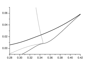
Figure 2: Pressure ($P/\eta$) vs temperature ($T/\eta$) phase diagram for pure water. The solid line denotes the liquid-vapor transition line, the thin solid line denotes the liquid phase spinodal, whereas the thin dotted line denotes the temperature of maximum density locus. Parameter values: $\epsilon_{\mathsf{ww}}/\eta=0.25$, $w=20$, $c_{\mathsf{w}}=0.5$.

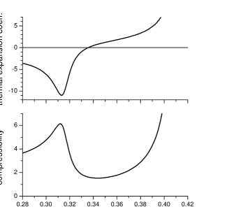
Figure 3: Pure water response functions at fixed pressure ($P/\eta=0.05$) as a function of temperature ($T/\eta$). Upper graph: isobaric thermal expansion coefficient ($\eta\alpha_{P}$). Lower graph: isothermal compressibility ($\eta\kappa_{T}$). Parameter values: $\epsilon_{\mathsf{ww}}/\eta=0.25$, $w=20$, $c_{\mathsf{w}}=0.5$.

Upon inserting an ideal inert solute, i.e., adding a monomeric $\mathsf{s}$ chemical species, characterized by $\epsilon_{\mathsf{ws}}=\epsilon_{\mathsf{ss}}=0$ and $c_{\mathsf{s}}=0$, we have shown that the model is able to reproduce in a qualitatively accurate way also the solvation properties of simple hydrophobic solutes, such as noble gases Pretti and Buzano (2005). Since in Ref. Pretti and Buzano, 2005 we have not considered the present set of water parameters, we report here the results, in terms of solvation free energy, entropy, and enthalphy as a function of temperature (Fig. 4).

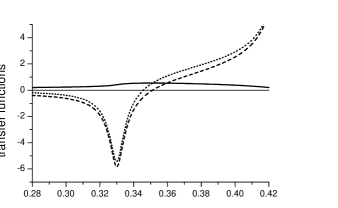
Figure 4: Transfer energy functions ($E/\eta$) vs temperature ($T/\eta$) for a single monomer at liquid-vapor coexistence: $E=\Delta g^{*}$ (solid line), $E=T\Delta s^{*}$ (dashed line), $E=\Delta h^{*}$ (dotted line). Parameter values: $\epsilon_{\mathsf{ww}}/\eta=0.25$, $w=20$, $c_{\mathsf{w}}=0.5$, $\epsilon_{\mathsf{ws}}=\epsilon_{\mathsf{ss}}=0$, $c_{\mathsf{s}}=0$.

The solvation Gibbs free energy per molecule $\Delta g^{*}$, i.e., the transfer free energy of a solute molecule from vapor to liquid phase at coexistence, can be computed as

$$\Delta g^{*}=-T\ln\frac{\rho_{\mathsf{s}}^{(\mathrm{l})}}{\rho_{\mathsf{s}}^{(\mathrm{v})}},$$ (12)

where $\rho_{\mathsf{s}}^{(\mathrm{v})}$ and $\rho_{\mathsf{s}}^{(\mathrm{l})}$ denote solute densities in the two phases, respectively. The solvation entropy is defined as

$$\Delta s^{*}=-\frac{\partial\Delta g^{*}}{\partial T}\biggr{\lvert}_{P},$$ (13)

and the solvation enthalpy can then be computed as

$$\Delta h^{*}=\Delta g^{*}+T\Delta s^{*}.$$ (14)

The typical experimental temperature range for several hydrophobic compounds is around $0^{\circ}\mathrm{C}$ to $300^{\circ}\mathrm{C}$ Ben-Naim (1987). According to pure water results, in our model this roughly corresponds to the range $T/\eta\approx 0.33$ (just below the temperature of maximum density) to $T/\eta\approx 0.38$ (about half way between the previous temperature and the critical temperature). In this range, the solvation Gibbs free energy is positive and displays a broad maximum, whereas entropy and enthalpy are negative at low temperatures and positive at high temperatures, in agreement with experiments Ben-Naim (1987). Upon approaching the critical point, the free energy tends to zero, whereas the entropy and enthalphy diverge.

For the polymeric solute, we carry out the investigation as discussed in the previous Section. We compute, as a composition variable, the segment molar fraction, defined as

$$x=\frac{\rho_{\mathsf{s}}}{\rho_{\mathsf{w}}+\rho_{\mathsf{s}}}.$$ (15)

We perform the analysis at constant pressure $P/\eta=0.05$, i.e., the same value for which we have computed pure water response functions. At fixed temperature, we always observe a transition between a phase with $x=0$ (pure water) at lower values of the segment chemical potential $\mu_{\mathsf{s}}$, and another phase with a certain positive fraction $x$ of polymer segments (polymerized phase) at higher $\mu_{\mathsf{s}}$ values. In order to determine this transition, we have programmed a numerical procedure, which adjusts the water chemical potential $\mu_{\mathsf{w}}$ in order to fix the pressure of the two phases, and then finds the $\mu_{\mathsf{s}}$ transition value, at which the water chemical potentials of the two phases are equal. The polymerized phase at the transition describes the behavior of an isolated polymer chain in solution Vanderzande (1998). Accordingly, the $x$ value at this point is an indicator of the polymer chain compactness, as a function of temperature. If $x=0$, the transition is continuous, and the polymer is in a completely swollen state, whereas, if $x>0$, the transition is first order, and the polymer is in a more or less collapsed state.

As far as interaction parameters are concerned, we have first investigated a completely inert (hydrophobic) polymer, assuming $\epsilon_{\mathsf{ws}}=\epsilon_{\mathsf{ss}}=0$ and $c_{\mathsf{s}}=0$, and then we have turned on a slight attractive water-segment interaction ($\epsilon_{\mathsf{ws}}>0$). Depending on the value of this parameter, we have obtained different interesting behaviors. The results are summarized in Figs. 5 and 6.

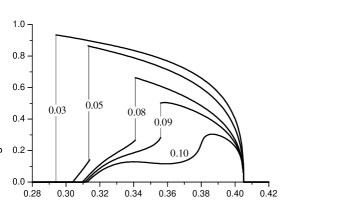
Figure 5: Polymer compactness (segment molar fraction $x$ for the polymerized phase at the transition with the pure water phase) as a function of temperature ($T/\eta$) at fixed pressure ($P/\eta=0.05$), for different values of $\epsilon_{\mathsf{ws}}/\eta$ (reported on each plot). Other parameter values: $\epsilon_{\mathsf{ww}}/\eta=0.25$, $w=20$, $c_{\mathsf{w}}=0.5$, $\epsilon_{\mathsf{ss}}=0$, $c_{\mathsf{s}}=0$.

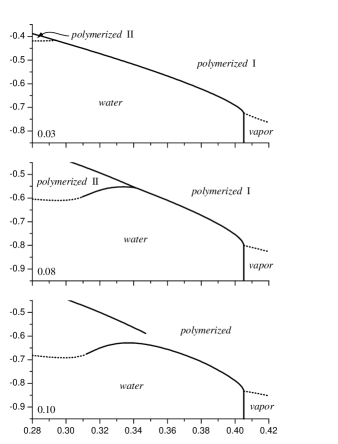
Figure 6: Segment chemical potential ($\mu_{\mathsf{s}}/\eta$) vs temperature ($T/\eta$) phase diagrams at fixed pressure ($P/\eta=0.05$), for different values of $\epsilon_{\mathsf{ws}}/\eta$ (reported on each graph). Other parameter values: $\epsilon_{\mathsf{ww}}/\eta=0.25$, $w=20$, $c_{\mathsf{w}}=0.5$, $\epsilon_{\mathsf{ss}}=0$, $c_{\mathsf{s}}=0$. Solid and dashed lines denote first and second order transitions, respectively.

From $\epsilon_{\mathsf{ws}}=0$ to $\epsilon_{\mathsf{ws}}/\eta\approx 0.04$, we observe a first-order inverse swelling, since the segment molar fraction $x$ abruptly jumps from a high value down to zero (Fig. 5). In the $\mu_{\mathsf{s}}$ vs $T$ phase diagram (Fig. 6, top panel), this transition corresponds to a critical end-point, which lies among two different polymerized phases with different densities, and the water phase. Upon decreasing the segment chemical potential $\mu_{\mathsf{s}}$, the low temperature polymerized phase undergoes a second order transition to the pure water phase, corresponding to the swollen state. On the contrary, the high temperature polymerized phase undergoes a first order transition to the pure water phase, corresponding to the collapsed state. For $\epsilon_{\mathsf{ws}}=0$, the inverse swelling transition occurs around $T/\eta\approx 0.227$. At such a low temperature, we expect that the liquid water phase predicted by our model is actually unstable, so that the observed phase behavior is to be viewed as an extrapolation Pretti and Buzano (2004). Upon increasing $\epsilon_{\mathsf{ws}}$, the inverse swelling transition temperature increases. It is interesting to notice that also an “ordinary” swelling transition can be observed at high temperature. Such transition coincides with the liquid-vapor transition of pure water, and it is therefore completely unaffected by the water-segment interaction parameter $\epsilon_{\mathsf{ws}}$. In our opinion, such feature is a clear evidence that the polymer collapse is induced by the presence of a dense (liquid) aqueous solvent around it, i.e., by the hydrophobic effect.

For $\epsilon_{\mathsf{ws}}/\eta\gtrsim 0.04$, the behavior changes, in that inverse swelling occurs via an intermediate, moderately collapsed phase (Fig. 5). Upon decreasing temperature, we first observe a discontinuous jump of the segment molar fraction $x$ from a high value to a smaller value, and subsequently a continuous transition to a completely swollen state with $x=0$. In the $\mu_{\mathsf{s}}$ vs $T$ phase diagram (Fig. 6, middle panel), the former transition corresponds to a triple point among the two polymerized phases and the water phase. The latter transition corresponds to a “tricritical” point, at which the transition between the low temperature polymerized phases and the pure water phase changes from first to second order. Such behavior resembles a $\Theta$ point Vanderzande (1998) in which the role of temperature is reversed. Upon increasing $\epsilon_{\mathsf{ws}}$, the temperatures of both transitions increase, and the amplitude of the discontinuous one is progressively reduced.

Around $\epsilon_{\mathsf{ws}}/\eta\approx 0.10$, we observe a totally continuous inverse swelling, but a reminiscence of the first order jump can still be observed (Fig. 5). Such a behavior corresponds, in the $\mu_{\mathsf{s}}$ vs $T$ phase diagram (Fig. 6, bottom panel), to the fact that the transition between the two different polymerized phases ends in a critical point before encountering the transition line with the pure water phase. For $\epsilon_{\mathsf{ws}}/\eta\approx 0.11$ and above, we can no longer observe a collapsed phase, and the polymer is completely swollen at all temperatures. Accordingly, in the $\mu_{\mathsf{s}}$ vs $T$ phase diagram, the transition between the polymerized phase and the pure water phase is second order at all temperatures.

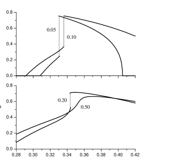
Figure 7: Polymer compactness (segment molar fraction $x$ for the polymerized phase at the transition with the pure water phase) as a function of temperature ($T/\eta$), for different pressure values $P/\eta$ (reported on each plot). Parameter values: $\epsilon_{\mathsf{ww}}/\eta=0.25$, $w=20$, $c_{\mathsf{w}}=0.5$, $\epsilon_{\mathsf{ws}}/\eta=0.07$, $\epsilon_{\mathsf{ss}}=0$, $c_{\mathsf{s}}=0$.

It is noticeable that the effect of pressure on the polymer behavior is somehow similar to the effect of the water-segment attractive energy $\epsilon_{\mathsf{ws}}$, as shown in Fig. 7. The first-order swelling transition temperature increases upon increasing pressure. The transition becomes less and less abrupt, and is finally smoothed out at high pressure values, i.e., in the pressure vs temperature phase diagram, the transition line ends in a critical point. Let us notice, by the way, that a similar critical behavior has been predicted by a simplified model of cold unfolding for proteins Hansen et al. (1999).

We can also observe some differences. For instance, the high temperature swelling transition, which was unaffected by the water-segment interaction at fixed pressure, increases upon increasing pressure, although, at pressure values lower than the critical one, it still coincides with the liquid-vapor transition. This means that indeed, at high temperature, pressure tends to make the polymer coil more compact. The same holds true for the low temperature, moderately collapsed phase. This effect is reversed at very high pressures.

It is important to stress that the different polymer behaviors described above partially occur in a temperature region which is likely to be unreachable by experiments. According to Fig. 3, the response functions of pure water display peaks, but in actual experiments only their high temperature “sides” can be observed. The real peaks are believed to lie below the homogeneous nucleation temperature Stanley et al. (2003). By the way, this is the reason why there has been a debate about the possibility of a reentrant spinodal for liquid water (in the latter case the peaks would become actual divergences). As far as the polymer problem is concerned, we conclude that only temperatures above $T/\eta\approx 0.32$ can be experimentally investigated. We shall return to this issue in the following.

As previously mentioned, the present model provides a qualitatively good description of hydrophobic solvation thermodynamics for a simple monomeric solute. In particular, if the monomer is ideally non-interacting, the transfer free energy displays a maximum as a function of temperature (see Fig. 4). This is expected to be a key ingredient for inverse swelling of a hydrophobic polymer. Nevertheless, in the previous investigation, we have taken into account the effect of a weak water-monomer interaction. Such assumption allows us to observe inverse swelling at experimentally accessible temperatures. For completeness, we then compute the solvation free energies for the monomeric solute, for all the employed values of $\epsilon_{\mathsf{ws}}/\eta$. The results are reported in Fig. 8.

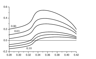
Figure 8: Transfer free energy ($\Delta g^{*}/\eta$) as a function of temperature ($T/\eta$) for a single monomer at liquid-vapor coexistence, for $\epsilon_{\mathsf{ws}}/\eta=0,0.03,0.05,0.08,0.09,0.10$. Other parameter values: $\epsilon_{\mathsf{ww}}/\eta=0.25$, $w=20$, $c_{\mathsf{w}}=0.5$, $\epsilon_{\mathsf{ss}}=0$, $c_{\mathsf{s}}=0$.

As a general trend, the curves are shifted towards lower energy values, upon increasing $\epsilon_{\mathsf{ws}}$, while the maximum becomes broader. Such behavior qualitatively accounts for progressive hindering of the collapsed state observed in the polymer model. Nevertheless, we find it remarkable that, from the solvation free energy alone, one would not at all expect the previously described variety of behaviors. In our opinion, this is a striking evidence of the fact that inverse swelling cannot be satisfactorily modeled by effective interaction potentials, meant to take into account a temperature-dependent “quality of the solvent”, but it is rather to be ascribed to a subtler interplay between polymer and water degrees of freedom.

V Conclusions

In this paper, we have proposed and investigated a lattice model of a linear hydrophobic homopolymer in aqueous solution. As far as water is concerned, the model is a simplified version of a model proposed by Roberts and Debenedetti Roberts and Debenedetti (1996), in which we have removed distinction between donors and acceptors, which is generally believed not to play a crucial role in the thermodynamics of hydrogen bonding Southall et al. (2002). With respect to other simplified model addressed to study the same kind of systems and phenomenology, the main new ingredient of the present work is that we have extended a previously studied model of water and aqueous solutions to the case in which the solute is a polymer, without other ad-hoc assumptions.

We observe the inverse swelling phenomenon, i.e., a transition from a collapsed to a swollen state upon decreasing temperature. For an ideally inert (hydrophobic) polymer, such transition is first order, and occurs at very low temperatures, where we expect that liquid water is unstable. In this respect, our model results can be viewed just as an extrapolation. Nevertheless, the transition can be moved into the temperature region of liquid water by an attractive water-monomer interaction. In these conditions, inverse swelling is no longer purely first order, but occurs via a discontinuous transition to a moderately collapsed phase, followed by a $\Theta$-like transition to a completely swollen state. The latter transition likely stays in the unobservable region, so that we expect that only first order swelling could be observed. Upon increasing pressure, the first order transition temperature increases, the transition is smoothed, and eventually disappears at high pressure values. Let us briefly discuss the relevance of such findings to experimental results.

First of all, the typical system in which the inverse swelling phenomenon can be observed is an aqueous solution of a thermoreversible homopolymer, such as poly-N-isopropylacrylamide (PNIPAM) Tiktopulo et al. (1995); Wu and Zhou (1996); Wu and Wang (1998). It is interesting to notice that, for PNIPAM, inverse swelling occurs actually via a first order transition at a temperature close to $27^{\circ}\,\mathrm{C}$, at ordinary pressures. In the framework of our model, a similar behavior can be reproduced, as previously mentioned, only in the presence of a water-segment attractive interaction. For PNIPAM, the existence of such attraction can be justified by the fact that the monomeric unit (NIPAM) contains in the side chain a polar (hydrophilic) peptide group, beside ten non-polar (hydrophobic) hydrogens (the structure is reported for instance in Ref. Tiktopulo et al., 1995). It is noteworthy that the assumption of such kind of interaction had to be made as well in a previous phenomenological treatment of the inverse swelling phenomenon for PNIPAM Bruscolini et al. (2002). In the cited article, the solvation free energy for NIPAM was assumed as an effective temperature-dependent interaction with water, and, as a consequence, inverse swelling turned out to be a $\Theta$-like point, i.e., a continuous transition. Conversely, from our investigation it clearly turns out that the information contained in the solvation free energy is insufficient to discriminate the type of transition.

A purely hydrophobic short polymer chain in water has been recently investigated in great detail, by means of molecular dynamics simulations Paschek et al. (2005). Beside several structural results, it has turned out that inverse swelling cannot be observed at ordinary pressures, but only at very high pressures. The transition is abrupt enough to suppose that it becomes discontinuous in the thermodynamic limit, and the transition temperature increases with pressure. These results qualitatively agree with our findings, although for our model the effect of pressure is not sufficient to move the transition in the observable region, for the completely inert polymer.

We have mentioned in the Introduction that some interest on the inverse swelling phenomenon has been attracted by the fact that globular proteins undergo a somehow similar phenomenon, known as cold unfolding. Our model is definitely too simple to describe the physics of proteins, first of all since a protein is a heteropolymer, in which the monomeric units have different degrees of affinity with water. Nonetheless, some interesting analogies exist. In most cases, the cold unfolding transition of proteins can be observed in the temperature regime of stable liquid water, in the presence of denaturants (urea) Privalov (1990), or by applying high pressures (pressure denaturation) Panick et al. (1999); Herberhold and Winter (2002). Extrapolations to zero denaturant concentration, or to ambient pressure, suggest a transition temperature below the freezing temperature of water. Both effects seem to be somehow consistent with our results. On the one hand, a denaturant could be roughly viewed as something which on average makes the protein more hydrophilic, i.e., a water-segment attractive interaction. On the other hand, we have observed that pressure tends to increase the transition temperature, although this effect is relatively weak.

Let us finally recall that the results presented here have been obtained by an approximate technique, i.e., a generalized first-order approximation. Such kind of calculation requires quite a negligible computational effort, but usually provides qualitatively reliable results. In particular, the accuracy of the approximation has been previously verified, by a comparison with Monte Carlo simulations, both for the pure water model Pretti and Buzano (2004) and, independently, for an ordinary self-avoiding walk model with stiffness Pretti (2002). Nevertheless, a similar test for the full model would be welcome, but this goes beyond the scope of the present paper, and is left to future work.

*

Appendix A Equilibrium free energy

Hereafter, we justify the formula employed in the text to evaluate the equilibrium (grand-canonical) free energy density. It is known that the exact solution of a Husimi lattice can be obtained also in a variational approach, as a minimum of a generalized Bethe free energy Pretti (2003). Eq. (9) could be written in principle from the general free energy formula reported in Ref. Pretti, 2003, but this formula has been proved only for the case of scalar configuration variables. Here, although with some tricks we can label configurations with scalar quantities, polymer configurations actually behaves as vector variables, which is revealed by the presence of “primed” configurations in Eqs. (5) and (6). Therefore, we have to extend the proof, restarting from the variational Bethe free energy. For our particular system, in the homogeneity hypothesis, the Bethe free energy per site can be written as

$$\omega/T=\left\langle\mathcal{H}_{ijkl}/T+\ln P_{ijkl}\right\rangle-3\left\langle\ln p_{i}\right\rangle,$$ (16)

where $\langle\cdot\rangle$ denotes an ensemble average over configuration variables, and $P_{ijkl}$ is the tetrahedron probability distribution. Let us notice that the previous formula holds for a generic free energy density, not necessarily the grand-canonical one. The tetrahedron probability distribution can be written as a function of the partial partition functions in the following form

$$P_{ijkl}=Z^{-1}e^{-\mathcal{H}_{ijkl}/T}\prod_{\xi=\prime}^{\prime\prime\prime}q_{i^{\xi}}q_{j^{\xi}}q_{k^{\xi}}q_{l^{\xi}},$$ (17)

which results by considering the operation of attaching $3$ branches to each site of the given tetrahedron. The normalization constant is

$$Z=\sum_{i=0}^{8}w_{i}\sum_{j=0}^{8}w_{j}\sum_{k=0}^{8}w_{k}\sum_{l=0}^{8}w_{l}e^{-\mathcal{H}_{ijkl}/T}\prod_{\xi=\prime}^{\prime\prime\prime}q_{i^{\xi}}q_{j^{\xi}}q_{k^{\xi}}q_{l^{\xi}}.$$ (18)

Replacing Eqs. (17) and (6) into (16), and taking into account the linearity of the average operation, one obtains by simple algebra

$$\omega/T=-\ln Z+3\ln z+\Phi,$$ (19)

where

$$\Phi=\sum_{\xi=\prime}^{\prime\prime\prime}\left\langle\ln\frac{q_{i^{\xi}}}{q_{i}}\right\rangle=\sum_{\xi=\prime}^{\prime\prime\prime}\sum_{i=0}^{8}w_{i}p_{i}\left(\ln q_{i^{\xi}}-\ln q_{i}\right).$$ (20)

Expanding the sum, and inserting the multiplicity values $w_{i}$ reported in Table 1, one can write

$$\Phi = 3\left(p_{6}-p_{4}\right)\ln q_{4}+3\left(p_{4}-p_{6}\right)\ln q_{6}$$

$$+12\left(p_{7}+p_{8}-2p_{5}\right)\ln q_{5}$$

$$+6\left(2p_{5}+p_{8}-3p_{7}\right)\ln q_{7}+6\left(2p_{5}+p_{7}-3p_{8}\right)\ln q_{8},$$

where the terms associated to configurations $i=0,1,2,3$ (empty site or water) disappear, because in this case $i=i^{\prime}=i^{\prime\prime}=i^{\prime\prime\prime}$ holds (see Table 1). As mentioned in the text, one can observe that $p_{4}=p_{6}$ and $p_{5}=p_{7}=p_{8}$, whence $\Phi=0$. Moreover, making use of Eqs. (18), (5), and (7), it is possible to show that

$$Z=yz,$$ (22)

where $y$ is the normalization constant of the recursion equation (5), which has to be computed at each iteration, and $z$ is given by Eq. (7). Replacing the previous equation into Eq. (19) with $\Phi=0$, one finally obtains Eq. (9), which we aimed to prove.