Continuous phase transition of a fully frustrated XY model in three dimensions

Abstract

We have used Monte Carlo simulations, combined with finite-size scaling and two different real-space renormalization group approaches, to study a fully frustrated three-dimensional XY model on a simple cubic lattice. This model corresponds to a lattice of Josephson-coupled superconducting grains in an applied magnetic field ${\bf H}=(\Phi_{0}/a^{2})(1/2,1/2,1/2)$. We find that the model has a continuous phase transition with critical temperature $T_{c}=0.681J/k_{\mathrm{B}}$, where $J$ is the XY coupling constant, and critical exponents $\alpha/\nu=0.87\pm 0.01$, $v/\nu=0.82\pm 0.01$, and $\nu=0.72\pm 0.07$, where $\alpha$, $v$, and $\nu$ describe the critical behavior of the specific heat, helicity modulus, and correlation length. We briefly compare our results with other studies of this model, and with a mean-field approximation.

I Introduction

The classical XY model has been widely used for decades as a model for phase transitions in materials with interacting spins. The dimensionality $n$ of the spins ($n=2$ for the XY model) is independent of the lattice dimensionality $d$, which can be either $2$ or $3$ for physically relevant systems. The $d=2$ XY model undergoes the well-known Kosterlitz-Thouless (KT) transition kt , characterized by an unbinding of vortex-antivortex pairs at the KT transition temperature $T_{\mathrm{KT}}$. The KT transition is a continuous phase transition, but with unique critical properties kt . The $d=3$ XY model exhibits a more conventional phase transition with well-known critical exponents li1 ; gottlob2 . It is thought to describe many ferromagnetic materials with two-component spins. In addition, it describes phase transitions in which the “spins” actually represent the phases of a complex order parameter, such as the $\lambda$ transition in He⁴ and superconductor-to-normal phase transition at zero applied magnetic field.

The frustrated classical XY model, in either $d=2$ or $d=3$, has a much wider range of phase diagrams than does the unfrustrated case just mentioned. In this model, the coupling between spins is such that the ground state of the system cannot minimize all the bond energies simultaneously. Interest in this model was greatly increased when it was realized that this model described real systems, such as Josephson junction arrays in an applied magnetic field. The first demonstration that the fully frustrated XY model undergoes a continuous phase transition in $d=2$ was given by Teitel and Jayaprakash teitel1 , using Monte Carlo (MC) techniques. This work was later extended to other values of the so-called frustration parameter $f$ teitel2 , leading to an extensive literature on two-dimensional (2D) frustrated XY model on various lattices and at different values of $f$ cataudella ; gottlob ; dukovski .

The $d=3$ frustrated XY model has also been studied extensively, in part because it is believed to describe flux line lattice (FLL) melting nelson1 under an applied magnetic field in high-T_c superconductors. Hetzel et al. hetzel used a uniformly frustrated 3D XY model on a stacked triangular lattice to study the melting of an unpinned Abrikosov lattice in a type-II superconductor. They showed convincingly that this melting transition is first order, rather than continuous — a prediction subsequently confirmed by experiment. Earlier work on a frustrated XY model on a simple cubic lattice, with magnetic field parallel to one of the lattice axes shih1 found a continuous phase transition. Li and Teitel li2 ; li3 used a uniformly frustrated XY model similar to that of Ref. hetzel to calculate the properties of the vortex line liquid which appears above the melting temperature, and to investigate the possibility of a further phase transition between an entangled and a disentangled vortex line liquid above the FLL melting transition. Chen and Teitel chen later extended this work to the more realistic case of uniaxially anisotropic couplings; they suggested that there was another phase transition temperature $T_{cz}$ above the FLL melting temperature $T_{m}$, where superconducting coherence parallel to the applied magnetic field would vanish. Chin et al. chin have, however, suggested that this apparent existence of a transition to a disentangled vortex liquid is a result of finite system sizes and simulation times. More recently, the uniformly frustrated 3D XY model was studied by Monte Carlo methods on a simple cubic lattice with a magnetic field parallel to the $[111]$ direction hwang . For this choice of field direction, the simple cubic lattice behaves as a stack of 2D triangular lattices with $ABCABC\cdots$ stacking. It was found that this system, similar to that studied in Ref. hetzel , exhibits a clear first-order FLL melting transition. Nguyen and Sudbø nguyen1 considered a uniformly frustrated anisotropic Villain model (an approximation to the uniformly frustrated XY model) to study the phase diagram of a uniaxially anisotropic high-T_c superconductor as a function of the applied magnetic field and temperature. They found two phase transitions: the lower-temperature one is FLL melting, while that at higher temperature involves the destruction of the phase coherence in the direction of the applied magnetic field.

In this paper, we study phase transitions in the fully frustrated XY model in $d=3$, using primarily MC simulations. This model is of interest, in part, because it may be relevant to FLL melting in the high-T_c materials. In addition, because of great advances in microfabrication techniques, it is now possible to make microscale or nanoscale arrays of Josephson superconducting grains in three dimensions. Such an array should, in a suitable applied magnetic field, be describable by a frustrated XY model, at least to a first approximation. It has also recently been suggested that a fully frustrated XY model might also be realized by an assembly of cold atoms on a suitably constructed optical lattice polini .

The fully frustrated XY model is characterized by the frustration vector ${\bf f}=(1/2,1/2,1/2)$, as further defined below. Such a model has been previously studied by Diep et al. diep , who found that, in contrast to the ${\bf f}=(1/3,1/3,1/3)$ case studied in Ref. hwang , there was a continuous phase transition. We extend the work of Ref. diep by calculating the critical behavior of the helicity modulus, equivalent to the spin-wave stiffness constant (or to the superfluid density in a superconductor). We also carry out a more extensive finite-size scaling analysis than done by those workers, thus obtaining more accurate information about the critical behavior. Our results do, however, confirm that the phase transition is continuous, not first order.

The remainder of this paper is organized as follows. In Sec. II, we present the formalism for calculating the thermodynamic properties and the critical exponents of our model. In Sec. III, we give the results of our Monte Carlo calculations, finite-size scaling methods, and renormalization group methods. Section IV presents a summary and discussions.

II Formalism

We now describe the model Hamiltonian on which our calculations are carried out. For convenience, we present this Hamiltonian as it applies to a simple cubic lattice of superconducting grains in the presence of an applied external magnetic field ${\bf H}$, though the model is not limited to this application, of course. Then the frustrated XY model in $d=3$ is described by the Hamiltonian

$$\mathcal{H}=-\sum_{\langle ij\rangle}J_{ij}\cos(\phi_{i}-\phi_{j}-A_{ij}).$$ (1)

Here $\phi_{i}$ is the phase of the superconducting order parameter on the $i$th site, $A_{ij}=(2\pi/\Phi_{0})\int_{i}^{j}{\bf A}\cdot d{\bf l}$, $\Phi_{0}=hc/2e$ is the flux quantum, ${\bf A}$ is the vector potential, $J_{ij}$ is the coupling constant between the $i$th site and $j$th site, and $\langle ij\rangle$ represents a sum over all distinct pairs of nearest-neighbor sites on a simple cubic lattice. We assume a constant coupling between each nearest-neighbor pair of sites, so $J_{ij}=J$ and $J>0$; we neglect the possible dependence of $J$ on the applied magnetic field ${\bf H}$ and the temperature $T$. We also assume weak screening as in Ref. hwang . Thus, the local magnetic field ${\bf B}$ is approximated by the applied magnetic field ${\bf H}$.

The $x$ component of the frustration vector ${\bf f}=(f_{x},f_{y},f_{z})$ is defined by

$$\sum_{p}{{}^{(x)}}A_{ij}=2\pi f_{x},$$ (2)

where the sum is taken along the sides of a plaquette on the $yz$ plane of the lattice; analogous definitions hold for $f_{y}$ and $f_{z}$. If the simple cubic lattice has lattice constant $a$, $f_{i}=B_{i}a^{2}/\Phi_{0}$ represents the flux through a single plaquette perpendicular to the $i$th axis, in units of one flux quantum.

One can also define the vortex number (or vorticity) of each square plaquette. For example, the vorticity of a plaquette lying in the $yz$ plane is defined by

$$n_{x}=f_{x}+\frac{1}{2\pi}\sum_{p}{{}^{(x)}}(\phi_{i}-\phi_{j}-A_{ij}),$$ (3)

where the sum runs counterclockwise around the perimeter of the plaquette, viewed from the positive $x$ direction, and the phase differences are chosen so that $0\leq\phi_{i}<2\pi$. $n_{y}$ and $n_{z}$ are defined analogously.

In order to study possible phase transitions within this model, we have calculated several quantities. One of these is the specific heat $C_{V}$ per site, given by

$$C_{V}=\frac{\langle\mathcal{H}^{2}\rangle-\langle\mathcal{H}\rangle^{2}}{Nk_{\mathrm{B}}T^{2}},$$ (4)

where $N$ is the total number of sites in the lattice, $\mathcal{H}$ is the Hamiltonian in Eq. (1), and $\langle\cdots\rangle$ denotes an average within the canonical ensemble. A first-order phase transition is generally indicated by a $\delta$-function-like anomaly in $C_{V}$, while a continuous phase transition is signaled by lattice-size-dependent divergence in the $C_{V}$.

To study the vortex lattice melting, we calculate a suitable vorticity density-density correlation function. Specifically, we first introduce the Fourier transform of the vorticity density $n_{i}({\bf k})=\sum_{\bf R}n_{i}({\bf R})\exp(i{\bf k}\cdot{\bf R})$, where $n_{i}({\bf R})$ represents the vorticity of a plaquette centered at ${\bf R}$ and oriented perpendicular to the $i$th axis. We then calculate some of the correlation functions

$$g_{ij}({\bf r})=\frac{1}{N^{2}f_{i}f_{j}}\sum_{{\bf R},{\bf R}^{\prime}}{{}^{\prime}}\langle n_{i}({\bf R})n_{j}({\bf R}^{\prime})\rangle,$$ (5)

where the sum is carried out over all ${\bf R}$ and ${\bf R}^{\prime}$ such that ${\bf R}^{\prime}-{\bf R}={\bf r}$. In our actual simulations, we use periodic boundary conditions in all three directions. In practice, it is more convenient to compute the Fourier transform of $g_{ij}({\bf r})$. This Fourier transform is known as the vortex structure factor, and is given by $S_{ij}({\bf k})=\sum_{\bf r}g_{ij}({\bf r})e^{i{\bf k}\cdot{\bf r}}$. Because of the periodic boundary conditions, $S_{ij}({\bf k})$ is defined only for ${\bf k}=[2\pi/(N_{x}a)](m_{1},m_{2},m_{3})$, where $m_{i}$ are integers, and the computational cell is assumed to contain $N=N_{x}^{3}$ sites. We obtain $g_{ij}({\bf r})$ by first computing $S_{ij}({\bf k})$ and then Fourier-transforming back into real space.

The phase transition in this model is best characterized by the helicity modulus tensor $\gamma_{\alpha\beta}$ fisher . $\gamma_{\alpha\beta}$ measures the stiffness of the phase $\phi$ against an external twist. It is defined as the second derivative of the free energy with respect to an infinitesimal phase twist ohta

$$\gamma_{\alpha\beta}=\frac{1}{N}\left.\frac{\partial^{2}F}{\partial\delta_{\alpha}\partial\delta_{\beta}}\right|_{\delta=0}.$$ (6)

$\gamma_{\alpha\beta}$ is conveniently calculated by adding a fictitious vector potential ${\bf A}^{\prime}$ to the Hamiltonian in Eq. (1), as

$$\gamma_{\alpha\beta}=\frac{1}{N}\left.\frac{\partial^{2}F}{\partial A_{i}^{\prime}\partial A_{j}^{\prime}}\right|_{{\bf A}^{\prime}=0},$$ (7)

in the presence of periodic boundary conditions on the phases. The resulting diagonal components are readily evaluated, with the result

$$\gamma_{\alpha\alpha} = \frac{1}{N}\left\langle\sum_{\langle ij\rangle}J_{ij}\cos(\phi_{i}-\phi_{j}-A_{ij})(\mbox{\^{e}}_{ij}\cdot\mbox{\^{e}}_{\alpha})^{2}\right\rangle$$ (8)

$$- \frac{1}{Nk_{B}T}\left\langle\left[\sum_{\langle ij\rangle}J_{ij}\sin(\phi_{i}-\phi_{j}-A_{ij})(\mbox{\^{e}}_{ij}\cdot\mbox{\^{e}}_{\alpha})\right]^{2}\right\rangle$$

$$+ \frac{1}{Nk_{B}T}\left\langle\sum_{\langle ij\rangle}J_{ij}\sin(\phi_{i}-\phi_{j}-A_{ij})(\mbox{\^{e}}_{ij}\cdot\mbox{\^{e}}_{\alpha})\right\rangle^{2}.$$

Here $\mbox{\^{e}}_{ij}$ is the unit vector from the $i$th site to the $j$th site, and $\mbox{\^{e}}_{\alpha}$ is the unit vector in the $\alpha$ direction. Since the helicity modulus $\gamma_{\alpha\alpha}$ is proportional to the $\alpha$ component of the superfluid density, it follows that when $\gamma_{\alpha\alpha}>0$, there is nonzero phase coherence in the $\alpha$ direction, and when $\gamma_{\alpha\alpha}\rightarrow 0$, the phase coherence is lost. Therefore, the superconductor-to-normal phase transition occurs at the temperature at which $\gamma_{\alpha\alpha}\rightarrow 0$.

The correlation time $\tau$ is a measure of how long it takes for the system to lose its memory of its previous state. $\tau$ can be obtained by calculating a time-displaced autocorrelation function newman4 . The time-displaced autocorrelation function $\chi_{E}(t)$ of the energy, for example, is defined by

$$\chi_{E}(t) = \int[E(t^{\prime})-\langle E\rangle][E(t^{\prime}+t)-\langle E\rangle]\mathrm{d}t^{\prime}$$ (9)

$$= \int[E(t^{\prime})E(t^{\prime}+t)-\langle E\rangle^{2}]\mathrm{d}t^{\prime},$$

where $t$ and $t^{\prime}$ are two different Monte Carlo “times.” Since Monte Carlo simulations involve fictitious dynamics, these times are not related in any obvious way to a physical time. However, the length of the Monte Carlo time does give a measure of the persistence of various MC states in time.

Equation (9) can be expressed more conveniently when we have a set of measurements of the energy $E(t)$ from $t=0$ (after equilibration) up to some maximum time $t_{\max}$. In this case, Eq. (9) becomes

$$\chi_{E}(t) = \frac{1}{t_{\max}-t}\sum_{t^{\prime}=0}^{t_{\max}-t}E(t^{\prime})E(t^{\prime}+t)$$ (10)

$$- \frac{1}{(t_{\max}-t)^{2}}\sum_{t^{\prime}=0}^{t_{\max}-t}E(t^{\prime})\sum_{t^{\prime}=0}^{t_{\max}-t}E(t^{\prime}+t).$$

Since the autocorrelation function is expected to fall off exponentially at long times as

$$\chi_{E}(t)\sim e^{-t/\tau},$$ (11)

the correlation time $\tau$ can be calculated from

$$\int_{0}^{\infty}\frac{\chi_{E}(t)}{\chi_{E}(0)}\mathrm{d}t=\int_{0}^{\infty}e^{-t/\tau}\mathrm{d}t=\tau.$$ (12)

This expression for $\tau$ is also called integrated correlation time. MC “measurements” will be statistically independent only if they are separated by intervals of $\sim 2\tau$ or more. In addition, the correlation time $\tau$ is related to the dynamic exponent $z$ by

$$\tau\sim\xi^{z}\sim L^{z},$$ (13)

where $\xi$ is the correlation length (equal to $L$ at the $T_{c}(L)$). The dynamic exponent measures the extent of the critical slowing down. The smaller $z$ is, the more accurate are the numerical measurements.

If there is a continuous phase transition, various quantities should exhibit singular behavior near the transition temperature $T_{c}$. If we define a reduced temperature by

$$t=\frac{T-T_{c}}{T_{c}},$$ (14)

then in the thermodynamic limit the correlation length $\xi$, the specific heat per site $C_{V}$, and the helicity modulus $\gamma$ near $T_{c}$ are expected to vary as

$$\xi \sim |t|^{-\nu},$$ (15)

$$C_{V} \sim |t|^{-\alpha},$$ (16)

$$\gamma \sim |t|^{v},$$ (17)

where $\nu$, $\alpha$, and $v$ are critical exponents. If $T_{c}$ is known, the simulation data can be fitted to the expected asymptotic form to obtain values of the critical exponents. But since $T_{c}$ is typically not known in advance, it is usually more accurate to use a different method. One such method is finite-size scaling, which extracts values for the critical exponents by investigating how measurements depend on the size $L$ of the system newman2 . This procedure is carried out by expressing a quantity of interest in terms of the correlation length and then introducing a new dimensionless function, known as a scaling function. For example, $C_{V}$ and $\gamma$ are expressed as

$$C_{V}(L,t) = L^{\alpha/\nu}\tilde{C_{V}}(L^{1/\nu}t),$$ (18)

$$\gamma(L,t) = L^{-v/\nu}\tilde{\gamma}(L^{1/\nu}t),$$ (19)

where $L=N_{x}a$ is the linear system dimension. Since the scaling functions $\tilde{{C}_{V}}$ and $\tilde{\gamma}$ should depend on a single variable, we can make all the data for each system size $L$ fall on the same curve by appropriately adjusting the values of the critical exponents and $T_{c}$. When this happens, we assume that we have the correct values for these quantities.

Another method is the phenomenological renormalization group (PRG) barber ; nightingale ; li1 . To calculate the critical behavior of $\gamma$, for example, we consider two different system sizes $L$ and $L^{\prime}$ and introduce the ratio

$$P_{\gamma}(L,L^{\prime},t)\equiv\frac{\gamma(L,t)}{\gamma(L^{\prime},t)}.$$ (20)

From Eq. (19) this ratio becomes $P_{\gamma}=(L/L^{\prime})^{-v/\nu}$ when $t=0$. Therefore, if one plots two different curves of $P_{\gamma}(L,L^{\prime},t)$ versus $t$ with the same ratio of $L/L^{\prime}$, the temperature at which they intersect is $T_{c}$, and the value of $P_{\gamma}$ at that temperature yields the ratio $v/\nu$.

The critical temperature $T_{c}$, or its inverse value $K_{c}=J/(k_{\mathrm{B}}T_{c})$, and the critical exponent $\nu$ can also be determined from Binder’s fourth-order cumulant $U_{L}$ binder defined by

$$U_{L}=1-\frac{\langle s^{4}\rangle}{3\langle s^{2}\rangle^{2}},$$ (21)

where $s=(1/N)\sqrt{(\sum_{i}^{N}\cos\phi_{i})^{2}+(\sum_{i}^{N}\sin\phi_{i})^{2}}$. The scaling form for the Binder’s cumulant is $U_{L}=\tilde{U}(L^{1/\nu}t)$, without any prefactor. Hence, $U_{L}$ can be Taylor expanded about $T_{c}$ as

$$U_{L} = U_{0}+U_{1}L^{1/\nu}\left(1-\frac{T}{T_{c}}\right)+\cdots$$ (22)

$$= U_{0}+U_{1}L^{1/\nu}\left(1-\frac{K_{c}}{K}\right)+\cdots.$$

If we plot $U_{L}$ for several values of $L$ as a function of temperature or its inverse value, they will intersect at the critical temperature $T_{c}$. To obtain the exponent $\nu$, we can calculate $(\mathrm{d}U_{L}/\mathrm{d}K)_{K=K_{c}}$, where $K=J/(k_{\mathrm{B}}T)$. From Eq. (22), we find that

$$\left.\frac{\mathrm{d}U_{L}}{\mathrm{d}K}\right|_{K_{c}}=\frac{U_{1}}{K_{c}}L^{1/\nu}.$$ (23)

Hence, the ratio of the two slopes for different values of $L$ gives $\nu$.

III Monte Carlo Calculations

To carry out our Monte Carlo calculations, we used the standard Metropolis algorithm with periodic boundary conditions in all three directions. We started with a random phase configuration at temperature $T=1.0J/k_{\mathrm{B}}$, then cooled down to $T=0.4J/k_{\mathrm{B}}$ in steps of $0.01J/k_{\mathrm{B}}$, except near $T_{c}$, where we decreased the temperature in steps of $0.005J/k_{\mathrm{B}}$. At each $T$, we took 50000 Monte Carlo steps per site through the entire lattice for equilibration, and then calculated the expectation values of the quantities of interest by averaging over an additional 20000 MC steps. We also used the final configuration of the previous $T$ as the starting one of the current $T$. Near $T_{c}$, the system undergoes critical slowing down; so we increased the number of MC steps up to $5\times 10^{5}$ for equilibration and $2\times 10^{5}$ for averaging.

Instead of considering continuous angles between $0$ and $2\pi$ for the phases $\phi_{i}$ of the order parameter on each site, we used the 360-state clock model, which allows angles of $0^{\circ}$, $1^{\circ}$, $2^{\circ}$,…, $359^{\circ}$. This simplification should have no effect on our results, since it is known that there is no distinction between the continuum and the discrete results for the $n$-state clock model when $n>20$ thijssen .

To calculate the phase factors $A_{ij}$, we use the gauge ${\bf A}=(\Phi_{0}/a^{2})(f_{y}z\hat{x}+f_{z}x\hat{y}+f_{x}y\hat{z})$, where the frustration is ${\bf f}=f_{x}\hat{x}+f_{y}\hat{y}+f_{z}\hat{z}$. Thus, for example, the phase factors $A_{ij}^{(z)}$ arising from the field component parallel to $z$ all vanish except for bonds in the $y$ direction; for these bonds, and $x=na$, $A_{ij}^{(z)}$ is given by

$$A_{ij}^{(z)}=2\pi nf_{z}.$$ (24)

The phase factors $A_{ij}^{(x)}$ and $A_{ij}^{(y)}$ are given by analogous expressions. For ${\bf f}=(1/2,1/2,1/2)$ and periodic boundary conditions in all three directions, all the phase factors are equal to either $0$ or $\pi$, and thus all the couplings are of the form $\pm J\cos(\phi_{i}-\phi_{j})$. This choice of gauge automatically satisfies the condition given in Eq. (2).

We turn now to our numerical results. The values of the correlation time $\tau$ for several lattice sizes are given in Table I, at the estimated transition temperature $T_{c}(L)$ for the fully frustrated XY model [${\bf f}=(1/2,1/2,1/2)$] of size $L=N_{x}a$. $\tau$ clearly increases monotonically with increasing lattice size. From the fits to data in Fig. 1, we get the dynamic exponent $z=2.23\pm 0.14$ in our system.

The internal energy per site $U\equiv E/N$, expressed in units of the coupling constant $J$, is shown in Fig. 2. It is quite size-dependent for $L<10$ but quickly converges for $L>10$. The sharp drop in $U$ near $T=0.7J/k_{\mathrm{B}}$ suggests but obviously does not prove the occurrence of a phase transition near that temperature.

The calculated specific heat per site $C_{V}$ is shown in Fig. 3. There is a clear peak near $T\sim 0.7J/k_{\mathrm{B}}$ which becomes sharper with increasing $L$, suggesting a continuous phase transition. This behavior is similar to that of the 2D fully frustrated XY model as in Ref. teitel1 and that of the ordered simple cubic lattice with ${\bf f}=(0,0,1/2)$, as in Ref. shih1 . As in those two examples, the finite magnitude of $C_{V}$ at its peak is a result of the finite system size; otherwise, $C_{V}$ would diverge at $T_{c}$ in the infinite system.

Next, we turn to the behavior of the helicity modulus tensor. Since $\gamma_{xx}=\gamma_{yy}=\gamma_{zz}$ for this isotropic system, we calculated the average $\gamma=(\gamma_{xx}+\gamma_{yy}+\gamma_{zz})/3$ in order to improve the statistics. $\gamma(T)$ increases with decreasing $T$, and shows a fairly clear drop to near zero near $T=0.7J/k_{\mathrm{B}}$ when $L>10$, as can be seen in Fig. 4. For $L=10$ or smaller, $\gamma(T)$ shows a broad transition region. A more accurate value for $T_{c}$ will be given further below.

To estimate the statistical errors in our calculation of $\gamma(T)$, we used the jackknife method newman3 , which is carried out as follows. For each $T$, we made $n$ independent numerical measurements of $\gamma(T)$, with measurements separated by at least two correlation times. From these $n$ measurements, we calculated a value $\gamma(T)$ for the helicity modulus. Next, we removed the first measurement from this set of $n$ measurements to calculate the helicity modulus $\gamma_{1}$ with the remaining $n-1$ measurements. To calculate $\gamma_{2}$ we restored the first measurement to the set and removed the second measurement, and so on. Thus, $\gamma_{i}$ is calculated with the $i$th measurement removed from the set. The error estimate for $\gamma$ is given by

$$\sigma_{\gamma}=\sqrt{\sum_{i=1}^{n}(\gamma_{i}-\gamma)^{2}}.$$ (25)

The error bars from this method are shown in Fig. 4, but they are smaller than the symbol sizes.

In Fig. 5, we show the evolution of the internal energy per site $U$ as a function of MC time at the transition temperature $T_{c}=0.681J/k_{\mathrm{B}}$ for a lattice size $12\times 12\times 12$. The three intensity plots for each $a$ and $b$ show the density-density correlation functions $g_{zz}(x,y,L_{z}/2)$, $g_{xx}(L_{x}/2,y,z)$, and $g_{yy}(x,L_{y}/2,z)$ (denoted by $xy$, $yz$, and $zx$, respectively) of the vortices at two different times as indicated in the energy evolution curve. Each intensity plot is an average of one correlation time $\tau=148$ MC steps per site through the entire lattice. The two times correspond to energies slightly below and slightly above the average value and they are separated by a very large MC time. In contrast to the results of Ref. hwang , there is no indication of a vortex lattice phase in these plots; instead, both seem to show vortex liquid phases (although there are partial latticelike formations, especially on the $zx$ plane in window $a$). This behavior suggests (as does the diverging specific heat peak in Fig. 3) that the phase transition at ${\bf f}=(1/2,1/2,1/2)$ is continuous, rather than first order as at ${\bf f}=(1/3,1/3,1/3)$. However, at very low temperatures ($T=0.01J/k_{\mathrm{B}}$), the correlation functions show a clearer indication of an ordered phase, as shown in Fig. 6. Specifically, we see evidence of a checkerboard lattice in all three directions, but especially in the $yz$ windows.

This ordering is clearer if we look at the vortex structure factor $S_{zz}({\bf k})$ of the lattice. Figure 7 shows this structure factor for ${\bf k}$ parallel to the magnetic field, at several temperatures, including the two shown in Figs. 5 and 6. Here $k_{\|}=|{\bf k}|$ and ${\bf k}=[2\pi/(N_{x}a)](m,m,m)$, where $m=0$, $1$,…, $N_{x}-1$. At low temperatures, the vortex structure factors at $k_{\|}=\sqrt{3}\pi/a$ are nonzero, but they do not increase monotonically with decreasing temperature. Instead, they increase down to $T=0.30J/k_{\mathrm{B}}$, then decrease down to $T=0.01J/k_{\mathrm{B}}$. We believe that this behavior may represent some kind of “polycrystalline” domain structure of the vortex at low temperatures. As shown below, the system has several eigenmodes, and the exact admixture of these eigenmodes may change as the temperature varies. The insets to Fig. 7 are the vortex density-density correlation functions $g_{zz}(x,y,L_{z}/2)$ at two different temperatures $T=0.30J/k_{\mathrm{B}}$ and $T=0.681J/k_{\mathrm{B}}$. We can see a clear checkerboard pattern at $T=0.30J/k_{\mathrm{B}}$. The vortex structure factor appears to go to zero near the same temperature as $T_{c}$ where the helicity modulus vanishes, although we did not collect enough numerical data to determine the temperature dependence of the structure factor peak near $T_{c}$. This point is discussed further below.

In Fig. 8, we show the probability distribution $P(U)$ of the internal energy per site $U$ for several lattice sizes at $T_{c}$. For each lattice size, we see only a single peak, which sharpens with increasing lattice size. This result is also in contrast to that of Ref. hwang , where the single peak splits into two peaks as the lattice size increases. This persistent single-peak behavior suggests a continuous phase transition, in contrast to the first-order phase transition found in Ref. hwang .

The data shown in Fig. 3 can be used in a standard way to obtain an estimate of the critical exponent ratio $\alpha/\nu$. From Eqs. (15) and (16), the maximum value of $C_{V}$ for a lattice of edge $L$ is

$$C_{V}^{\max}\sim\xi^{\alpha/\nu}\sim L^{\alpha/\nu}.$$ (26)

In Fig. 9, we plot $\log C_{V}^{\max}$ versus $\log L$ at $T=T_{c}$. The data is well described by a straight line. The slope of this fitted straight line gives $\alpha/\nu=0.87\pm 0.01$. The present result is in contrast to the linear relation between $C_{V}$ and $\log L$, corresponding to $\alpha=0$ (logarithmic divergence) seen in the fully frustrated 2D XY model as in Ref. teitel1 .

As we did for the specific heat $C_{V}$, we see from Eqs. (15) and (17), or just from Eq. (19), that the helicity modulus $\gamma$ depends on the lattice size $L$ as

$$\gamma\sim\xi^{-v/\nu}\sim L^{-v/\nu}.$$ (27)

In Fig. 10, we plot $\log\gamma$ versus $\log L$ at two different temperatures $T=0.681J/k_{\mathrm{B}}$ and $T=0.682J/k_{\mathrm{B}}$. From the fits to the data, we get $v/\nu=0.79\pm 0.02$ at $T=0.681J/k_{\mathrm{B}}$ and $v/\nu=0.83\pm 0.02$ at $T=0.682J/k_{\mathrm{B}}$. The error bars from the jackknife method are also shown, but they are smaller than the symbol sizes. The value of $v/\nu$ is very sensitive to small changes in the assumed $T_{c}$. So we need a more reliable method to calculate $v/\nu$. In Fig. 11, we show the results of a PRG study of the helicity modulus $\gamma(L,t)$. As described near Eq. (20), we plot $P_{\gamma}(L,L^{\prime},t)$ for the fixed ratio $L/L^{\prime}=2$, but for three different pairs of sizes $L$ and $L^{\prime}$. From the intersection of these three $P_{\gamma}(L,L^{\prime},t)$ curves as a function of $t$, we find $T_{c}=0.681\pm 0.001J/k_{\mathrm{B}}$ and $v/\nu=0.82\pm 0.01$.

The previous two methods give only the ratios of two critical exponents. In order to find all three critical exponents, we need a third method to extract $\nu$. For this, we use another renormalization group transformation newman5 . We first calculate $U(T)$ for a $16\times 16\times 16$ lattice. Next, we reduce each linear lattice dimension by a factor of $2$, by combining a cube of eight adjacent sites into one; this is known as a blocking scheme of the real-space renormalization group method. This factor $2$ corresponds to the scaling factor $b$. The phase of the merged eight sites is assigned by a simple additive rule — that is, it is taken as

$$\phi_{\mathrm{b}}=\arctan\left(\frac{\sum_{i}^{8}\sin\phi_{i}}{\sum_{i}^{8}\cos\phi_{i}}\right),$$ (28)

where $-\pi\leq\phi_{\mathrm{b}}\leq\pi$. We add $2\pi$ when $\phi_{\mathrm{b}}<0$ so that $\phi_{\mathrm{b}}$ satisfies $0\leq\phi_{\mathrm{b}}<2\pi$. The correlation length $\xi^{\prime}$ of the blocked lattice is also reduced by the scaling factor $b$, i.e.

$$\xi^{\prime}=\frac{\xi}{b}$$ (29)

when $\xi^{\prime}$ is measured in terms of the lattice constant. But since the correlation length should diverge at $T_{c}$, it follows that

$$\xi(T_{c})=\xi^{\prime}(T_{c}).$$ (30)

To use this scheme to obtain $\nu$, we also calculate the internal energy per site $U^{\prime}$ of the rescaled $8\times 8\times 8$ lattice as a function of temperature $T$. This rescaled lattice should behave very similarly to an $8\times 8\times 8$ lattice at a different temperature $T^{\prime}$; so

$$U^{\prime}(T)=U(T^{\prime}).$$ (31)

If we rewrite $T^{\prime}$ in terms of $T$, we obtain

$$T^{\prime}=U^{-1}[U^{\prime}(T)],$$ (32)

where $U^{-1}$ is the functional inverse of the function $U$. This relation between $T$ and $T^{\prime}$ is the desired renormalization group transformation. As in Eq. (15), the rescaled correlation length $\xi^{\prime}$ can be expressed in terms of the reduced temperature $t^{\prime}$ as

$$\xi^{\prime}\sim|t^{\prime}|^{-\nu}.$$ (33)

From Eqs. (15), (29), and (33), we obtain

$$\left(\frac{t}{t^{\prime}}\right)^{-\nu}=b.$$ (34)

Therefore, knowledge of the renormalization group transformation taking the system from $T$ to $T^{\prime}$ gives the value of $\nu$.

Since Eqs. (29) and (33) are the asymptotic forms near $T_{c}$, we can linearize the renormalization group transformation using a Taylor series expansion near $T_{c}$ to obtain

$$T^{\prime}-T_{c}=(T-T_{c})\left.\frac{\mathrm{d}T^{\prime}}{\mathrm{d}T}\right|_{T_{c}},$$ (35)

or equivalently

$$\frac{t^{\prime}}{t}=\left.\frac{\mathrm{d}T^{\prime}}{\mathrm{d}T}\right|_{T_{c}}.$$ (36)

Inserting this result into Eq. (34) yields

$$\nu=\frac{\log b}{\log\left.\frac{\mathrm{d}T^{\prime}}{\mathrm{d}T}\right|_{T_{c}}}.$$ (37)

In Fig. 12, we show simulation results for the rescaled $8\times 8\times 8$ lattice and for a separate unrescaled lattice of the same size. If we fit the two sets of points near the critical temperature $T_{c}$ to two straight lines, the ratio of the slopes yields the value of $(\mathrm{d}T^{\prime}/\mathrm{d}T)_{T_{c}}$, according to Eq. (36). We can then get $\nu$ from Eq. (37). From the plot shown in Fig. 12, we obtain $\nu=0.72\pm 0.07$. Since we already know $\alpha/\nu$ and $v/\nu$, we can use this value of $\nu$ to obtain $\alpha=0.63\pm 0.07$ and $v=0.59\pm 0.07$. In practice, the plot for the rescaled data has considerable uncertainty in the slope; so $\nu$ cannot be determined with great accuracy using this method, at least using simulations of the size we have carried out here.

All of our numerical data appears to be consistent with a single phase transition at $T_{c}=0.681J/k_{\mathrm{B}}$. By contrast, there are two separate phase transitions in two-dimensional fully frustrated XY model on a square or triangular lattice, as discussed in Refs. olsson and korshunov . One of these is a KT transition while the other is in the Ising universality class. Although the two transition temperatures are close to each other, the Ising transition temperature is slightly higher than that of the KT transition. Reference korshunov explains the sequence of these phase transitions in terms of the loss of phase coupling across a domain wall. Although our results are consistent with a single phase transition, we do not have sufficient data to rule out the possibility that there could be two separate phase transitions in our model, as further discussed below.

To gain further insight into our numerical results, we have also used the mean-field approximation developed by Shih and Stroud shih2 to find the relevant eigenmodes near the phase transition at $T_{c}$. Near $T_{c}$, the linearized mean-field equations are

$$\eta_{i}-\frac{\beta}{2}\sum_{j}J_{ij}e^{iA_{ij}}\eta_{j}=0,$$ (38)

where $\eta_{i}\equiv\langle e^{i\phi_{i}}\rangle$ and $\beta=1/k_{\mathrm{B}}T$. If we assume $J_{ij}=J$ and use $T^{\prime}=k_{\mathrm{B}}T/J$, Eq. (38) becomes

$$\eta_{i}-\frac{1}{2T^{\prime}}\sum_{j}e^{iA_{ij}}\eta_{j}=0.$$ (39)

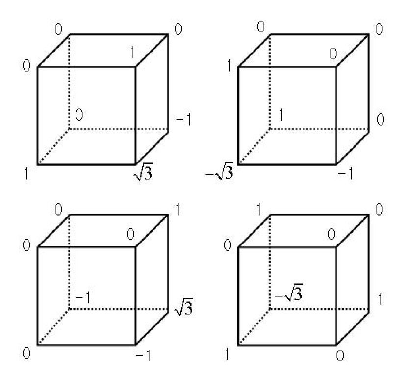
Figure 13: Four degenerate eigenmodes for the $2\times 2\times 2$ unit cell of the ordered state with ${\bf f}=(1/2,1/2,1/2)$, corresponding to the mean-field transition temperature $T_{c}^{\mathrm{MF}}=\sqrt{3}/2\ J/k_{\mathrm{B}}$. The numbers represent the order parameters $\eta_{i}$ of the mode, as indicated in Eq. (39). The phases reside on the nodes of the lattice.

In the mean-field approximation, $T_{c}$ is the highest value of $T$ such that Eq. (39) has a nontrivial solution. With our frustration ${\bf f}=(1/2,1/2,1/2)$, the Hamiltonian is periodic with a unit cell of $2\times 2\times 2$, which implies that Eq. (39) is a set of eight coupled homogeneous linear equations. $T_{c}$ is given by the condition that the determinant of the matrix of coefficients should vanish. This requirement leads to two values of $T^{\prime}=\pm\sqrt{3}/2\sim 0.866$; each is fourfold degenerate. Thus, the transition temperature in the mean-field approximation is $T_{c}^{\mathrm{MF}}=0.866J/k_{\mathrm{B}}$. The four degenerate eigenmodes corresponding to this eigenvalue are $(0,-1,1,\sqrt{3},0,0,0,1)$, $(1,0,-\sqrt{3},-1,0,0,1,0)$, $(-1,\sqrt{3},0,-1,0,1,0,0)$, and $(-\sqrt{3},1,1,0,1,0,0,0)$; these modes are shown in Fig. 13. Of course, any linear combination of these modes would also be an eigenmode. Since the four eigenmodes are degenerate, they must be related by some discrete symmetry operations of the lattice. Thus, we might expect that there are several degenerate ground states. Indeed, our simulations at very low temperatures ($T=0.01J/k_{\mathrm{B}}$) do suggest that the system can readily fluctuate among several different states at such temperatures.

IV Discussion

We have investigated the phase transition in a fully frustrated 3D XY model on a simple cubic lattice, corresponding to an applied magnetic field ${\bf H}=(\Phi_{0}/a^{2})(1/2,1/2,1/2)$. In contrast to the case ${\bf f}=(1/3,1/3,1/3)$ as in Ref. hwang , we see a continuous phase transition. We also extract the critical exponent ratios $\alpha/\nu=0.87\pm 0.01$, $v/\nu=0.82\pm 0.01$, and, with less accuracy, $\nu$ itself, using a variety of numerical techniques. We get $\alpha=0.63\pm 0.07$, $v=0.59\pm 0.07$, and $\nu=0.72\pm 0.07$.

It is of some interest to compare these values with those of other models. In the isotropic (unfrustrated) 3D XY model, $\nu\sim 0.66-0.67$ li1 ; gottlob ; janke ; fernandez ; schultka ; nguyen1 ; ryu ; nho ; krech ; vestergren , $\alpha\approx 0$ gottlob ; janke ; ryu ($\alpha=-0.017$ in Ref. schultka ), and $v\simeq\nu$ li1 ; gottlob ; ryu ; nguyen1 . For the anisotropic but unfrustrated XY model in $d=3$, Ref. nguyen2 reported that $\alpha\sim-0.007$. In the weakly frustrated XY model in $d=3$ (${\bf f}=(0,0,f)$, with $f\leq 1/12$), it has been reported that $\nu\approx 1.5$ nguyen2 . Reference kawamura1 found that $\nu=2.2\pm 0.4$ in a random-coupling 3D XY model with free boundary conditions and ${\bf f}=(0,0,1/2\pi)$, while Ref. kawamura2 found that $\nu=1.1\pm 0.2$ in a random-coupling 3D XY model with periodic boundary conditions and ${\bf f}=(0,0,1/4)$. Our value of $\nu$ satisfies the usual trend that $\nu$ becomes larger than $0.66-0.67$ when the magnetic field is nonzero. However, our results appear not to satisfy the two hyperscaling laws $\alpha=2-d\nu$ and $v=(d-2)\nu$. Possibly the reason is that at this phase transition, two order parameters go to zero: the helicity modulus, and a discrete, Ising-like order parameter related to the amplitude of the structure factor at a characteristic wave vector.

The $T_{c}$ we obtain from the PRG method for $\gamma$ agrees very well with that found from the RGT method, and quite well also with that estimated from $C_{V}(T)$. It is, however, about $20\%$ lower than that obtained by the mean-field approximation. This deviation is not a surprise, because the Monte Carlo $T_{c}$ has been shown to be lower than that found by mean-field theory in other frustrated XY systems shih1 .

In order to avoid the problem of critical slowing down, instead of just increasing the number of Monte Carlo steps, one might attempt to use the cluster flipping algorithm, as first proposed by Swendsen and Wang swendsen , and later by Wolff wolff , and many others edwards ; niedermayer ; kandel ; kawashima ; cataudella2 ; machta . This algorithm is very successful in reducing critical slowing down for unfrustrated models such as the $O(n)$ $\sigma$ model and the Potts model. But when the system is frustrated, especially fully frustrated, a mere extension of the cluster algorithm does not reduce the critical slowing down, and may even increase the correlation time cataudella . The reason is that the cluster percolation temperature $T_{p}$ is much larger than $T_{c}$ in the frustrated system, rendering the cluster flipping trivial at $T_{c}$ because the percolating cluster takes up almost the entire system. Therefore, the cluster should be generated in such a way that $T_{p}$ is closer to $T_{c}$ cataudella ; cataudella2 . Critical slowing down might also be reduced if the standard Metropolis algorithm is combined with the cluster algorithm, resulting in a hybrid algorithm nho ; peczak ; krech .

The renormalization group transformation method is based on certain assumptions which may lead to systematic errors newman5 . Specifically, it assumes that the blocked system has a typical phase configuration of another 3D XY model on a simple cubic lattice with $L^{\prime}=L/b$, i.e., that they appear with the correct Boltzmann probabilities as the original states. This assumption is not exactly correct, and contributes to some systematic error, which cannot be easily estimated. In the present paper, we have tried to estimate these errors using the jackknife method. The renormalization group method is also affected by finite-size effects, because the original system has a different size than does the rescaled system. To optimize the benefits of this method, therefore, we should ideally run simulations on as large a system as possible. We should also do an extra simulation on a system whose size is the same as that of the rescaled system, and compare the two results.

We also comment briefly on the difference between our work and that of Diep et al. diep . These authors did not compute the helicity modulus, nor did they comment on the connection between the model and a superconducting array in a magnetic field. In addition, because of the several techniques described above, we are able to get more accurate values of the ratio $\alpha/\nu$, as well as values for $v/\nu$ and of $\nu$ itself.

Finally, we briefly discuss the possibility that the phase transition at $T_{c}$ might actually be two separate phase transitions. In the 2D fully frustrated XY model, as already mentioned, there are indeed two separate phase transitions: a KT transition at a lower temperature, followed by an Ising-like transition at a slightly higher temperature olsson ; korshunov between a state in which the vortices are ordered in a checkerboard pattern and a disordered vortex state. In the present case, the transition at $T_{c}$ also involves the nearly simultaneous disappearance of 3D XY order (signaled by the vanishing of the helicity modulus) and a discrete order parameter (indicated by the vanishing of the vortex structure factor). Once again, in 3D, the discrete order is characterized by a checkerboard configuration of the vortex state below $T_{c}$ (see Figs. 5–7), although in this case the discrete order parameter is described by four degenerate modes, as determined by the mean-field solution, rather than two as in the 2D fully frustrated XY model choi2 .

Although the discrete and XY order appear to vanish at the same temperature in 3D, and there is no evidence of two separate phase transitions, we believe that our numerical results are not sufficient to conclusively rule out two separate phase transitions. In particular, we have not carried out careful numerical studies of the critical behavior of the discrete order parameter. It would be of interest to carry out further numerical studies, especially of the discrete order parameter, to answer this question definitively.

To summarize, we have studied the phase transition in the fully frustrated XY model, using Monte Carlo simulations in conjunction with two types of real-space renormalization group approaches. We find, in agreement with previous work, that the phase transition is continuous, and we obtain accurate values of the critical exponents $\alpha/\nu$ and $v/\nu$, and a slightly less accurate value for $\nu$ itself. The phase transition could, in principle, be probed experimentally in a suitable three-dimensional lattice of coupled superconducting grains, and possibly also in an assembly of cold atoms in an optical lattice.

$L$	$\tau(t_{\mathrm{MC}})$
4	14
6	29
8	53
10	94
12	148
14	164
16	352

TABLE I: Calculated correlation time $\tau$ for several lattice sizes $L$, evaluated at $T_{c}(L)$. $\tau$ is measured in the units of MC steps per site.

FIGURES

Figure 1: Log-log plot of the data in Table I, corresponding to a fit of $\tau$ to the function $\tau=AL^{z}$. The slope of the fitting line to the data yields the dynamic exponent $z=2.23\pm 0.14$.

Figure 2: Internal energy per site as a function of temperature $T$ for several lattice sizes, as indicated. Note that $T$ decreases with increasing distance along the horizontal axis.

Figure 3: The specific heat per site $C_{V}$ as a function of temperature for several lattice sizes. The lines are cubic spline fits to the data.

Figure 4: The averaged helicity modulus $\gamma=(\gamma_{xx}+\gamma_{yy}+\gamma_{zz})/3$ as a function of temperature for several lattice sizes.

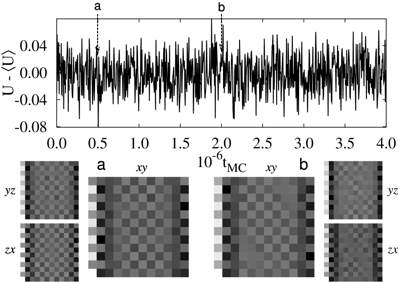
Figure 5: Internal energy per site for a lattice of size $12\times 12\times 12$ as a function of MC time, at the transition temperature $T_{c}=0.681J/k_{\mathrm{B}}$. The intensity plots $a$ and $b$ represent the vortex density-density correlation functions $g_{zz}(x,y,L_{z}/2)$, $g_{xx}(L_{x}/2,y,z)$, and $g_{yy}(x,L_{y}/2,z)$ denoted by $xy$, $yz$, and $zx$, respectively, at the times $a$ and $b$ in the energy evolution curve. A lighter color represents a larger value of the correlation function.

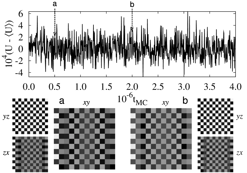
Figure 6: Same as Fig. 5, except that the lattice is at a very low temperature $T=0.01J/k_{\mathrm{B}}$.

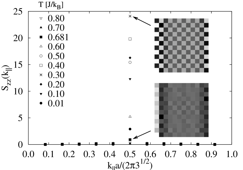
Figure 7: Vortex structure factor $S_{zz}(k_{\parallel})$ parallel to the applied magnetic field at several temperatures for a lattice of size $12\times 12\times 12$ and periodic boundary conditions. The insets are the vortex density-density correlation functions $g_{zz}(x,y,L_{z}/2)$ at two different temperatures $T=0.30J/k_{\mathrm{B}}$ (top) and $T=0.681J/k_{\mathrm{B}}$. A lighter color represents a larger value of the correlation function.

Figure 8: MC probability distribution $P(U)$ for the internal energy per site $U$ at the transition temperature $T_{c}=0.681J/k_{\mathrm{B}}$ for several lattice sizes.

Figure 9: Log-log plot of the maximum height $C_{V}$ of the specific heat per site versus linear size $L$ of the lattice. The points are MC data; the full curve is the best-fit line. The slope of the fit line gives $\alpha/\nu=0.87\pm 0.01$.

Figure 10: Log-log plot of the helicity modulus $\gamma$ versus linear size $L$ of the lattice. The points are MC data at two different temperatures $T=0.681J/k_{\mathrm{B}}$ and $T=0.682J/k_{\mathrm{B}}$; the full curves are the best-fit lines. The slopes of the fit lines give $v/\nu=0.79\pm 0.02$ at $T=0.681J/k_{\mathrm{B}}$ and $v/\nu=0.83\pm 0.02$ at $T=0.682J/k_{\mathrm{B}}$. The error bars from the jackknife method are smaller than the symbol sizes.

Figure 11: PRG method to extract the transition temperature $T_{c}$ and the critical exponent $v/\nu$ of the helicity modulus $\gamma$. All three curves show $\gamma(L,t)/\gamma(L^{\prime},t)$ for the same ratio of $L/L^{\prime}=2$. The $x$ and $y$ coordinates of the intersection of the three curves yield the values of $T_{c}$ and $(L/L^{\prime})^{-v/\nu}$.

Figure 12: RGT method to extract the transition temperature $T_{c}$ and the critical exponent $\nu$ of the correlation length. The ratio of the slopes of the two fitting lines at $T_{c}$ gives the value of $\nu$, according to Eq. (37).