Internal Energy of the Potts model on the Triangular Lattice with Two- and Three-body Interactions

Abstract

We calculate the internal energy of the Potts model on the triangular lattice with two- and three-body interactions at the transition point satisfying certain conditions for coupling constants. The method is a duality transformation. Therefore we have to make assumptions on uniqueness of the transition point and that the transition is of second order. These assumptions have been verified to hold by numerical simulations for $q=2$, $3$ and $4$, and our results for the internal energy are expected to be exact in these cases.

1 Introduction

Exact solutions have exerted strong influences on the development of statistical physics of equilibrium systems, the spin models in particular. Among useful techniques for this purpose, one is the duality transformation, which applies mainly to two-dimensional cases. Ever since the first formulation of duality by Kramers and Wannier[1], the method has been used to predict the transition points of the Ising model on the square lattice[1], the Potts model on the square, [2, 3] triangular, and hexagonal lattices[4]. The duality transformation makes it possible to obtain the location of the transition point if it is unique. We can also calculate the internal energy at the transition point for a self-dual model from the derivative of the duality relation[3, 5].

In the presented paper, we apply the duality transformation to the Potts model with two- and three-body interactions on the triangular lattice and calculate the internal energy at the transition point. The Potts model with two- and three-body interactions on the triangular lattice was first introduced by Kim and Joseph[4]. They obtained this model as a result of an application of the duality and star-triangle transformations to the Potts model only with two-body interactions on the triangular lattice. Later, Baxter, Temperly and Ashley showed algebraically that the Potts model with two- and three-body interactions is self-dual[6], and so also did Wu and Lin graphically[7]. It was also shown that the Potts model with only three-body interactions on the triangular lattice is self-dual[6], though the Potts model with only two-body interactions is not.

Baxter, Temperley and Ashley obtained the exact solution for the free energy and the internal energy of the Potts model at the transition point with two-body interactions on the triangular lattice[6]. They used the relationship between this Potts model and the soluble Kelland model. However, it was difficult to analyze the Potts model with both two- and three-body interactions whereas the model is amenable to exact analysis by duality if it has only three-body interactions[6]. The Potts model with two- and three-body interactions has not been treated by such considerations, because of the complexity of the relationship between the original model and its dual although the duality for this model has been well known.

Our goal is to derive the exact solution of the internal energy at the transition point for the Potts model with two- and three-body interactions using the duality transformation. We find that the duality transformation gives us the value of the internal energy only on some special points, which lie on the line of transition points. We also discuss the mechanism that we can calculate the internal energy by the duality transformation.

The outline of the presented paper is as follows. Section $2$ gives a brief introduction to the Potts model with two- and three-body interactions on the triangular lattice and its duality transformation. Here we will find the condition that we can calculate the internal energy by use of the duality transformation. In §$3$, we numerically verify the results obtained in §$2$. The last section is devoted to discussions.

2 Energy of the Potts model with two- and three-body interactions

We introduce the $q$-state Potts model with two- and three-body interactions on the triangular lattice and write its duality relations, following Ref. Wu2). The Hamiltonian is

$$H(J_{2},J_{3})\equiv\sum_{\bigtriangleup}H_{\bigtriangleup}(J_{2},J_{3})=-J_{2}\sum_{\bigtriangleup}\sum_{i\neq j}\delta\left(\phi_{i},\phi_{j}\right)-J_{3}\sum_{\bigtriangleup}\delta\left(\phi_{1},\phi_{2},\phi_{3}\right),$$ (1)

where {$\phi_{i}$} denotes the spin variables ($\phi_{i}=0,1,\cdots,q-1$). The summation in the second expression is over all up-pointing triangles as shown in Fig. 1. Three-body interactions exist only on the up-pointing triangles. Therefore our model is slightly different from the model of Schick and Griffiths[9], which has three-body interactions on all up-pointing and down-pointing triangles. The summation in the third expression with subscript $i\neq j$ is over bonds $(1,2)$, $(2,3)$ and $(3,1)$ around each up-pointing triangle as shown in Fig. 1. The strengths of the two- and three-body interactions are denoted as $J_{2}$ and $J_{3}$, and $\delta$ is the Kronecker’s symbol.

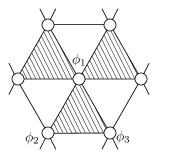
Figure 1: The Potts model with two- and three-body interactions on the triangular lattice. Each of the spin variables interacts with nearest-neighboring sites (two-body interactions). We also consider three-body interactions among spins on all up-pointing triangles as shown shaded.

The partition function is written as

$$Z(K_{2},K_{3})=\sum_{\{\phi_{i}\}}\exp\left\{-\beta H(J_{2},J_{3})\right\}=\sum_{\{\phi_{i}\}}\prod_{\bigtriangleup}\exp\left\{K_{2}\sum_{i\neq j}\delta\left(\phi_{i},\phi_{j}\right)+K_{3}\delta\left(\phi_{1},\phi_{2},\phi_{3}\right)\right\},$$ (2)

where $K_{2}=\beta J_{2}$ and $K_{3}=\beta J_{3}$. This model is self-dual and the duality relation is known to be [6, 7, 8]

$$Z(K_{2},K_{3})=\left(\frac{y}{q}\right)^{N}Z(K^{*}_{2},K^{*}_{3}),$$ (3)

where $K^{*}_{2}$ and $K^{*}_{3}$ are the dual coupling constants and $N$ is the number of sites, which is the same as the number of up-pointing triangles. The relations between the coupling constants $(K_{2},K_{3})$ and $(K^{*}_{2},K^{*}_{3})$ are

$$v^{*}=\frac{qv}{y},\quad y^{*}=\frac{q^{2}}{y},$$ (4)

where $v\equiv e^{K_{2}}-1$ and $y\equiv e^{K_{3}+3K_{2}}-3e^{K_{2}}+2$ and similarly for $v^{*}$ and $y^{*}$ using $K^{*}_{2}$ and $K^{*}_{3}$. The fixed-point condition, $K_{2}=K^{*}_{2}$ and $K_{3}=K^{*}_{3}$, is equivalent to $y=q$, which describes a line in the $(K_{2},K_{3})$ plane. It is expected that the system undergoes a phase transition across the line $y=q$. Indeed Wu and Zia argued that the line $y=q$ represents the critical surface if $J_{3}+3J_{2}>0$ and $J_{3}+2J_{2}>0$ [10].

Next let us calculate the internal energy on the line $y=q$, using the duality relation of the partition function (3). In the case of a simple single-variable duality $Z(K)=c(K)^{N}Z(K^{*})$, the logarithmic derivative of both sides readily leads to the energy at the fixed-point,

$$e(K_{c})=-\frac{1}{c\left(1-\displaystyle\frac{dK^{*}}{dK}\right)}\left.\frac{dc}{dK}\right\rvert_{K=K_{c}},$$ (5)

where $e(K)$ is the energy per site, under the assumption of continuity $e(K_{c}+0)=e(K_{c}-0)$. We therefore try to apply the same procedure to the present duality relation (3) with two variables.

The logarithmic derivative of the partition function with respect to $\beta$ gives the internal energy per site as follows;

$$-\frac{1}{N}\frac{\partial}{\partial\beta}\ln Z(K_{2},K_{3}) = -\frac{J_{2}}{N}\left\langle\sum_{\bigtriangleup}\sum_{i\neq j}\delta\left(\phi_{i},\phi_{j}\right)\right\rangle_{K_{2},K_{3}}-\frac{J_{3}}{N}\left\langle\sum_{\bigtriangleup}\delta\left(\phi_{1},\phi_{2},\phi_{3}\right)\right\rangle_{K_{2},K_{3}}$$ (6)

$$\equiv J_{2}U_{2}(K_{2},K_{3})+J_{3}U_{3}(K_{2},K_{3}),$$

where the brackets $\langle\cdots\rangle_{K_{2},K_{3}}$ denote the thermal average. The values of $U_{2}(K_{2},K_{3})$ and $U_{3}(K_{2},K_{3})$ on the line $y=q$ satisfy the following equations, which are obtained by taking logarithmic derivatives of eq. (3) by $K_{2}$ and $K_{3}$ and assuming continuity (i. e. second-order transition) of these derivatives across the line $y=q$,

$$\left\{1-\left.\left(\frac{\partial K_{2}^{*}}{\partial K_{2}}\right)\right\rvert_{y=q}\right\}U_{2}-\left.\left(\frac{\partial K_{3}^{*}}{\partial K_{2}}\right)\right\rvert_{y=q}U_{3} = \frac{1}{q}\left.\left(\frac{\partial y}{\partial K_{2}}\right)\right\rvert_{y=q}$$ (7)

$$-\left.\left(\frac{\partial K_{2}^{*}}{\partial K_{3}}\right)\right\rvert_{y=q}U_{2}+\left\{1-\left.\left(\frac{\partial K_{3}^{*}}{\partial K_{3}}\right)\right\rvert_{y=q}\right\}U_{3} = \frac{1}{q}\left.\left(\frac{\partial y}{\partial K_{3}}\right)\right\rvert_{y=q}.$$ (8)

It turns out that these two equations are not independent of each other as proved in AppendixA. Because of this property, we cannot calculate both $U_{2}$ and $U_{3}$ from eqs. (7) and (8), which makes it difficult in general to evaluate eq. (6). Nevertheless, if the left-hand side of eq. (7) is proportional to the final expression of eq. (6), eq. (7) gives the internal energy apart from the proportionality constant (which can be calculated from the values of coefficients $U_{2}$ and $U_{3}$ in eq. (7)). We therefore require that the ratio of coefficients of $U_{2}$ and $U_{3}$ in eq. (7), $\{1-(\partial K_{2}^{*}/\partial K_{2})\rvert_{y=q}\}/\{-(\partial K_{3}^{*}/\partial K_{2})\rvert_{y=q}\},$ equal to $J_{2}/J_{3}$:

$$J_{3}\left\{1-\left.\left(\frac{\partial K_{2}^{*}}{\partial K_{2}}\right)\right\rvert_{y=q}\right\}=-J_{2}\left.\left(\frac{\partial K_{3}^{*}}{\partial K_{2}}\right)\right\rvert_{y=q}.$$ (9)

We can write this condition explicitly in terms of $K_{2}$ and $K_{3}$, using the explicit forms of the derivatives in eqs. (15) and (17) in AppendixA, as follows,

$$(J_{3}+3J_{2})\frac{v_{c}(6v_{c}+3q)}{q(1+v_{c})}=J_{2}\left[3-\frac{1}{3v_{c}+q+1}\left\{3(1+v_{c})-(3v_{c}+q)\frac{6v_{c}+3q}{q}\right\}\right],$$ (10)

where $v_{c}=e^{K_{2}}-1$ with $K_{2}$ being the value on the line $y=q$. This equation is reduced to

$$(K_{3}+3K_{2})(3e^{K_{2}}+q-2)(e^{K_{2}}-1)=K_{2}(3e^{K_{2}}+2q-3)e^{K_{2}}.$$ (11)

where $K_{3}$ is the value on the line $y=q$. We can calculate the internal energy at the limited points on the line $y=q$ determined by eq. (11).

Let us emphasize once again that the condition (11) for the internal energy to be calculable has been obtained under the assumption of uniqueness and continuity of the transition. The former uniqueness assumption was used in the identification of the fixed point $y=q$ with the transition point as discussed in Ref. Wu3), and the latter continuity was necessary in deriving eqs. (7) and (8).

3 Results and numerical verification

Equation (11) with $y=q$ has solutions for $q=2,3$ and $4$ as well as for $q\geq 69$. The results for the former case are listed in Table 1.

$q$	$K_{2}$	$K_{3}$	$\tau$	energy
$2$	$0.375530$	$0.347552$	$0.925497$	$-3.19412$
$3$	$0.291622$	$0.737724$	$2.52973$	$-3.95336$
$4$	$-0.062177$	$1.75913$	$-28.2924$	$-15.5884$
$4$	$-1.09861$	$4.39445$	$-4$	$-0.5$

Table 1: Solutions of eq. (11) and $y=q$. Here $\tau\equiv K_{3}/K_{2}$.

The values of coupling constants in Table 1 satisfy the Wu-Zia criteria $J_{3}+3J_{2}>0$, and $J_{3}+2J_{2}>0$, which means that the existence of a transition in each case is very plausible. We have checked the assumption of uniqueness and continuity of the transition by numerical simulations for $q=2$, $3$ and $4$. Systems with larger $q$ are expected to have first-order transitions since the Potts model with two-body interactions on the square lattice has first order transition for $q\geq 5$[8]. We thus have not carried out numerical simulations for the case of larger $q$.

Most simulations have been performed for linear system size $100$ and $10500$ MCS per spin. The data have been averaged over $100$ independent runs. The exception is the case with $q=4$ and $\tau=K_{3}/K_{2}=-4$, in which we took $250$ independent runs of $4500$ MCS.

The results are shown in Fig. 2 for $q=2$, $3$ and $4$ (with $\tau=-28.2924$) and Fig. 3 for $q=4$ with $\tau=-4$. In Fig. 2 we observe that the internal energy shows no hysteresis, which suggests that the assumption of continuity of transition is valid. It is also seen that the duality predictions for the energy agree well with numerical data. In contrast, the case with $q=4$ and $\tau=-4$ seems to undergo a first-order transition as is seen in Fig. 3. Thus the solution given in Table 1 for $q=4$ and $\tau=-4$ would correspond to the average of $e(K_{c}+0)$ and $e(K_{c}-0)$, which is compatible with data in Fig. 3: In the case of a simple self duality $Z(K)=c(K)^{N}Z(K^{*})$, taking the limit $K\to K_{c}+0$ after the logarithmic derivative leads to the average of $e(K_{c}+0)$ and $e(K_{c}-0)$ on the left-hand side of eq. (5). The same situation is expected for $q=4$ and $\tau=-4$.

Figure 2: The internal energy at the fixed points of duality as in Table. 1 except for $q=4$, $\tau=-4$. The symbol ‘inc’ denotes the internal energy measured by increasing the temperature, ‘dec’ stands for the results by decreasing temperature, and ‘dual’ is for our duality results.

Figure 3: The internal energy of the four-state Potts model with $\tau=-4$. The same symbols are used as in Fig. 2.

4 Discussions

We have calculated the internal energy of the Potts model on the triangular lattice with two- and three-body interactions satisfying certain conditions for coupling constants. These results have been obtained from duality under the assumptions on uniqueness of the transition point and that the transition is of second order. We checked these assumptions by Monte Carlo simulations. It has been shown that the assumptions are valid for $q=2$, $3$ and $4$ ($\tau=-28.2924$) but not for $q=4$ ($\tau=-4$). In the former case it is expected that the duality predictions are exact. In the latter case our result gives the average energy above and below the transition point.

It is possible to understand the condition (11) for the internal energy to be calculable from a little different point of view. In Fig. 4, $\tau=K_{3}/K_{2}$ and the dual $\tau^{*}=K^{*}_{3}/K^{*}_{2}$ are plotted as functions of $K_{2}$.

Figure 4: The behaviors around the solutions of eq. (11). The horizontal solid line is the original model and the dashed line is for $K_{3}^{*}/K_{2}^{*}$. These two lines intersect at the fixed point ($y=q$) shown in black dot.

As seen there, the two lines have the same slope (i.e. both are flat) at the fixed point. This feature $dK^{*}_{3}/dK^{*}_{2}=dK_{3}/dK_{2}$ can be verified by direct manipulations of the conditions (7)-(11). In this sense the solvability condition may be regarded as a condition for the dual model to be the same model as the original one, i.e., the same ratio of coupling constants between two- and three-body interactions. In other words the model is self-dual in a very strict sense only at the transition point for $q=2$, $3$ and $4$ ($\tau=-28.2924$).

It is interesting to see the case of $q=4$, $\tau=-4$ in Fig. 4: the model is self-dual even away from the transition point. This is a very interesting special feature of this case.

5 Acknowledgement

This work was partially supported by a 21st Century COE Program at Tokyo Institute of Technology ‘Nanometer-Scale Quantum Physics’ by the Ministry of Education, Culture, Sports, Science and Technology and by CREST, JST.

Appendix A Evaluation of the determinant

In this Appendix we show that eqs. (7) and (8) are not independent. The dual coupling constants $K^{*}_{2}$ and $K^{*}_{3}$ are expressed by $y$ and $v$ as follows

$$K^{*}_{2} = \log\left(1+\frac{qv}{y}\right)$$ (12)

$$K^{*}_{3} = -3K_{2}^{*}+\log\left(1+\frac{3qv+q^{2}}{y}\right),$$ (13)

where $y=e^{K_{3}+3K_{2}}-3e^{K_{2}}+2$ and $v=e^{K_{2}}-1$. On the line $y=q$ , the derivatives of $y$ and $v$ are seen to satisfy

$$\frac{\partial y}{\partial K_{2}}=6v_{c}+3q,\quad\frac{\partial y}{\partial K_{3}}=3v_{c}+1+q,\quad\frac{\partial v}{\partial K_{2}}=1+v_{c},\quad\frac{\partial v}{\partial K_{3}}=0,$$ (14)

where $v_{c}\equiv e^{K_{2c}}-1$. From these relations, we can obtain the derivatives of $K^{*}_{2}$ and $K^{*}_{3}$ with respect to $K_{2}$ and $K_{3}$ on the $y=q$ line as follows

$$\left.\frac{\partial K_{2}^{*}}{\partial K_{2}}\right\rvert_{y=q} = 1-\frac{v_{c}(6v_{c}+3q)}{q(1+v_{c})}$$ (15)

$$\left.\frac{\partial K_{2}^{*}}{\partial K_{3}}\right\rvert_{y=q} = \frac{-v_{c}(3v_{c}+1+q)}{q(1+v_{c})}$$ (16)

$$\left.\frac{\partial K_{3}^{*}}{\partial K_{2}}\right\rvert_{y=q} = -3\left.\frac{\partial K_{2}^{*}}{\partial K_{2}}\right\rvert_{y=q}+\frac{1}{3v_{c}+q+1}\left\{3(1+v_{c})-(3v_{c}+q)\frac{6v_{c}+3q}{q}\right\}$$ (17)

$$\left.\frac{\partial K_{3}^{*}}{\partial K_{3}}\right\rvert_{y=q} = -3\left.\frac{\partial K_{2}^{*}}{\partial K_{3}}\right\rvert_{y=q}-\frac{(3v_{c}+q)}{q}.$$ (18)

Using these derivatives, the determinant of eqs. (7) and (8) is evaluated as

$$\left(1-\left.\frac{\partial K_{2}^{*}}{\partial K_{2}}\right\rvert_{y=q}\right)\left(1-\left.\frac{\partial K_{3}^{*}}{\partial K_{3}}\right\rvert_{y=q}\right)-\left.\frac{\partial K_{3}^{*}}{\partial K_{2}}\right\rvert_{y=q}\left.\frac{\partial K_{2}^{*}}{\partial K_{3}}\right\rvert_{y=q}$$

$$=\frac{v_{c}(6v_{c}+3q)}{q(1+v_{c})}\left\{1+3\frac{-v_{c}(3v_{c}+1+q)}{q(1+v_{c})}-\frac{(3v_{c}+q)}{q}\right\}$$

$$\quad-\frac{-v_{c}(3v_{c}+1+q)}{q(1+v_{c})}\left[-3\left\{1-\frac{v_{c}(6v_{c}+3q)}{q(1+v_{c})}\right\}+\frac{1}{3v_{c}+q+1}\left\{3(1+v_{c})-(3v_{c}+q)\frac{6v_{c}+3q}{q}\right\}\right]$$

$$=0.$$

Thus eqs. (7) and (8) are not independent.

References

- [1] H. A. Kramers and G. H. Wannier: Phys. Rev. 60 (1941) 252.
- [2] R. B. Potts: Proc. Camb. Phil. Soc. 48 (1952) 106.
- [3] T. Kihara, Y. Midzuno, and T. Shizume: J. Phys. Soc. Jpn. 9 (1954) 681.
- [4] D. Kim and R. I. Joseph: J. Phys. C: Solid State Phys. 7 (1974) L167.
- [5] I. Syozi: in Phase transition and Critical Phenomena, Vol. 1, Eds. C. Domb and M. S. Green (Academic Press, 1972).
- [6] R. J. Baxter, H. N. V. Temperly and S. E. Ashley: Proc. R. Soc. A358 (1978) 535.
- [7] F. Y. Wu and K. Y. Lin: J. Phys. A: Math. Gen. 13 (1980) 629.
- [8] F. Y. Wu: Rev. Mod. Phys. 54 (1982) 235.
- [9] M. Schick and R. B. Griffiths: J. Phys. A: Math. Gen. 10 (1977) 2123.
- [10] F. Y. Wu and R. K. P. Zia: J. Phys. A: Math. Gen. 14 (1981) 721.