Magnetic disorder and dynamical properties of a Bose-Einstein condensate in atomic waveguides

Abstract

We systematically investigate the properties of the quenched disorder potential in an atomic waveguide, and study its effects to the dynamics of condensate in the strong disorder region. We show that even very small wire shape fluctuations can cause strong disorder potential along the wire direction, leading to the fragmentation phenomena as the condensate is close to the wire surface. The generic disorder potential is Gaussian correlated random potential with vanishing correlations in both short and long wavelength limits and with a strong correlation weight at a finite length scale, set by the atom-wire distance. When the condensate is fragmentized, we investigate the coherent and incoherent dynamics of the condensate, and demonstrate that it can undergo a crossover from a coherent condensate to an insulating Bose-glass phase in strong disorder (or low density) regime. Our numerical results obtained within the meanfield approximation are semi-quantitatively consistent with the experimental results.

I Introduction

Low dimensional physics has long been an important and extensively studied subjects in condensed matter physics since the early theoretical interest in 60th. In addition to the ordinary solid state system, e.g. semi-conductor quantum wells, quantum wires, carbon nanotubes, and organic conductors etc., systems of ultracold atoms in highly anisotropic magneto-optical traps have been also a promising new system for the low dimensional physics of both fermion and boson particles ketterle ; petrov ; stoof . Among varies proposals of the anisotropic magneto-optical traps, microfabricated magnetic trap, also called atomic waveguide or microtrap microchip_general , has an additional important advantage for the coherent transport of atoms along the quasi-one-dimensional (Q1D) waveguide potential (for a typical system setup, see Fig. 1(a) and the description in the next section). Such combination of ultracold atoms in quantum mechanical limit with the great versatility of the fabrication technique has opened a new direction to study many Q1D quantum physics, like coherent transport aaron1 , beam splitter beamsplitter , interference of matter wave interference , and Tonks gas limit tonks . Many theoretical works have been proposed in the literature to study these aspects in very recent years.

From experimental point of view, however, in order to successfully trap ultracold atoms in the atomic waveguide, one has to apply very strong confinement potential in the transverse dimension, which is usually achieved by moving atoms very close to the conducting wire on the substrate. (Electric current in the wire cannot be too large in order to avoid heating private .) When the atom-wire distance is smaller than some critical values, which is usually about $100-200$ $\mu$m, however, nontrivial atom density modulation (fragmentation) of the condensate occurs, as have been observed by different groups aaron1 ; aaron2 ; zimmermann1 ; kraft02 ; hinds . It is also found that atom could cannot be transported without excitations to higher energy band when such fragmentation occurs inside the cloud aaron1 ; transport . For a static fragmentized atom cloud, it shows a rather generic (but not universal) length scale, $\lambda$, in $z$ direction, which becomes smaller when $d$ is reduced. Kraft et. al. kraft02 further observe that the positions of atom density maximum/minimum can be exchanged if the direction of the offset magnetic field is reversed, showing a nontrivial quenched disorder effects in the microtrap system. Such interesting disorder effects can be very crucial when considering the coherent transport in the magnetic waveguide, and was first investigated theoretically by us recently early_work . We note that such quenched disorder induced fragmentation phenomena is different from the thermal fluctuation studied in Ref. henkel . The thermal fluctuation effects can be neglected in our present scope of interest, because it becomes prominent only when the atoms are even closer to the wire surface (say $d<20$ $\mu$m), while the fragmentation phenomena occur at well-larger distance (say $d<200$ $\mu$m).

The disorder effects in an interacting bosonic system have been an interesting subject in the context of liquid helium system for decades. In weak disorder limit, it is believed that the disorder effects is irrelevant to the ground state properties due to the strong repulsive interaction between bosons in two and three dimensional systems huang ; stringari_disorder ; nelson97 ; lopatin02 . Similar conclusion also applies to one-dimensional (1D) bosonic system giamarchi . However, when the disorder strength increases, it is argued by Fisher et al. that the system can undergo a quantum phase transition to a ”Bose-glass” phase fisher , which breaks the usual $U(1)$ symmetry of bosons to have a condensate but is insulating due to disorders. However, the existence of the ”Bose-glass” phase in the liquid helium system is still unclear in the present experimental data reppy .

However, the invention of optical lattice for trapping ultracold atoms provides another route to study the disorder effects to the bosonic systems. Experimentalists uses laser of different frequency to produce an artificial random potential (speckle pattern) and study the ground state or transport properties of cold atoms zoller ; optical_lattice . Recently, the onset of Bose glass regime is observed near the Mott-insulator regime bose_glass .

In this paper, we extend our earlier work early_work and provide a more detailed study on the origin, properties, and effects of disorder potential in atomic waveguide system. We show a first principle and quantitative theory to describe the disorder potential in the atomic waveguide, and demonstrate that even a very small wire shape fluctuation can cause a strong disorder field, which has a correlation function that vanishes at small and infinite wavevectors and is peaked at a wavevector, $k_{c}$ with a length scale determined by the atom-wire distance ($d$). We note that similar analytical works and numerical comparison with experimental data have been also studied recently aspect1 ; aspect2 after our work. In strong disorder regime, the condensate becomes fragmentized as observed in the experiment aaron1 ; aaron2 ; zimmermann1 ; kraft02 ; hinds . We then concentrate on the dynamical response of the condensate in the shaking experiment and propose that a quantum phase transition from a superfluid state to an insulating Bose glass state may be observed in the parameter regime of current experiments. Our results provide a good starting point of the disorder effects to the coherent transport and to the low dimensional Bose systems in the future development.

This paper is organised as follows: In Section II we present the theory of the magnetic disorder potential generated from the wire shape distortion in the microchip system. In Section III, we study the condensate fragmentation in strong disorder region. Then we discuss the finite temperature effects and other details in Sec. IV and summarize our results in Section V.

II Disordered magnetic field

In Fig. 1(a) we show a typical experimental setup of an atomic waveguide: ultra-cold atoms are loaded into the microtrap, which is composed by a radiant magnetic field gradient (generated by the electric current in a one-dimensional microfabricated copper wire) and a uniform bias field, $B_{\perp}$, in the transverse direction ($y$). Atoms are confined at the potential minimum with a distance $d=\frac{2I_{0}}{cB_{\perp}}$ to the wire center (in c.g.s. unit), where $B_{\perp}$ exactly cancels the field of the wire current. A uniform offset field, $B_{\|}$, is applied parallel in the wire direction ($z$) to reduce the trap loss by polarizing the atom spins. Additional magnetic field gradients can be also applied in $z$ direction to confine the atoms in the longitudinal direction. The elongated confinement potential can be approximated by a harmonic potential, with confinement frequencies, $\omega_{\perp}$ and $\omega_{\|}$ in $x-y$ and $z$ directions respectively.

II.1 General properties of disordered magnetic field

Before studying the disorder magnetic field generated by the wire shape fluctuations, we think it is helpful to study some more general properties of the disorder magnetic field. Using the fact that the typical Zeeman energy of atoms is very large ($\sim$ MHz), we can safely assume that all atoms are condensed in the lowest spin state (i.e. fully polarized in the direction of the total magnetic field) so that the confinement potential, $U({\bf r})$, is proportional to the total magnetic field:

$$U({\bf r})=\mu_{a}|{\bf B}_{\rm tot}({\bf r})|,$$ (1)

where $\mu_{a}$ is the magnetic dipole moment of atoms and ${\bf B}_{\rm tot}({\bf r})=B_{\|}\hat{z}+B_{\perp}\hat{y}+{\bf B}_{0}({\bf r})+\delta{\bf B}({\bf r})$; $\delta{\bf B}({\bf r})$ is the disorder magnetic field, which will be calculated in details later. Since the condensate in the microchip system is highly elongated in $z$ direction with a very small transverse radius, $R_{TF}\sim 1-5$ $\mu$m, we can neglect the finite size effects for simplicity and just consider the disorder potential at the confinement center $(x,y,z)=(d,0,z)$, where ${\bf B}_{\perp}=B_{\perp}\hat{y}$ cancels the unperturbed azimuthal field, ${\bf B}_{0}$. In the limit of small disorder magnetic field, one can make an expansion of Eq. (1) and obtain:

$$\delta U(z) \sim s_{\|}\mu_{a}\delta B_{z}(z)+\frac{\mu_{a}\left[|\delta{\bf B}(z)|^{2}-2\delta B_{z}(z)^{2}\right]}{2|B_{\|}|},$$ (2)

where $s_{\|}\pm 1$ is the sign of the offset field, $B_{\|}$, in $z$ direction. Note that in Eq. (2) the first (dominant) term is linearly proportional to $\delta B_{z}$, so that $\delta U(z)$ changes sign if the direction of either the electric current or the offset magnetic field is changed. This simple observation explains the experimental results observed in Ref. [kraft02, ], where Kraft et al. find that the positions of local potential maximum/minimum can be exchanged by changing the direction of $B_{\|}$ or the current. The second term of Eq. (2), however, does not change sign for different $B_{\|}$ or current direction, and therefore explain why the density profile of the condensates obtained by opposite directions of current (or opposite $B_{\|}$) are not symmetric. However, since $|B_{\|}|$ is in general much larger than the disorder field ($|\delta{\bf B}/B_{\|}|\ll 0.1\%$ in general), we will simply neglect the second term of Eq. (2) and consider $\delta B_{z}$ only when applying to the realistic disorder field calculation, although we will still derive the disorder magnetic field in all the components of $\delta{\bf B}$ later, which may be useful in considering the finite size effects of BEC in the future study.

In this paper, we consider a microchip system where the magnetic field is generated from a rectangular cooper wire with width $W_{0}$ (in the substrate plane) and hight $H_{0}$ (vertical to the substrate plane, see Fig. 1(a)). The typical scale for the semiconductor wire is $H_{0}\sim 1-5$ $\mu$m, and $W_{0}\sim 3-50$ $\mu$m aaron1 ; zimmermann1 . In general, the wire shape fluctuation can occur in both of these two directions due to the fluctuations during the crystal growth. However, in this paper we assume the width fluctuation or center changes only in the horizontal direction ($y$), but not in the vertical direction ($x$) for simplicity (see Fig. 1). This is a good approximation because the current density in $x$ direction should generate much smaller magnetic field at the position right above the wire according to the Biot-Savart law in classical electrodynamics. Such approximation is also confirmed by the numerical work in Ref. [aspect2, ] after our first analytical study early_work . Therefore we can define the wire shape function, $y=-W_{0}/2+f_{L}(z)$ for the left boundary and $y=W_{0}/2+f_{R}(z)$ for the right boundary of the wire in the substrate ($y-z$) plane, and the current fluctuation becomes in $y-z$ directions only, i. e.

$$\delta{\bf J}(y,z) \sim \delta J_{y}(y,z)\hat{y}+\delta J_{z}(y,z)\hat{z},$$ (3)

which are closely related to the shape of the wire and will be studied in details below.

 

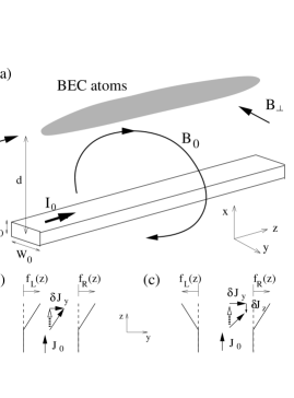
Figure 1: (a) Schematic figure of a BEC loaded in a microtrap. ${\bf B}_{0}({\bf r})$, $B_{\|}\hat{z}$, and $B_{\perp}\hat{y}$ are the azimuthal magnetic field generated by a steady current, the offset field, and the bias field respectively. (b) and (c) present the $C-$ and $W-$ types of wire shape fluctuations respectively.

When studying the current fluctuation in the wire, it is in general tentative to approximate the disorder nature of current fluctuation by the following expectation values henkel

$$\langle\delta{\bf J}({\bf r})\rangle_{\rm dis} = 0$$ (4)

$$\langle\delta J_{\alpha}({\bf r})\delta J_{\beta}({\bf r}^{\prime})\rangle_{\rm dis} = \delta_{\alpha\beta}D({\bf r}-{\bf r}^{\prime}),$$ (5)

where $\alpha,\beta=x,y,z$, $\langle\cdots\rangle_{\rm dis}$ is disorder ensemble average, and $D({\bf r}-{\bf r}^{\prime})$ is the correlation function of the fluctuating current. However, we point out that Eq. (5) is not correct for a normal conduction wire, because it assumes no correlation between different components of the fluctuating current. For any static current distribution, as we will see below, the microscopic continuity equation still applies to the disorder current so that any current fluctuation in one direction should somehow affects the current in other directions. Besides, the total current following in any single wire (i.e. for any specific system as done in the realistic experiment) must be a constant too, not only the ensemble-averaged value is unchanged as implied by Eq. (4). Therefore the realistic current fluctuation should obey some more strict conditions than those shown in Eqs. (4) and (5). This fact will change the disorder nature of the magnetic field significantly as we will show in the rest of this section.

II.2 Current conservation and the boundary conditions

The first step is to introduce the current conservation and the electro-dynamical equations in a self-consistent method. We start from the static version of continuity equation, $\nabla\cdot\delta{\bf J}({\bf r})=0$, which gives

$$\frac{\partial\delta J_{y}(y,z)}{\partial y}+\frac{\partial\delta J_{z}(y,z)}{\partial z}=0.$$ (6)

Another equation can be derived from the Maxwell equation, $\nabla\times{\bf E}=-\partial{\bf B}/\partial t$, with $\partial{\bf B}/{\partial t}=0$ for static current and assuming a constant conductivity, $\sigma$, inside the wire (and zero outside the wire) (i.e. ${\bf J}=\sigma{\bf E}$), so that $\nabla\times{\bf J}=0$ or equivalently:

$$\frac{\partial\delta J_{z}(y,z)}{\partial y}-\frac{\partial\delta J_{y}(y,z)}{\partial z}=0.$$ (7)

Eqs. (6) and (7) are the two equations we have to solve by incorporating the proper boundary conditions.

The first boundary condition is from the total current conservation in $z$ direction, which gives (See Fig. 1(c))

$$I_{0} = \int_{H_{0}/2}^{H_{0}/2}dx^{\prime}\int_{-W_{0}/2+f_{L}(z)}^{-W_{0}/2+f_{R}(z)}dy^{\prime}{\bf J}(y^{\prime},z)\cdot\hat{z}$$ (8)

$$= H_{0}\int_{-W_{0}/2+f_{L}(z)}^{-W_{0}/2+f_{R}(z)}dy^{\prime}\left(J_{0}+\delta J_{z}(y^{\prime},z)\right)$$

$$\sim I_{0}+H_{0}J_{0}\left(f_{R}(z)-f_{L}(z)\right)$$

$$+H_{0}\int_{-W_{0}/2}^{-W_{0}/2}dy^{\prime}\delta J_{z}(y^{\prime},z),$$

where $J_{0}\hat{z}$ is the unperturbed (or average) current density in the wire, $I_{0}=J_{0}W_{0}H_{0}$ is the total current, and in the last equation we have expand the right hand side by assuming small wire shape fluctuation, i.e.

$$|f_{L/R}(z)|\ll W_{0}$$ (9)

In other words, we have

$$J_{0}\left(f_{R}(z)-f_{L}(z)\right) = -\int_{-W_{0}/2}^{-W_{0}/2}dy^{\prime}\delta J_{z}(y^{\prime},z).$$ (10)

The second boundary condition can be obtained by requiring the current flow is parallel to the wire boundary, whose tilted angle from the $z$ axis is given by $\partial f_{L/W}(z)/\partial z$ for the left and right boundary. Therefore we have (see Fig. 1(b))

$$\frac{\partial f_{L/R}(z)}{\partial z} = \frac{\delta J_{y}(\mp W_{0}/2+f_{L/R}(z),z)}{J_{0}+\delta J_{z}(\mp W_{0}/2+f_{L/R}(z),z)}$$ (11)

$$\sim \frac{\delta J_{y}(\mp W_{0}/2,z)}{J_{0}},$$

where we have used the approximation of small wire shape fluctuation (Eq. (9)) and assumed the shape fluctuation is smooth, i.e.

$$|f^{\prime}_{L/R}(z)|\ll 1,$$ (12)

(Of course we always have $|\delta J_{y,z}|\ll J_{0}$.) It is easy to show that Eq. (11) can directly imply Eq. (10) if we take the $z$ derivative of the later and use the continuity equation, Eq. (6). This shows that Eqs. (6), (7), and (11) are the three independent equations we have to use to solve this problem self-consistently. The current conservation and boundary conditions has been included fully in the limit of small wire shape fluctuation (Eq. (9) and (12)).

II.3 Solution of current density fluctuations

To solve above equations, Eqs. (6)-(7), we define an auxiliary function $G_{J}(y^{\prime},z^{\prime})$ which gives the fluctuating current density as follows

$$\delta J_{y}(y,z) = J_{0}\frac{\partial G_{J}(y,z)}{\partial z}$$ (13)

$$\delta J_{z}(y,z) = -J_{0}\frac{\partial G_{J}(y,z)}{\partial y}.$$ (14)

Therefore the current continuity equation, Eq. (6), has been satisfy automatically, and then $G_{J}(y,z)$ must satisfy a Laplacian equation, $\nabla^{2}G_{J}(y,z)=0$ inside the wire according to Eq. (7). We can use the standard method of separation of variables:

$$G_{J}(y,z) = \frac{2}{L}\sum_{k>0}\left(A_{k}e^{ky}+B_{k}e^{-ky}\right)$$ (15)

$$\ \ \ \times\left(C_{k}\cos(kz)+D_{k}\sin(kz)\right),$$

so that the boundary conditions (Eq. (11)) become:

$$G_{J}(\pm W_{0}/2,z) = f_{R/L}(z).$$ (16)

Defining $f_{R/Z}(z)=\frac{2}{L}\sum_{k>0}\left[\tilde{f}^{R/L}_{1,k}\cos(kz)+\tilde{f}^{R/L}_{2,k}\sin(kz)\right]$, we can solve $G_{J}(y,z)$ via Eq. (16) after a straightforward algebra:

$$G_{J}(y,z) = \frac{4}{L}\sum_{k>0}\left\{\frac{\cos(kz)}{\sinh(kW_{0})}\left[\sinh(kW_{0}/2)\cosh(ky)\tilde{f}^{C}_{1,k}+\cosh(kW_{0}/2)\sinh(ky)\tilde{f}^{W}_{1,k}\right]\right.$$ (17)

$$+\left.\frac{\sin(kz)}{\sinh(kW_{0})}\left[\sinh(kW_{0}/2)\cosh(ky)f^{C}_{2,k}+\cosh(kW_{0}/2)\sinh(ky)\tilde{f}^{W}_{2,k}\right]\right\},$$

where $\tilde{f}^{C/W}_{1(2),k}\equiv\frac{1}{2}(\tilde{f}^{R}_{1(2),k}\pm\tilde{f}^{L}_{1(2),k})$ is the cosine(sine) Fourier components of the wire center/width fluctuations (see Fig. 1(b)-(c)). Therefore we can solve the charge density fluctuation directly by taking the derivative as shown in Eq. (14) in the limit of small wire fluctuations.

II.4 Disordered magnetic field

Applying the approximation of small wire shape fluctuation and above results for current fluctuations, we can obtain the disorder vector potential, $\delta{\bf A}({\bf r})$, to be

$$\delta{\bf A}({\bf r}) = {\bf A}({\bf r})-{\bf A}_{0}({\bf r})$$ (18)

$$= \frac{1}{c}\int_{-H_{0}/2}^{H_{0}/2}dx^{\prime}\int_{-\infty}^{\infty}dz^{\prime}\int_{-W_{0}/2+f_{L}(z)}^{W_{0}/2+f_{R}(z)}dy^{\prime}\frac{\delta J_{y}(y^{\prime},z^{\prime})\hat{y}+(J_{0}+\delta J_{z}(y^{\prime},z^{\prime}))\hat{z}}{\sqrt{(x-x^{\prime})^{2}+(y-y^{\prime})^{2}+(z-z^{\prime})^{2}}}-{\bf A}_{0}({\bf r})$$

$$\sim \frac{1}{c}\int_{-H_{0}/2}^{H_{0}/2}dx^{\prime}\int_{-\infty}^{\infty}dz^{\prime}\int_{-W_{0}/2}^{W_{0}/2}dy^{\prime}\frac{\delta J_{y}(y^{\prime},z^{\prime})\hat{y}+\delta J_{z}(y^{\prime},z^{\prime})\hat{z}}{\sqrt{(x-x^{\prime})^{2}+(y-y^{\prime})^{2}+(z-z^{\prime})^{2}}}$$

$$+\frac{1}{c}\int_{-H_{0}/2}^{H_{0}/2}dx^{\prime}\int_{-\infty}^{\infty}dz^{\prime}\left[\frac{f_{R}(z)J_{0}\hat{z}}{\sqrt{(x-x^{\prime})^{2}+(y-W_{0}/2)^{2}+(z-z^{\prime})^{2}}}-\frac{f_{L}(z)J_{0}\hat{z}}{\sqrt{(x-x^{\prime})^{2}+(y+W_{0}/2)^{2}+(z-z^{\prime})^{2}}}\right]$$

$$= -\frac{J_{0}}{c}\int_{-H/2}^{H/2}dx^{\prime}\int_{-\infty}^{\infty}dz^{\prime}\int_{-W_{0}/2}^{W_{0}/2}dy^{\prime}\frac{G_{J}(y^{\prime},z^{\prime})\left((z-z^{\prime})\hat{y}-(y-y^{\prime})\hat{z}\right)}{\left((x-x^{\prime})^{2}+(y-y^{\prime})^{2}+(z-z^{\prime})^{2}\right)^{3/2}},$$

where we have used Eq. (16) to cancel the extra terms via integration by parts. The magnetic field can then be obtained directly:

$$\delta{\bf B}({\bf r}) = \frac{J_{0}}{c}\int_{-\infty}^{\infty}dz^{\prime}\int_{-H_{0}/2}^{H_{0}/2}dx^{\prime}\int_{-W_{0}/2}^{W_{0}/2}dy^{\prime}G_{J}(y^{\prime},z^{\prime})\left\{-\frac{2(x-x^{\prime})^{2}-(y-y^{\prime})^{2}-(z-z^{\prime})^{2}}{\left((x-x^{\prime})^{2}+(y-y^{\prime})^{2}+(z-z^{\prime})^{2}\right)^{5/2}}\hat{x}\right.$$ (19)

$$\left.+\frac{-3(x-x^{\prime})(y-y^{\prime})}{\left((x-x^{\prime})^{2}+(y-y^{\prime})^{2}+(z-z^{\prime})^{2}\right)^{5/2}}\hat{y}+\frac{-3(x-x^{\prime})(z-z^{\prime})}{\left((x-x^{\prime})^{2}+(y-y^{\prime})^{2}+(z-z^{\prime})^{2}\right)^{5/2}}\hat{z}\right\}$$

Note that Eqs. (2), (17) and (19) are the main results of this section, using the following approximation: (1) the wire boundary fluctuation in the vertical ($x$) direction can be neglected, and (2) the wire shape fluctuations in $y$ directions are small, i.e. $|f_{L/R}(z)|\ll W_{0}$ and $|f^{\prime}_{L/R}(z)|\ll 1$. We believe these are reasonable approximations in the regime of present experimental interest.

II.5 Finite wire size effect and disorder correlation function

Although one can numerically calculate the disorder field from Eq. (19) as done in Ref. [aspect1, ; aspect2, ], but we may further approximate it by using the fact that (i) the wire hight, $H_{0}$, is usually much smaller than $d$ in the $x$ direction, and (ii) in practice we just need to study $\delta B_{z}$ at $(x,y,z)=(d,0,z)$ according to the earlier discussion about Eq. (2). We then evaluate $\delta B_{z}(d,0,z)$ by integrating the wire width and obtain

$$\delta B_{z}(d,0,z) = \frac{H_{0}J_{0}}{c}\int_{-\infty}^{+\infty}dz^{\prime}\int_{-W_{0}/2}^{W_{0}/2}dy^{\prime}\frac{-3G_{J}(y^{\prime},z^{\prime})d(z-z^{\prime})}{(d^{2}+y^{\prime}{}^{2}+(z-z^{\prime})^{2})^{5/2}}$$ (20)

$$= \frac{-6H_{0}J_{0}}{cd}\int_{-\infty}^{+\infty}dz^{\prime}\frac{(z-z^{\prime})}{(1+(z-z^{\prime})^{2})^{5/2}}\sum_{n=0}^{\infty}\frac{(-1)^{n}5\cdot 7\cdot\cdot(2n+3)}{n!\cdot 2^{n}(1+(z-z^{\prime})^{2})^{n}}\int_{0}^{W_{0}/2d}G_{J}(y^{\prime}d,z^{\prime}d)y^{\prime}{}^{2n}dy^{\prime},$$

where we have changed to a dimensionless dummy variable inside the integration. The last integral can be evaluated directly to be (the odd part of $y$ in $G_{J}(y,z)$ has been integrated out to be zero)

$$\int_{0}^{W_{0}/2d}G_{J}(yd,zd)y^{2n}dy = \frac{4}{L}\sum_{k>0}\frac{\sinh(kW_{0}/2)}{\sinh(kW_{0})}\left[\cos(kdz)f^{C}_{1,k}+\sin(kdz)f^{C}_{2,k}\right]\frac{\gamma(2n+1,kW_{0}/2)-\gamma(2n+1,-kW_{0}/2)}{2(kd)^{2n+1}},$$

where $\gamma(n,x)\equiv\int_{0}^{x}x^{n-1}e^{-x}dx$ is the incomplete Gamma function. Therefore we can calculate the disorder correlation function, $\langle\delta U(z)\delta U(z^{\prime})\rangle_{\rm dis}$, whose Fourier component in momentum space, $\Delta_{k}=\int dz\,e^{-ik(z-z^{\prime})}\langle\delta U(z)\delta U(z^{\prime})\rangle_{\rm dis}$, is

$$\Delta_{k} = \left(\frac{2I_{0}\mu_{a}}{c}\right)^{2}\frac{(kd)^{4}}{d^{4}}|D(kW_{0},kd)K_{1}(kd)|^{2}F_{k},$$ (22)

where

$$D(x,y) \equiv \frac{2\sinh(x/2)}{x\sinh(x)}\sum_{n=0}^{\infty}\frac{(-1)^{n}}{n!\cdot(2y)^{n}}\frac{K_{n+1}(y)}{K_{1}(y)}$$ (23)

$$\times\left[\gamma(2n+1,x/2)-\gamma(2n+1,-x/2)\right],$$

and $F_{k}\equiv\int dz\,e^{-ik(z-z^{\prime})}\langle f_{C}(z)f_{C}(z^{\prime})\rangle$. $K_{i}(x)$ is the modified Bessel function of the second kind.

 

Figure 2: (a) Calculated disorder correlation function, $\Delta_{k}$. Solid and dashed lines are for $F_{k}$=constant and $F_{k}\propto e^{-k^{2}\eta^{2}}$ with $\eta=d/2$ respectively. For comparison, we also show a Gaussian correlation function (dotted line) of length scale $d$. (b) Typical disorder potentials in real space, calculated from the disorder correlation function shown in (a). Note that the scales of the vertical axes in both figures are not the same for different curves, up to the overall strengths of disorders.

II.6 Disorder strength

To measure the strength of disorder, we define the strength $u_{s}$ to be $u_{s}^{2}\equiv\langle u(z)u(z)\rangle=\int\frac{dk}{2\pi}\Delta_{k}$, which is obtained by integrating the whole spectrum of the correlation function, $\Delta_{k}$. We then obtain

$$u_{s}^{2} = \left(\frac{2I_{0}\mu_{a}}{c}\right)^{2}\frac{1}{\pi d^{4}}\int_{0}^{\infty}dk(kd)^{4}K_{1}(kd)^{2}D(kW_{0},kd)^{2}F_{k}$$ (24)

$$= \left(\frac{2I_{0}\mu_{a}}{cd}\right)^{2}\frac{1}{\pi d^{3}}\int_{0}^{\infty}dpp^{4}K_{1}(p)^{2}D\left(\frac{pW_{0}}{d},p\right)^{2}F_{p/d}$$

$$\equiv \left(\frac{2I_{0}\mu_{a}}{cd}\right)^{2}\frac{S(W_{0},d;\{F_{k}\})}{\pi d^{3}},$$

where $p=kd$ is dimensionless variable, and a new function, $S(W_{0},d;\{F_{k}\})$, is defined to incorporate the wire shape disorder, which is proportional to $F_{0}$ in large $d$ limit. Therefore, if considering $W_{0}\ll d$ limit, we may simplify above result further to be

$$u_{s} = C\cdot\frac{2I_{0}\mu_{a}}{cd}\cdot\left(\frac{F_{0}}{d^{3}}\right)^{1/2}=C\mu_{a}B_{\perp}\cdot\left(\frac{F_{0}}{d^{3}}\right)^{1/2}$$ (25)

where $C$ is of order of one and depends on $W_{0}$ and disorder length scale only weakly for large $d$. According to Eq. (25), for a fixed current ($I_{0}$), the disorder strength $u_{s}$ scales as $d^{-2.5}$ for large $d$, roughly consistent with the experimental result shown in Ref.kraft02 , where they estimated the disorder field $\sim d^{-2.2}$ by equating the chemical potential to the disorder field at the onset of the fragmentation. Besides, Eq. (24) shows that even if the wire center fluctuation is very small ($F_{0}\ll d^{3}$), it can still generates a large disorder potential compared to the BEC chemical potential, $\mu$, because the energy of the bias magnetic field, $\mu_{a}B_{\perp}$, is in general of order of MHz, much larger than $\mu$, which is just of order of kHz. Therefore it seems almost impossible to reduce the disorder effect in the microchip experiment by improving the wire sample, and one has to consider the disorder effect to the coherent transport more seriously especially when $d$ is not large.

II.7 Model wire fluctuation and numerical results

 

Figure 3: (a) Calculated disorder correlation function, $\Delta_{k}$, for different atom-wire distance $d$. (b) Calculated density profiles of a ²³Na condensate by using the same parameters as the experiments (Fig. 4 of Ref. aaron1 ). Dotted lines are the density without disorder potential. In both figures, $F_{k}$ is approximated by the form described in the text.

In Fig. 2(a) we show the numerical results of $\Delta_{k}$ with $W_{0}=0$ for simplicity (the results are similar for $W_{0}<0.1d$). Solid(dashed) line is for $F_{k}=$constant($F_{k}\propto e^{-k^{2}\eta^{2}}$ with $\eta/d=0.5$). Results of a disorder potential with a Gaussian correlation function (i.e. $\Delta_{k}\propto e^{-k^{2}d^{2}}$, which cannot be a result of a current conserving calculation as we discussed earlier) is also shown in the same figure (dotted line) for comparison. Unlike the usual Gaussian correlation most adapted in the literature, $\Delta_{k}$, obtained in Eq. (22), is zero at $k=0$ and peaked at a finite wavevector $k_{0}\sim 1.33/d$ (solid line) even if the wire center fluctuation has zero correlation length (i.e. $F_{k}$=constant). In other words such length scale can be completely generic and is mainly determined by the microtrap geometry rather than by the length scale of the underlying surface disorder of the wire. This interesting results are due to the current conservation inside the wire, which requires the current fluctuation to be cancelled in low wavelength limit ($kd\ll 1$). The finite width of the peak shows that such disorder can be considered as a Gaussian correlated random potential. In Fig. 2(b), we show typical disorder potentials in real space based on the disorder correlation functions discussed above. One can see that the usual Gaussian-type correlation (dotted line) cannot give any periodicity in the disorder potential. On the other hand, if we assume a Gaussian correlation for the wire center fluctuation, i.e. $F_{k}\propto e^{-k^{2}\eta^{2}}$ (dashed lines), it will help to reduce the contribution from wavevectors higher than $1/d$, and makes the quasi-periodicity more transparent as shown in Fig. 2(b). The peak position of $\Delta_{k}$ is then shifted to lower value $k_{1}$, which gives the length scale, $\lambda=2\pi/k_{1}$, of the Gaussian correlated random potential in real space.

Another interesting situation is that if the wire shape has not only one random disorder but also an intrinsic periodic disorder with a period $\eta_{0}$ (i.e. $F_{k}\sim C_{1}\delta_{k,k_{0}}+C_{2}e^{-k^{2}\eta^{2}}$, where $k_{0}=2\pi/\eta_{0}$ and $C_{1/2}$ are relative strengths of these two disorders), Eq. (22) then has a “double-peak” structure in $\Delta_{k}$ at $k=k_{1}$ and $k_{2}$. The coexistence of these two length scales ($\eta_{0}$, which is $d$-independent and $\lambda$, which is $d$-dependent) in a BEC fragmentation can explain the double periodicity observed in Ref. [zimmermann1, ]. When temperature is raised above $T_{c}$, the chemical potential may be smaller than one (stronger) disorder but still larger than the other (weaker) one, so that only one length is revealed in the fragmentation of a thermal cloud zimmermann1 .

Although the exact form of the wire shape fluctuation ($f_{C}(z)$) has to be determined by a microscope as have been done in Refs. [aspect1, ; aspect2, ] and is sample-dependent, we think it can be generally described by assuming $F_{k}=\frac{\Delta_{C}}{2}(e^{-(k-k_{1})^{2}\eta_{1}^{2}}+e^{-(k+k_{1})^{2}\eta_{1}^{2}})$, where $\langle f_{C}(z)f_{C}(z)\rangle=\frac{\Delta_{C}}{2\eta_{1}\sqrt{\pi}}$ measures the wire shape fluctuations. For $k_{1}=0$, we have a normal (Gaussian) distribution function of $f_{C}(z)$ with a length scale $\eta_{1}$. For $k_{1}\eta_{1}>1$, $f_{C}(z)$ has a Gaussian correlated structure with a length scale, $\lambda=2\pi/k_{1}$. For $\eta_{1}=0$, we recover the zero length scale fluctuation (white noise) for $f_{C}(z)$ and then $k_{1}=k_{0}\sim 1.33/d$ as shown in Fig. 2(a). In this paper, we choose our parameters to model the fragmentation observed in MIT group aaron1 and will set $\langle f_{C}(z)f_{C}(z)\rangle$=(0.1 $\mu$m)², $\eta_{1}=100$ $\mu$m, and $2\pi/k_{1}=200$ $\mu$m for the numerical calculation in the rest of this paper.

In Fig. 3(a) we show the numerical results of $\Delta_{k}$ for different $d$ by using above model fluctuation of the wire shape. As expected, the underlying disorder (now has a length scale in the Gaussian correlated form) will change the position of the peak of $\Delta_{k}$, while the overall length scale still depends on $d$. In Fig. 3(b) we calculate a static BEC density profile of sodium atoms in different disorder potential strengths by solving the 1D static Gross-Pitaevskii equation (GPE):

$$0=-\frac{\partial_{z}^{2}\Phi}{2m}+\left[V_{0}+\delta U+g_{\rm 1D}|\Phi|^{2}-\mu\right]\Phi$$ (26)

within Thomas-Fermi (TF) approximation bec_book , where $m$ is the atom mass, and $V_{0}(z)=\frac{1}{2}m\omega_{\|}^{2}z^{2}$ is the axial harmonic confinement potential.

$$g_{\rm 1D} = \frac{4a}{ma_{\perp}^{2}},\ \ \ \left(a_{\perp}=\sqrt{\frac{2}{m\omega_{\perp}}}\right)$$ (27)

is the effective 1D interaction strength incorporating the radial confinement potential tonks ; note_1D : $a$ is the 3D $s$-wave scattering length $\omega_{\perp}$ is the single particle confinement potential in the transverse mode and $a_{\perp}$ is the typical radius in the transverse direction. We can see that the condensate becomes fragmentized when $d$ becomes small, as observed in the experiments.

III Fragmentation in strong disorder limit

In this section, we focus on the strong disorder regime, where the condensate is fragmentized into several pieces with weak coupling strength between the neighboring fragments We will use the modified tight-binding model to study the dynamical properties of these condensate fragments in the superfluid phase regime by using the dynamical meanfield (Gross-Pittaivskii) theory.

III.1 Tight-binding approximation

For the fragments observed in the atomic waveguide experiments aaron1 ; aaron2 ; zimmermann1 ; kraft02 , it seems quiet reasonable to assume that the single particle tunneling between two neighboring fragments is so weak that the system can be described by a tight-binding approximation. However, unlike the usual tight-binding model used in the optical lattice, the atom-atom interaction effects is very crucial in the fragment case in determining the onsite particle wavefunction. We start from the full second quantization representation of 1D boson problem:

$$i\frac{\partial\hat{\psi}}{\partial t} = -\frac{\nabla^{2}\hat{\psi}}{2m}+\left(V_{0}+\delta U-\mu\right)\hat{\psi}+g_{\rm 1D}\hat{\psi}^{\dagger}\hat{\psi}\hat{\psi},$$ (28)

where $\hat{\psi}(z,t)$ and $\hat{\psi}(z,t)^{\dagger}$ are bosonic operators. Now we introduce the onsite single particle wavefunction to describe the discrete nature and expand the single boson operator as follows

$$\hat{\psi}(z,t) = \sum_{j}\phi_{j}(z)\hat{a}_{j}(t),$$ (29)

where $\phi_{j}(z)$ is the onsite groundstate wavefunction of the local potential well $j$, which is centered at $z=z_{j}$. $\hat{a}_{j}$ is the bosonic operator for that specific eigenstate. In Eq. (29) we have assumed that all the boson atoms in each well are in the local groundstate, and no higher energy modes can be excited (single band approximation) in each well. We will discuss the validity of such approximation later. Substituting above equation into Eq. (28), and integrating the $z$ coordinate after multiplying $\phi_{j}^{\ast}(z)$ in both sides of the Eq. (28), we obtain (after neglecting the next nearest hopping energy and interaction between nearest neighboring wells)

$$i\frac{\partial\hat{a}_{j}}{\partial t} = -\frac{1}{2}\sum_{\alpha=\pm 1}K_{j,j+\alpha}\hat{a}_{j+\alpha}+U_{j}\hat{a}^{\dagger}_{j}\hat{a}_{j}\hat{a}_{j}$$

$$+\int dz\left[-\frac{1}{2m}\phi_{j}^{\ast}\nabla^{2}\phi_{j}+\phi_{j}^{\ast}(V_{0}+\delta U-\mu)\phi_{j}\right]\hat{a}_{j},$$

where $K_{j,j^{\prime}}\equiv-2\left[\frac{1}{2m}\int dz\partial_{z}\phi_{j}(z)\partial_{z}\phi_{j^{\prime}}(z)+\int dz\phi_{j}(z)\right.$ $\left.\phi_{j^{\prime}}(z)(V_{0}(z)+\delta U(z)-\mu)\right]$ is tunneling amplitude between $j$th to $j^{\prime}$th well. $U_{j}\equiv g_{\rm 1D}\int dz|\phi_{j}|^{4}$ is the onsite charging energy.

Note that if we use the noninteracting ground state, $\phi_{j0}$, for each well to expand the single particle operator in Eq. (29), we obtain the well-known single-band Bose Hubbard model (BHM) zoller :

$$i\frac{\partial\hat{a}_{j}}{\partial t} = -\frac{1}{2}\sum_{\alpha=\pm 1}K_{j,j+\alpha}\hat{a}_{j+\alpha}+(V_{0,j}+\delta U_{j}-\mu)\hat{a}_{j}$$ (31)

$$+U_{j}\hat{a}^{\dagger}_{j}\hat{a}_{j}\hat{a}_{j},$$

where $V_{0,j}\equiv\int dzV_{0}|\phi_{j0}|^{2}$ and $\delta U_{j}\equiv\int dz\delta U|\phi_{j0}|^{2}$ is the onsite smooth potential and disorder potential. (The local kinetic energy, i.e. the first term in the second line of Eq. (31), can be absorbed into the chemical potential.) The approximation of such noninteracting wavefunction-based single band BHM is self-consistent only if the onsite excitation energy, $\omega_{loc}$, is much larger than any other energy scale in Eq. (31), $K_{j,j+1}$, $\delta U_{j}$, $V_{0,j}$ $U_{j}$, and $N_{j}U_{j}$, where $N_{j}=\langle a^{\dagger}_{j}a_{j}\rangle$ is the average onsite number of atoms. The last criterion ($\omega_{loc}\gg N_{j}U_{j}$) is required to confirm that the atom-atom interaction does not change the onsite wavefunction from the noninteracting one, $\phi_{j0}$, which determines the values of $K_{j,j+1}$, $U_{j}$, and $\delta U_{j}$ etc. as shown above. If $\omega_{loc}$ is of the same order as $N_{j}U_{j}$, the interaction between atoms in each well can deform their wavefunction from the noninteracting ground state, $\psi_{j0}$, by including higher energy onsite eigenstates. As a result, the single band approximation used in Eq. (29) fails.

However, in our present condensate fragment system, the number of particles in a fragment is so large ($N_{j}\sim 10^{4-5}$) that the criteria, $\omega_{loc}\gg N_{j}U_{j}$ cannot be satisfied in most of the experimental situations (for the fragment size, we can calculate that typically $U_{j}\sim 0.05$ Hz and $\omega_{loc}\sim 10-50$ Hz). As a result, it is still reasonable to assume that atoms in each fragment can be still described by a single (condensate) wavefunction, $\phi_{j}$, which, different from the noninteracting wavefunction $\phi_{j0}$, is determined mainly by the competition between the atom-atom interaction (instead of the local kinetic energy) and local confinement provided by the disorder potential. Therefore we can assume the $U(1)$ symmetry is broken in each well, so that the onsite wavefunction, $\phi_{j}$, can be determined by the following local static GP equation:

$$0=-\frac{1}{2m}\nabla^{2}\phi_{j}+(V_{0}+\delta U-\mu)\phi_{j}+g_{\rm 1D}{N}_{j}^{0}|\phi_{j}|^{2}\phi_{j},$$ (32)

where $\phi_{j}$ is normalized to one and ${N}_{j}^{0}$ is of the equilibrium number of particles in well $j$. Using above equation to eliminate the last term of Eq. (LABEL:qt_eq2), we obtain

$$i\frac{\partial\hat{a}_{j}}{\partial t} = -\frac{1}{2}\sum_{\alpha=\pm 1}K_{j,j+\alpha}\hat{a}_{j+\alpha}+U_{j}\hat{a}^{\dagger}_{j}\hat{a}_{j}\hat{a}_{j}-{N}_{j}^{0}\hat{a}_{j}^{\dagger}\hat{a}_{j}.$$

Note Eq. (LABEL:qt_eq2_2) is different from Eq. (31), because the onsite wavefunction now have to be determined by including interaction, local kinetic energy, and local trapping potential via Eq. (32). As a result, the criterion of single band approximation used in the regular BHM (Eq. (31)) can be softened to be $\omega_{loc}\gg K_{j,j+1},U_{j}$ for Eq. (LABEL:qt_eq2_2). At the same time we still assume the temperature is low enough that the whole system is in quasi-condensate region, i.e. local density fluctuation in each well and the phase difference between neighboring wells can be neglected in determining the equilibrium onsite wavefunction. The randomness of the disorder potential is now absorbed into the the randomness of $N_{j}^{0}$ and also $\phi_{j}$, which makes $U_{j}$ and $K_{j,j^{\prime}}$ are also random. We note that a simplified Hamiltonian of strong disorder in both diagonal and off-diagonal term (i.e. without interaction $U_{j}$ of Eq. (LABEL:qt_eq2_2)) has been also studied recently in Ref. [real_RG, ].

The dynamics of Eq. (LABEL:qt_eq2_2) can be studied within its meanfield version by taking $\langle\hat{a}_{j}(t)\rangle=\langle\hat{a}_{j}^{\dagger}(t)\rangle=N_{j}(t)e^{iS_{j}(t)}$, where $N_{j}$ and $S_{j}$ are the number of particle and phase function of the $j$th condensate fragment respectively:

$$\dot{N}_{j} = -\sum_{\alpha=\pm 1}K_{j,j+\alpha}\sqrt{N_{j}N_{j+\alpha}}\sin(S_{j+\alpha}-S_{j})$$ (34)

$$\dot{S}_{j} = \frac{1}{2}\sum_{\alpha=\pm 1}K_{j,j+\alpha}\sqrt{\frac{N_{j+\alpha}}{N_{j}}}\cos(S_{j+\alpha}-S_{j})$$ (35)

$$-(N_{j}-{N}_{j}^{0})U_{j}$$

$$\approx -(N_{j}-{N}_{j}^{0})U_{j},$$

where we have neglected the single particle tunneling term for simplicity, which can be shown to be much smaller than the onsite charging energy (see below). It is interesting to note that Eqs. (34)-(35) are very similar to the well-known equations for Josephson junction JJ . However, the interaction between bosonic atoms leads to an effective onsite charging energy (the last term of Eq. (35)), which closes the equations by changing the number of particles and phase functions simultaneously. Note that throughout this paper we will neglect the dynamics of the quantum fluctuation completely for simplicity, because it is very small due to the large average number of particles in each fragment ($N_{j}^{0}>10^{4}$).

III.2 Probability distribution of parameters in the tight-binding model

In Eqs. (34)-(35) the parameters, $K_{j,j+1}$, $U_{j}$ and ${N}_{j}^{0}$, are all random numbers, because the disorder potential in the microchip may generate fragments of different sizes and at different (random) positions, which affects the tunneling amplitude and onsite charging energy as well. In our calculation, we use a Gaussian trial wavefunction to solve the onsite wavefunction, $\phi_{j}(z)$, of Eq. (32) at each potential $j$, keeping the chemical potential fixed by the total number of particles of the whole condensate. The single particle tunneling amplitude $K_{j,j+1}$, onsite interaction energy, $U_{j}$, and number of atoms in $j$th fragment $N_{j}^{0}$, are calculated by $\phi_{j}(z)$ as in the standard method zoller . In principle these three quantities are not independent of each other, but it is still useful and instructive to study their probability distribution function individually for a given disordered magnetic field studied in the previous section. In Fig. 4, we show the distribution function of them for relatively weak ($s=0.5$ dotted line) and strong ($s=1.2$ solid line) disorder potential, where $s\equiv u_{s}/u_{s}^{0}$ and $u_{s}^{0}$ is the disorder strength defined in Eq. (24) with the same disorder realization as used in Fig. 3 at $d=100$ $\mu$m. This is calculated by considering $2\times 10^{6}$ number of sodium atoms in ten potential wells for each time and then averaging the results over different (more than twenty thousands) disorder realizations.

 

Figure 4: (a)-(d) are respectively the probability distribution of local number of atoms $N_{j}^{0}$, tunneling energy, $K_{j,j+1}$, onsite charging energy, $U_{j}$, and onsite effective disorder potential $N_{j}^{0}U_{j}$ (see Eq. (LABEL:qt_eq2). Dotted (solid) lines are for disorder strength $s=u_{s}/u_{s}^{0}=0.5(1.2)$ respectively. The units of energy variables are normalized to Hz ($\hbar=1$).

Several features can be observed in Fig. 4: (i) when disorder is enhanced, the distribution functions of all parameters become broadened as expected and also change their mean values. (ii) For the number of particles per site (Fig. 4(a)), stronger potential wells can trap more atoms, leaving only very small number ($<10^{2}$ per site) of atoms in the weaker potential wells. Therefore in the fragment situation we are considering (Eqs. (32)-(LABEL:qt_eq2)), some weaker potential wells can have only very few atoms, which behave like a weak link between their two neighboring wells. This can be observed in Fig. 4(b) that (iii) when the disorder strength increases, more “weak” junctions between fragments appear so that the whole system may becomes more closer to an insulating phase. Simultaneously, we find that (iv) the onsite charing energy is also increased by disorder as shown in Fig. 4(c). This is due to the fact that stronger onsite disorder potential can reduce the size of the fragment, leading to stronger onsite interaction energy. (v) Finally, in Fig. 4(d), we show the distribution function of the “effective onsite disorder potential”, $N_{j}^{0}U_{j}$, as derived in Eq. (LABEL:qt_eq2_2). The double peak structure in weak disorder limit (dotted line) is due to the different contributions of $N_{j}^{0}$ and $U_{j}$ respectively. When disorder increases, they merge to one peak and move to stronger side. Therefore we can summarize that the disorder potential of the microchip fragmentation can increase the inhomogeneity of the density profile, reduce the tunneling amplitude, $K_{j,j+1}$, increase the onsite charging energy, $U_{j}$, and also increase onsite potential variation. All of these features lead to a strong indication of an insulating phase in strong disorder region. In the rest of this section, We will discuss the dynamics of such system under the shaking experiment and study how it can be related to the superfluid to insulator transition.

III.3 Two-fragment dynamics and self-trapping

We start with the two-fragment case ($j=1,2$), where some unique dynamical properties due to the nonlinear GPE can be described more precisely. For the two fragment case, the only eigen frequency is $\omega_{J}=\sqrt{2\tilde{K}\bar{U}}$ ($\tilde{K}\equiv K_{1,2}\sqrt{N_{1}^{0}N_{2}^{0}}$ and $\bar{U}\equiv\frac{1}{2}(U_{1}+U_{2})$) for the small oscillation of $\Delta N\equiv N_{2}-N_{1}-(N_{2}^{0}-N_{1}^{0})$ and $\Delta S\equiv S_{2}-S_{1}$. It is easy to show that Eqs. (34)-(35) are equivalent to the problem of single planar pendulum, where $\Delta S(t)$ and $\Delta N(t)$ represent the angular position of the weight from the vertical line and the angular velocity respectively (we assume $\sqrt{N_{1}N_{2}}\sim\sqrt{N_{1}^{0}N_{2}^{0}}$ for small density variation).

 

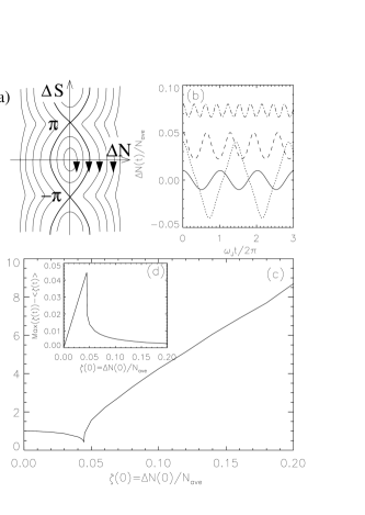
Figure 5: Dynamics of two identical fragment system: (a) Flow diagram in the phase space. (b) Time evolution of the density variation with different initial $\Delta N$. (c) Oscillation frequency and (d) amplitude (about its average value) as a function of initial density modulation from equilibrium value.

In such simple two-fragment situation, an interesting phenomenon, “self-trapping” effect can be observed in the two-fragment case when $\Delta S$ is larger than $\pi$. As shown in the phase portrait of Fig. 5(a), the system trajectories of the initial conditions denoted by the first two right arrows do not pass the origin ($\Delta N=0$) and keep flow away by growing $\Delta S$ exponentially. In Fig. 5(b), we show a numerical results for $\Delta N(t)$ from different initial $\Delta N(0)$ (with $\Delta S(0)=0$), using a set of typical parameters: $N_{1}^{0}=N_{2}^{0}=10^{5}$, $K_{1,2}=1$ Hz and $\bar{U}=0.05$ Hz. We can see that when initial displacement, $\Delta N(0)/N_{1}$, is less than 1% (solid line), the number of atoms oscillates between these two fragments with frequency $\omega_{J}=100$ Hz. When $\Delta N(0)$ increases, the oscillation amplitude first increases accordingly (dotted line) and then suddenly decreases for $\Delta N(0)>\Delta N_{c}\sim 0.04N_{1}$ (dashed and dash-dotted lines). Besides, the density imbalance $\Delta N(t)$ then never passes zero but just oscillates about a new average value. Such counterintuitive result is due to the nonlinear nature of Eq. (34), and can be realized in a single pendulum problem where the weight has a very large initial velocity to overcome the gravitation potential even at the highest position of the circle ($\Delta S=\pi$) and then keep rotating forward with a nonzero velocity (see the trajectory following the first two right arrow in Fig. 5(a)). It is also very similar to the Ac Josephson effect, where a constant electric potential drop between the two connecting superconductors can cause a oscillating current between them. In our present situation, the initial potential drop is provided by the large imbalance of number of particles so that the fast oscillation of single particle tunneling cannot reduce such initial imbalance except for other damping mechanism. We can calculate the critical amplitude of the initial density variation easily and obtain

$$|\Delta N_{c}|=2\sqrt{\frac{2\tilde{K}}{\bar{U}}}.$$ (36)

We note that such critical density variation becomes smaller when the tunneling energy is weaker and/or the average onsite charging energy is larger, i.e. close to the insulating phase.

In Fig. 5(c)-(d), we plot the oscillation frequency and amplitude as a function of different initial density variation, $\zeta(0)=\Delta N(0)/N_{\rm ave}$. It is easy to see that the oscillation amplitude drops very fast when initial displacement is larger than the self-trapping point. This result also exists even when considering the full quantum mechanics in such simple two well system anatoli , because the typical number of particles per site in the fragments is so large ($>10^{4}$) that the quantum fluctuation can be neglected.

III.4 Shaking experiment in condensate fragments

In optical lattice system, the dynamics of a condensate cloud can be studied by the “shaking experiment”, a suddenly shifting of the global confinement potential with a finite displacement, and then observing the successive center of mass motion bishop ; shaking_exp . When the initial displace is small, the condensate oscillates harmonically, showing a coherent Josephson junction tunneling between neighboring wells. When the displacement is larger than some critical value, however, the center of mass motion becomes strongly damped, indicating a dynamical instability, which is a classical phase transition due to the breakdown of meanfield solution bishop . It is believed that when the strength of optical lattice is tuned to be strong enough, the shaking experiment with small displacement can be used to investigate the proposed superfluid to (Mott) insulator transition zoller ; SF-MI , where (unlike in the superfluid phase) the small displacement should not result in a coherent center of mass motion anatoli_dw . In our earlier work early_work , we proposed that similar experiments can be done to investigate the superfluid to insulator transition in the microchip fragments, where the insulating phase is best understood as a Bose glass phase due to the underlying disorder nature bose_glass . Here we will study such multi-well dynamics in more details via the meanfield equation of motion derived in Eqs. (34)-(35).

However, although there are many similarity between the condensate fragments we consider here and the condensates in optical lattice zoller ; optical_lattice ; bose_glass , their difference in the sizes of local potential wells does bring some significant difference of their dynamics. We first note that due to the large size of the disorder potential well in the microchip, the overall condensate density profile is far away from the result of Thomas-Fermi inverse paraba (compared the solid and dotted lines in Fig. 3(b)). Actually, one can expect that the density profile has a kind of “discontinuity” around the edge of the whole condensate. Applying the self-trapping dynamics discussed in previous section, we then expect that the atoms in the edge fragments will not effective tunneling into the potential well next to it, which is created by shifting the confinement potential (see Fig. 6(a)). Such strong edge effects is right due to the nonlinearity-induced self-trapping phenomena as discussed earlier. Therefore we do not expect that the condensate fragments will be driven to motion as a whole by such shaking experiment. The only possible exception is by thermalizing the atoms in the edge fragments to higher energy modes, which is certainly not a coherent motion at all and is not our current interest in this paper.

 

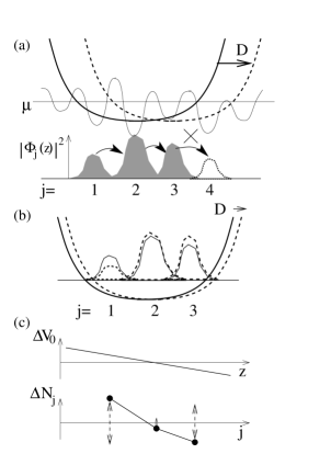
Figure 6: Schematic potential and density profile of condensate fragments in a microchip system. (a) Self-trapping effects for large displacement, $D$. The atoms in fragment 3 cannot tunneling as a condensate into the potential well 4, which is generated by the large displacement of global confinement potential. The noisy curve in the upper portion denotes the local disorder potential, and the lower portion shows the fragment density profile before shaking. Solid/dashed lines denote the global confinement potential before/after shaking. (b) Density variation for small displacement (no disorder potential is shown here).The dashed line for the density profile denotes the new equilibrium profile in the new potential after shaking. Solid lines are the density profile before shaking. (c) The potential and density variation with respect to the new potential and equilibrium density profile. Such $\Delta N_{j}$ becomes the source of fragment dynamics as time evolves. Up-down arrows indicate the possible density oscillation in each well.

Despite of such huge difference, the shaking experiment with small displacement can be still applied to study the coherent motion in the condensate fragments by realizing the density profiles of the whole condensate. As schematically shown in Fig. 6(b), although the small displacement $D$ may not change the whole condensate position with respect to the disorder potential, it is indeed capable to change the onsite potential strength to a slightly new value, and hence the atoms in each fragments become to flow between neighboring wells to response the change of local chemical potential. Precisely speaking, such small displacement shift should change the shape of local potential well also, and hence change their position as well as well width/depth. However, we believe it is a reasonable approximation to neglect the change of well positions and widths, and concentrate on the effects mainly from the deviation of local chemical potential, which gives a new equilibrium density profile, $N_{j}^{new}$, so that the old density profile, $N_{j}^{old}$, becomes an initial non-equilibrium source for the coming dynamics. In Fig. 6(c), we schematically depict the linear change of (parabolic) confinement potential and hence the unbalanced density source for the future dynamics, $\Delta N_{j}\equiv N_{j}^{old}-N_{j}^{new}$. If the whole condensate is in superfluid regime, we expect that $\Delta N_{j}(t)\equiv N_{j}(t)-N_{j}^{new}$ will oscillate about zero with a definitely phase relation with respect to its neighboring site (vertical dashed arrows in Fig. 6(c)), when $|\Delta N_{j}(t)|$ is small enough. In general, the density variation ($\zeta_{j}(t)\equiv|N_{j}(t)-N_{j}^{0}|/N_{j}^{0}$, where $N_{j}^{0}\equiv N_{j}^{new}$ and $N_{j}(t=0)=N_{j}^{old}$) is largest at the edge fragments, because the potential deviation is the largest there while its average number of atoms ($N_{j}^{0}$) is in general smaller than the fragments in the center of condensate.

In the following calculation of fragment dynamics, we shift the constant change of chemical potential so that $\Delta V_{0}(z)=\frac{m}{2}\omega_{\|}^{2}(z+D)^{2}-\frac{m}{2}\omega_{\|}^{2}z^{2}=m\omega_{\|}^{2}Dz\equiv{\cal D}z$ is zero at the center of the whole condensate with an effective potential displacement ${\cal D}$. The initial density variation (i.e. the density before shaking, $N_{j}^{old}$, respect to the new equilibrium density, $N_{j}^{new}$, after shaking) can be approximated by $\Delta N_{j}(t=0)\sim\Delta V_{0}(z_{j})/U_{j}$. We will therefore consider how the density variation ($\Delta N_{j}(t)$) evolves as a function of time with different displacement, ${\cal D}$. Besides, we also make a further approximation by assuming the global confinement potential can be neglected when calculating the onsite wavefunction and other dynamical variables, because they are mainly determined by the local disorder potential.

III.5 Numerical results

As an example of the condensate fragment dynamics, we show in Fig. 7 the typical results for a four fragment system. We choose $K_{1,2}=K_{3,4}=1$ Hz $K_{2,3}=0.5$ Hz, $U_{1,2,3}=0.05$ Hz, and $N_{1}^{0}=N_{4}^{0}=1.3\times 10^{5}$ and $N_{2}^{0}=N_{3}^{0}=1.2\times 10^{5}$ as some typical values shown in Section III.2. Several features can be observed from Fig. 7. (i) When the displacement is small (solid lines), both density profiles and phase gradients oscillate about their new equilibrium values with small amplitude. (ii) When the displacement is increased, one of the phase gradient (here it is $S_{3}-S_{2}$) becomes unbound, leading to a self-trapping phenomena where the density profile oscillates around a nonzero mean value (dashed lines). (iii) Between the generic oscillation in small displacement and the self-trapping in the large displacement, we find that the condensate dynamics becomes chaotic in the intermediate range of displacement (dotted lines). Such chaotic dynamics can be investigated via the frequency spectrum (see Ref. [early_work, ]) or the time correlation function. This is a classical instability of the meanfield GPE, and its result to the center of mass motion in optical lattice has been investigated in Refs. [bishop, ].

 

Figure 7: (a) Density and (b) phase oscillation in each fragments of a typical four fragment condensate. In both figures, solid, dotted, and dashed lines are results for $\cal D$=0.15, 0.2, and 0.3 Hz/$\mu$m respectively. In (a) the four sets of curves are for well $j=1$, 2, 3, and 4 respectively from bottom to top. In (b) the three sets of curves are phase gradients in the neighboring sites: $S_{2}-S_{1}$, $S_{3}-S_{2}$, and $S_{4}-S_{3}$ respectively from bottom to top.

In Fig. 8 we plot a numerical calculated dynamical phase diagram for ten-fragment system with $N_{tot}=2\times 10^{6}$ sodium atoms in the disorder potential calculated earlier (at $d=100$ $\mu$m) in terms of disorder strength ($s$) and critical displacement, $D$. Here the dashed line separates the multi-mode oscillation (e.g. solid lines in Fig. 7) from the chaotic motion (e.g. dotted lines in Fig. 7), while the solid line separates the multi-mode/chaotic motion from the self-trapping motion (e.g. dashed lines in Fig. 7). We can see that the critical displacement of self-trapping decreases dramatically for $s=u_{s}/u_{s}^{0}<1.1$ and then becomes smoothly for $s>1.1$. It never reaches zero in our meanfield approximation. We believe that after including the full quantum fluctuation, the meanfield solution becomes incorrect in the strong disorder region, where the quantum fluctuation can decrease the critical displacement so much that even infinitesmall displacement to the condensate will be self-trapped without coherent motion (i.e. the solid line of Fig. 8 terminates at finite disorder strength, say $s=1.1$) anatoli_dw . This can be understand as a signature of quantum phase transition from superfluid phase in small disorder to an insulating phase in strong disorder, which is best understood as a Bose glass phase fisher due to the nature of randomness. However, since the low energy excitation properties in such strong disorder regime are still poorly understood, we could not exclude the possibility of different quantum phases, such as Mott glass as suggested by Giamarchi et. al. giamarchi_mott due to the competition between a (white noise) random potential and a commensurate periodic potential.

 

Figure 8: Critical shaking displacement of a ten-fragment system as a function of disorder strength ($s=u_{s}/u_{s}^{0}$). Total number of atoms is $2\times 10^{6}$.

 

Figure 9: The dotted line shows the probability P($Q<1$). The system is in the superfluid state when this probability is close to zero (see text), while it is in an insulating state when it is close to one. The solid line shows the probability that one can observe fluctuations in the number of atoms between the neighboring wells with fluctuations in the number of particles larger than $\zeta_{\rm min}=0.1$ and oscillation frequency larger than $\omega_{\rm min}=2\pi\times 1$ Hz. When this probabilities approaches zero, the system will appear self-trapped in the shaking experiments. Here $N_{\rm ave}$ is the average number of atoms in a single well (mini-condensate). Disorder strength for (a) are the same as used in Fig. 3b for $d=100$ $\mu$m (denoted to be $u_{s}^{0}$), while it is five times stronger in (b). The results are averaged over more than twenty thousand pairs of two-fragment system with average number of atoms, $N_{\rm ave}$, per well.

III.6 Estimate quantum fluctuation effects

The transition from superfluid phase to insulator phase is driven by the quantum fluctuation in the competition between interaction and random potential fisher . Including the quantum fluctuations in the dynamics of condensates has been studied in some limited cases qt_dynamics ; qt_dynamics2 by either solving the full coupled nonlinear Gross-Pitaevskii-Bogoliubov-de-Gennie equation qt_dynamics , using dynamical meanfield variational method zoller or by using truncated Wigner approximation qt_dynamics2 . Studies including random potential is much more difficult and still in progress. Here we will give some estimate about such transition using the statistical properties, which, at least in principle, should be able to be probed by the dynamical shaking experiment when displacement is tuned to infinitesmall.

Transition into the insulating state may be characterized by the ratio of the “Josephson energy” between the neighboring wells to the charging energy of one of the wells, i.e. $Q_{j}\equiv\frac{8{K}_{j,j+1}N_{j}^{0}N_{j+1}^{0}}{(U_{j}+U_{j+1})/2}$. Without disorder potential, the meanfield calculation ehud ; sachdev estimates the superfluid (SF) to Mott insulator (MI) transition at $Q=1$. For the Gaussian correlated random potential we discuss here, we expect that quantum fluctuation induced SF to BG phase transition note2 should also appear at roughly the same place. Due to the randomness nature of the condensate fragments, the effects of quantum fluctuation is important if the probability to have $Q_{j}<1$ ($\equiv{\cal P}(Q<1)$), is of the order of one, where the probability if obtained by averaging over disorder ensemble. In Fig. 9 we show the calculated ${\cal P}(Q<1)$ as a function of the atom density for two different strengths of the disorder potential (dotted lines). In order to capture the quantum fluctuation nature of each random junction, we calculate $Q$ for each pair of fragments across the potential barrier with average number of atoms $N_{\rm ave}$ per well. According to Fig. 9, we can estimate that the quantum fluctuations are crucially important to a pair of fragments when $N_{\rm ave}<10^{4.4}\sim 2.5\times 10^{4}$ for $s=u_{s}/u_{s}^{0}=1$. This critical average number of particles become higher ($N_{\rm ave}<10^{5}$) for stronger disorder potential ($s=u_{s}/u_{s}^{0}=5$). In the same figure, we also show the calculated probability (solid lines) to have Josephson frequencies $\omega_{J}$ to be larger than some minimum frequency, $\omega_{\rm min}=2\pi\times 1$ Hz, and the density contrast, $\zeta=\frac{\Delta N}{N_{0}}$, to be larger than $\zeta_{\rm min}=10\%$. The values of $\omega_{\rm min}$ and $\zeta_{\rm min}$ are given by the experimental resolution of frequency and density deviations private for the density oscillation. We can see that this probability (denoted by ${\cal P}(\omega>\omega_{\rm min},\zeta>\zeta_{\rm min})$) decreases when average number of atoms per well decreases and/or the disorder strength increases (toward the insulating phase). Both of these two results (${\cal P}(Q<1)$ and ${\cal P}(\omega>\omega_{\rm min},\zeta>\zeta_{\rm min})$) suggest that one can observe the superfluid to insulator (Bose glass) transition note2 in the parameter regime of present experiments.

It is interesting to compare above estimate of quantum fluctuations (Fig. 9) with the dynamical phase diagram associate with the shaking experiments shown in Fig. 8. In Fig. 8, the dynamical properties are calculated for an ensemble of ten fragments, instead of two. Since the superfluid dynamics of the whole condensate can be strongly suppressed if one of these junctions (say, junction $l$ between fragment $l$ and $l+1$) becomes insulating due to strong quantum fluctuation ($Q_{l}<1$), we can roughly estimate that the criterion of superfluid to insulator transition occurs when $M_{\rm junc}{\cal P}(Q<1)$ is of order of one, where $M_{\rm junc}$ is number of total junctions. From the data shown in Fig. 9(a), we can see that this value is about $9\times 0.05=0.45$, for $N_{\rm ave}\sim\log(2\times 10^{5})=5.3$. Therefore we find that the quantum fluctuations of a ten-fragment condensate with $N_{\rm ave}\sim 2\times 10^{5}$ per well should become strong when the disorder strength is about (or slightly larger than) $u_{s}^{0}$. This is consistent with the estimate (see previous subsection) via the self-trapping phenomena observed in a meanfield dynamics associate with shaking experiments shown in Fig. 8.

Finally we note that the results shown in Fig. 9(b) are obtained by the same effective 1D interaction strength used in Fig. 9(a). In the realistic experiment, however, $g_{\rm 1D}$ will be changed if one tunes the wire current and the bias field, $B_{\perp}$ simultaneously (in order to keep condensate at the same position). This is because the effective radial confinement energy will be also increased during such process. However, it is easy to show that one can reduce the confinement energy effectively by increasing the off-set magnetic field, $B_{\|}$, simultaneously without changing any other system parameters. Therefore the final system can be kept almost the same as the one before tuning, except the disorder field has been increased or decreased independently via the composed process mentioned above.

IV Finite temperature effects

To estimate the validity of our calculation in finite temperature regime, we take the following four steps: (i) first we have to clarify the general concept about the temperature effects in low dimensional BEC system. (We do not need to include any disorder potential at this point.) Due to the finite size effects in the longitudinal direction, it is possible that a boson system becomes 1D quantum degenerate (or say the lowest energy eigenstate becomes macroscopically occupied, see Ref. [ketterle, ]) when the temperature is below the degeneracy temperature, $T_{d}=N\omega_{\|}/\ln(2N)$, where $N$ is the total number of atoms and $\omega_{\|}$ is the confinement frequency in the longitudinal direction. When considering the interaction-induced thermal phase fluctuation effects for temperature below $T_{d}$, Petrov et. al. petrov show that a true condensate, where both density and phase fluctuations are small within the finite system size, can be achieved when temperature is below another temperature scale, $T_{ph}=T_{d}\times\omega_{\|}/\mu$, where $\mu$ is the chemical potential. For a temperature between these two temperatures, i.e. $T_{ph}<T<T_{d}$, the system has a frozen density fluctuation but finite thermal phase fluctuation. The typical experimental parameters (as we consider in this paper in a superfluid regime), we can estimate that $T_{d}\sim 13.2$ $\mu$K, and $T_{ph}\sim 127$ nK (for $N=10^{6}$, $\omega_{\|}=2\pi\times 4$ Hz, and that chemical potential is about 3 kHz for atom-wire separation being about 100 $\mu$m). The present experiments were done at a temperature of about 100 nK private . Therefore, we can safely say that the condensate we consider here (similar to the present experimental conditions of MIT group) is in the true condensate regime (or deep in the quasi-condensate regime), where thermal fluctuation is very small or the thermal fluctuation length is comparable to the whole system size.

(ii) Secondly, we consider the presence of a strong disorder potential, where we approximate the fragmented condensate by a single band Bose-Hubbard model and solve its dynamics in meanfield approximation. The first approximation can be easily justified in our system from the following two reasons: first, we can turn on the disorder potential (by moving the atom cloud closer to the wire) adiabatically, so that the ground state remains in condensate without high-energy excitations. Actually, the effective temperature compared to the band gap becomes even smaller due to the shrink of band energy, since no thermal reservoir is connected to the atom cloud trapped in the magnetic field (thermal fluctuation from the wire surface henkel can be neglected here because of the larger atom-wire separation). This is very similar to the situation in an optical lattice. Secondly, each fragment itself is in the true condensate regime due to large number of atoms ($\sim 10^{4-5}$) and stronger confinement provided by the correlated disorder potential. The critical temperature estimated for a single fragment is about $T_{ph}\sim 1$ $\mu$K, well above the temperature quoted in the experiments. Therefore, the thermal excitation to a higher energy band is strongly suppressed and can be safely neglected.

(iii) However, the second approximation, the meanfield approximation for the dynamical motion of condensates, is self-justified only when in the deep superfluid regime and when the temperature is lower than both the Josephson energy $\tilde{K}_{j,j^{\prime}}$ and the local chemical potential deviation, $\delta\mu=U_{j}(N_{j}-N_{j}^{0})$ (see Eqs. (34)-(35)), which are the only two energy parameters in a meanfield version of the Hubbard model. Using the typical parameters we tracked from the data of the MIT group, the above criteria can be safely fulfilled due to the large number of atoms per fragment.

(iv) Finally, we apply such a single band Hubbard model to study the quantum phase transition by increasing the disorder potential strength (Fig. 8) or by reducing the number of atoms per well (Fig. 9). When considering the quantum fluctuation effects near the transition point, we note that the temperature has to be below the charging energy, $U_{j}$, instead of $N_{j}U_{j}$ in the classical limit, in order to see the quantum effects. Such a condition, however, may not be satisfied in our system. In other words, the finite temperature effects may smoothen the transition/crossover from the superfluid phase to the insulating Bose glass phase, but such crossover should still be controlled by the zero temperature quantum critical point. Therefore, we believe our results, like Fig. 9 and dynamical properties near the insulating phase, should still be qualitatively valid at finite temperature.

V Summary

In summary, we study in detail the disorder magnetic potential in an atomic waveguide (microchip) and quantitatively explain the fragmentation phenomena observed in the experiments. Our results shows that the disorder effects can be very strong even for a very small wire edge fluctuation, and hence not negligible in most of the present experimental situations. We also study the dynamical properties of an array of fragments (self-trapping, multi-pole oscillation and modulational instability), and propose a superfluid-to-insulator crossover in strong disorder limit, which can be probed by a shaking experiment within the experimentally accessible regime.

VI Acknowledgement

The authors thank useful discussion with E. Demler, A.E. Leanhardt, S. Kraft, L.D. Lukin, D.E. Pritchard, G. Rafel, E. Altman, and W. Hofstetter. We especially acknowledge the critical discussion with A.E. Leanhardt for the experimental details.

References

- (1) W. Ketterle and N.J. van Druten, Phys. Rev. A 54, 656 (1996).
- (2) D.S. Petrov, et. al., Phys. Rev. Lett. 85, 3745 (2000); ibid. 87, 050404 (2001); U. Al Khawaja, J.O. Andersen, N.P. Proukakis and H.T.C. Stoof, Phys. Rev. Lett. 88, 070407 (2002).
- (3) J.O. Andersen, U. Al Khawaja, and H.T.C. Stoof, Phys. Rev. Lett. 88, 070407 (2002).
- (4) W. Hansel, et. al., Nature 413 498 (2001); J.H. Thywissen, et. al., Eur. Phys. J. D. 7, 361 (1999); R. Folman, et. al., Adv. At. Mol. Opt. Phys. 48, 263 (2002).
- (5) A.E. Leanhardt, et. al., Phys. Rev. Lett. 89, 040401 (2002).
- (6) D. Cassettari, et al., quant-ph/0003135. T. Schumm, et al., Nature Phys. 1, 57 (2005).
- (7) K.K. Das, M.D. Girardeau, and E.M. Wright, Phys. Rev. Lett. 89, 170404 (2002); K.K. Das, G.J. Lapeyre, and E.M. Wright, Phys. Rev. A 65, 63603 (2002).
- (8) L. Tonks, Phys. Rev. 50, 955 (1936); V. Dunjko, V. Lorent, and M. Olshanii, Phys. Rev. Lett. 86, 5413 (2001); M.D. Girardeau and E.M. Wright, Phys. Rev. Lett. 87, 210401 (2001).
- (9) A.E. Leanhardt, private communication.
- (10) A.E. Leanhardt, et. al., Phys. Rev. Lett. 90, 100404 (2003).
- (11) J. Fortagh, et. al., Phys. Rev. A 66 041604 (2002).
- (12) S. Kraft, et. al., J. Phys. B, 35, L469 (2002).
- (13) M.P.A. Jones, C.J. Vale, D. Sahagun, B.V. Hall, C.C. Eberlein, B.E. Sauer, K. Furusawa, D. Richardson, E. A. Hinds, cond-mat/0308434 (unpublished).
- (14) T. Paul, P. Leboeuf, N. Pavloff, K. Richter, and P. Schlagheck, Phys. Rev. A 72, 063621 (2005).
- (15) K. Huang and H. F. Meng, Phys. Rev. Lett. 69, 644 (1992).
- (16) S. Giorgini, L. Pitaevskii, and S. Stringari, Phys. Rev. B 49, 12938 (1994).
- (17) A.V. Lopatin and V.M. Vinokur, PRL 88, 235503 (2002).
- (18) U. C. Tauber and D. R. Nelson, Phys. Rep. 289, 157 (1997).
- (19) T. Giamarchi and H. Schulz, Phys. Rev. B 37, 325 (1988).
- (20) M.P.A. Fisher, et. al. Phys. Rev. B, 40, 546 (1989).
- (21) J.D. Reppy, J. Low. Temp. Phys. 87, 205 (1992); P.A. Crowell, et. al., Phys. Rev. B 51, 12721 (1995).
- (22) B. Damski, J. Zakrzewski, L. Santos, P. Zoller, and M. Lewenstein, Phys. Rev. Lett. 91, 080403 (2003).
- (23) J. E. Lye, L. Fallani, M. Modugno, D. S. Wiersma, C. Fort, and M. Inguscio, Phys. Rev. Lett. 95, 070401 (2005); T. Schulte, S. Drenkelforth, J. Kruse, W. Ertmer, J. Arlt, K. Sacha, J. Zakrzewski, and M. Lewenstein, Phys. Rev. Lett. 95, 170411 (2005).
- (24) L. Fallani, J. E. Lye, V. Guarrera, C. Fort, and M. Inguscio, cond-mat/0603655.
- (25) D.-W. Wang, M.D. Lukin, and E. Demler, Phys. Rev. Lett. 92, 076802 (2004).
- (26) C. Hankel and S. Gardiner in cond-mat/0212415, C. Hankel, S. Potting, and M. Wilkens, Appl. Phys. B 69, 379 (1999). M.P.A. Jones, et. al., cond-mat/0301018.
- (27) J. Esteve, C. Aussibal, T. Schumm, C. Figl, D. Mailly, I. Bouchoule, C. Westbrook, and A. Aspect, Phys. Rev. A, 70, 043629 (2004).
- (28) T. Schumm, J. Esteve, C. Aussibal, C. Figl, J.-B. Trebbia, H. Nguyen, D. Mailly, I. Bouchoule, C. Westbrook, and A. Aspect, Euro. Phys. J D 32, 171 (2005).
- (29) C.J. Penthick, and H. Smith, Bose-Einstein Condensation in Dilute Gases (Cambridge, New York, 2002).
- (30) We note that in principle, one should solve the 3D Gross-Pitaevskii equation (GPE) for the enlongated trap potential, , in the presence of disorder potential, to obtain the 3D condensate density profile, and then integrate out the transverse dimensions to get the one-dimensional density profile to compare with the experimental data. However, in above calculation we approximate such 3D calculation by the 1D meanfield Gross-Pitaevskii equation for simplicity, where the transverse mode is assumed to be in the gaussian lowest ground state and the whole transverse confinement effects are absorbed into the effective scattering amplitude, . Such approximation is valid if , where is average 1D density. In the soldium system of MIT group we consider above, (for m) is just above order of one. Therefore only few (not many) transverse modes are occupied, which should not be well-described either by 3D meanfield (good for ) or by 1D meanfield (good for ). But since we are interested in strong confinement limit in all of our systems (but not so strong to Tonks gas limit), we think the 1D meanfield approximation is still an appropraite approximation.
- (31) D. Jaksch, et. al., Phys. Rev. Lett. 81, 3108 (1998).
- (32) E. Altman, Y. Kafri, A. Polkovnikov, G. Refael, Phys. Rev. Lett. 93, 150402 (2004).
- (33) See for example, M. Tinkham, Introduction to Superconductivity (McGraw Hill, New York, 1996).
- (34) A. Polkovnikov, S. Sachdev, and S.M. Girvin, Phys. Rev. A 66, 53607 (2002).
- (35) A. Smerzi, et. al. Phys. Rev. Lett. 89, 170402 (2002); F.S. Cataliotti, et. al., New J. Phy. 5, 71.1 (2003).
- (36) F.S. Cataliotti, Science 293, 843 (2001).
- (37) papers for superfluid-to-Mott insulator transition.
- (38) A. Polkovnikov and D.-W. Wang, Phys. Rev. Lett. 93, 070401 (2004).
- (39) T. Giamarchi, P. Le Doussal and E. Orignac, Phys. Rev. B 64, 245119 (2001).
- (40) Y. Castin and R. Dum, Phys. Rev. Lett. 79, 3553 (1997).
- (41) A. Sinatra, C. Lobo, and Y. Castin, Phys. Rev. Lett. 87, 210404 (1997); A. Polkovnikov, Phys. Rev. A, 68, 033609 (2003); A. Polkovnikov, Phys. Rev. A, 68, 053604 (2003).
- (42) E. Altman, and A. Auerbach, Phys. Rev. Lett. 89, 250404 (2002).
- (43) S. Sachdev. Quantum Phase Transitions (Cambridge, New Tork, 1999).
- (44) Note that in the thermodynamic limit, various regimes may be distinguished only for a bounded disorder, while in a finite system there is no true phase transition — however, one may still observe the sharp crossovers.