Are better conducting molecules more rigid?

Abstract

We investigate the electronic origin of the bending stiffness of conducting molecules. It is found that the bending stiffness associated with electronic motion, which we refer to as electro-stiffness, $\kappa_{e}$, is governed by the molecular orbital overlap $t$ and the gap width $u$ between HOMO and LUMO levels , and behaves as $\kappa_{e}\sim t^{2}/\sqrt{u^{2}+t^{2}}$. To study the effect of doping, we analyze the electron filling-fraction dependence on $\kappa_{e}$ and show that doped molecules are more flexible. In addition, to estimate the contribution of $\kappa_{e}$ to the total stiffness, we consider molecules under a voltage bias, and study the length contraction ratio as a function of the voltage. The molecules are shown to be contracted or dilated, with $\kappa_{e}$ increasing nonlinearly with the applied bias.

Conducting polymers have been extensively studied over the last decades because of their vast electronic device applications. They have $\pi$-orbital overlapping along a conjugated backbone and a gap between the highest filled and the lowest unfilled bands, forming a band structure similar to inorganic semiconductors. When an electron is removed or added, the conductivity is greatly enhanced, allowing these semiconductors to be utilized as organic electronic device. On the other hand, conducting polymers are much more flexible than semiconducting solids, while their electronic functions are very similar. This property has led to studies for exploring their mechanical deformations such as bending and expansion/contraction driven by electric triggering. It is known that the oxidation causes the expansion or the contraction of conducting polymers, depending on whether ions are inserted or eliminated kaneto1 . Also, chemical doping drives electromechanical deformation by delocalizing the $\pi$-electrons kaneto2 ; watanabe .

The structural stiffness of a material is determined by many factors, such as atomic binding energies, the nature of molecular bonding, inter-polymer adhesion, to mention a few. It is worthwhile to note that the orbital stack would be an additional source for mechanical rigidity, because in order to achieve better electronic conduction, structural deformations leading to a loss in orbital overlap are less favored. Despite this great diversity of causes for the mechanical stiffness of materials, in this work, we present the first step to relate electronic properties of these materials with their mechanical stiffness. This is essential not only to relate the electronic origin of stiffness with chemistry-based factors but also to grasp the mechanical response to electric signal which differs from polymer to polymer. For instance, the extension ratio of Polyalkylthiophene (PAT) is larger than that of Polypyrrole (PPy) kaneto . It is interesting to relate it to the difference in their electronic band structures. Although they have comparable orbital overlap, the gap between HOMO and LUMO levels in PAT is about half of that in PPy hutchison . This indicates that not only orbital overlap but also band gap comes into play for mechanical stiffness.

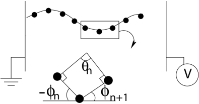
Figure 1: Schematic picture of a conducting polymer between two electrodes. The one with the anchored polymer is grounded and the other is fixed at voltage $V$. The polymer configurations are discretized in a way such that the bond angle and the mean position of two adjacent beads define the tangential angle $\phi_{n}$ and position of $n$th monomer, respectively.

In this work, we investigate the effect of the electronic properties of conducting polymers on their conformational stiffness. This enables us to understand mechanical responses as well as to estimate the electronic contribution to the total structural rigidity. For this purpose, we model conducting polymers as a one-dimensional chain composed of $N$-monomer where inter-monomer hopping of electrons is allowed via $\pi$-orbital stacking. More specifically, to investigate the bending rigidity, we assume the hopping strength to depend on the angular configuration of monomers Hone . Furthermore, to simulate the HOMO-LUMO gap, an alternating on-site potential is included in the Hamiltonian. Following a semi-classical approach, we trace over the electronic degree of freedom and obtain the effective potential for the angle deformations. We find that the bending stiffness associated with electronic properties, which we refer to as electro-stiffness, $\kappa_{e}$, is governed by the molecular orbital, $t$ and gap width between HOMO and LUMO level, $u$, and scales as $\kappa_{e}\sim t^{2}/\sqrt{u^{2}+t^{2}}$. Further by analyzing the electron-filling fraction dependence on $\kappa_{e}$, we show that doping would make the molecules more flexible. To evaluate the specific contribution of $\kappa_{e}$ to the total rigidity, we consider molecules under a voltage bias and examine the length contraction as a function of the bias. It turns out that the applied voltage alters the electro-stiffness, resulting in the length contraction (dilation) of the molecules.

We consider a conducting molecule in the presence of an external electric field. The Hamiltonian for the electrons responsible for the conducting behavior is taken as

$${\cal H}_{e}=-\sum_{n}t_{n,n+1}(c_{n}^{\dagger}c_{n+1}+\mbox{h.c})+\sum_{n}[(-1)^{n}u-vx_{n}]c^{\dagger}_{n}c_{n}.$$ (1)

Here the inter-site hopping integral $t_{n,n+1}$ is determined by the degree of $\pi$-orbital overlap, and is maximum when the molecule is in a straight form. When the molecule is not in the straight conformation, the overlap is decreased, which tends to suppress electron hopping. We incorporate this fact by introducing an angle-dependence in the hopping integral as $t_{n,n+1}=t\cos(\phi_{n+1}-\phi_{n})\equiv t\cos\theta_{n}$. For $\theta_{n}=0$, the hopping parameter is spatially uniform and maximized by parallel orbital arrangement. In the second term we introduce an alternating on-site potential, yielding a gap whose width is determined by $u$. This enables us to investigate semiconducting molecule having a gap between HOMO and LUMO level. Also, the on-site potential is position dependent due to the applied voltage $V$ and $v=|e|Va/L$ is the voltage drop across one monomer with electrode spacing $L$(see Fig. 1). Taking the monomer spacing as $a$, we write $x_{n}=\sum_{i=0}^{n}\cos\phi_{i}-(1/2)\cos\phi_{n}$.

The Hamiltonian contains several electronic factors that contribute to the structural rigidity: (i)the electron hopping favored by a straight configuration; (ii)the band gap making the molecules less conducting and tending to diminish the effect of the factor (i); (iii) the applied voltage bias inducing length contraction or extension. The rigidity from electronic origin, $\kappa_{e,n}$, can be obtained by

$$\kappa_{e,n}=-\frac{k_{B}T}{2}\frac{\partial^{2}}{\partial\theta_{n}^{2}}\ln\mbox{Tr}_{\{c,c^{\dagger}\}}\exp(-\beta{\cal H}_{e}),$$ (2)

which can be site-dependent when boundary effects are considered. In fact, the rigidity also has contributions from molecular bonding and atomic binding potentials, which we denote as $\kappa_{m}$, and the potential governing the structural rigidity is written as

$${\cal H}_{m}=\sum_{n}\kappa_{n}\theta_{n}^{2},$$

where $\kappa_{n}=\kappa_{e,n}+\kappa_{m}$. Before proceeding to the numerical evaluation of Eq. (2), we study the small bending of the molecules in the absence of a voltage drop. Expanding the angle to quadratic order, we define

$${\cal H}_{e}^{(0)} = -t\sum_{n}(c_{n}^{\dagger}c_{n+1}+\mbox{h.c})+u\sum_{n}(-1)^{n}c_{n}^{\dagger}c_{n}$$ (3)

$${\cal H}_{e}^{(1)} = \frac{t}{2}\sum_{n}\theta_{n}^{2}(c_{n}^{\dagger}c_{n+1}+\mbox{h.c}),$$

where the position of the $n$th monomer for small $\phi$’s is denoted by $x_{n}$. Assuming ${\cal H}_{e}^{(1)}$ to be a small perturbation, we can write $-k_{B}T\ln\langle e^{-\beta{\cal H}_{e}^{(1)}}\rangle_{0}\approx\langle{\cal H}_{e}^{(1)}\rangle_{0}$, where $\langle X\rangle_{0}={\cal Z}_{0}^{-1}\mbox{Tr}Xe^{-\beta{\cal H}_{e}^{(0)}}$ with ${\cal Z}_{0}=\mbox{Tr}e^{-\beta{\cal H}_{e}^{(0)}}$. It is convenient to work in the Fourier space: $c_{n}=N^{-1/2}\sum_{n}e^{ikn}c_{k}$. The Hamiltonian ${\cal H}_{e}^{(0)}$ can then be straightforwardly diagonalized by the canonical transformation $c_{k}=\cos\chi_{k}a_{k,+}+\sin\chi_{k}a_{k,-}$ and $c_{k+\pi}=-\sin\chi_{k}a_{k,+}+\cos\chi_{k}a_{k,-}$ as

$${\cal H}_{e}^{(0)}=\sum_{k,\alpha=\pm}\lambda(k)a_{k,\alpha}^{\dagger}a_{k,\alpha},$$

where $\lambda(k,\alpha)=\alpha\sqrt{\epsilon^{2}(k)+u^{2}}$ with $\epsilon(k)=-2t\cos k$ and $\tan 2\chi_{k}=-u/\epsilon(k)$ and $\alpha=\pm 1$. Similarly we can write ${\cal H}_{e}^{(1)}$ in terms of the diagonalizing basis, with off-diagonal components. In evaluating $\langle{\cal H}_{e}^{(1)}\rangle_{0}$, however, since ${\cal H}_{el}^{(0)}$ is quadratic in the $c$’s, the only non-vanishing contributions can be easily traced and we get

$$\kappa_{e}=\frac{1}{N}\sum_{k,\alpha=\pm 1}\frac{-\epsilon^{2}(k)}{\alpha\sqrt{u^{2}+\epsilon^{2}(k)}}\langle{\cal N}_{k,\alpha}\rangle_{0}$$ (4)

with the mean number of particles occupying the $\alpha=+1$ and $-1$ bands being determined by

$$\langle{\cal N}_{k,\alpha}\rangle_{0}=\langle a^{\dagger}_{k,\alpha}a_{k,\alpha}\rangle_{0}=[e^{\beta(\lambda(k,\alpha)-\mu)}+1]^{-1}.$$ (5)

Figure 2: The electro-stiffness $\kappa_{e}$ vs the hopping integral for $N=40$ in the absence of a voltage bias. The values of $\kappa_{e}$ depend on the monomer position, those near the boundaries, e.g. $n=1$ being smaller than those at $n=N/2$. For a given $n$, $\kappa_{e}$ is estimated for $u=20$ and $u=60$ to show that an increase in the gap width suppresses the stiffness. The energy scales such as $\kappa_{e},t$ and $u$ are measured in units of thermal energy at room temperature, $k_{B}T=0.025$ eV, throughout this paper.

Let us first consider when the system is half-filled so that $\langle{\cal N}_{k,+}\rangle=0$. From Eq. (4), it is clear that as far as the electronic contribution to the bending stiffness is concerned, the hopping integral plays a dominant role: while the denominator in Eq. (4) characterizes the band width, the numerator is proportional to $t^{2}$. On the other hand, for molecules having comparable hopping strengths, those with large band gap would be more flexible. The numerical evaluation of Eq. (2) has been performed and the resulting stiffness is presented in Fig. 2. It is in good agreement with the perturbative result, Eq. (4). While the analytic expression for the stiffness can be easily obtained for an infinitely long polymer, a finite-sized polymer has boundary effects that are characterized by a site-dependent stiffness. As shown in Fig. 2, the stiffness is weaker in the polymer bulk than in the ends, indicating that when a force is applied, the bending of the polymer would be more localized in the bulk rather than being uniform all over.

Figure 3: The stiffness difference $\Delta\kappa_{e}$ vs the electron filling fraction $\gamma$ for N = 40 in the absence of a voltage bias: for a given $n$, $\kappa_{e}$ is estimated for $t=60$, $u=40$ (PPy) and $t=48$, $u=20$ (PAT) to show that the increase of the gap width suppresses the stiffness. The inset shows $\kappa_{e}$ for a DNA molecule with $t=8$, $u=40$. Here $\kappa_{e},t$ and $u$ are in units of thermal energy at room temperature, $k_{B}T=0.025$ eV

.

Even more interesting is the filling factor dependence of $\kappa_{e}$. When hole/particles are introduced in the system, the electrostiffness becomes weaker than that for a half-filled system, as displayed in Fig. 3. We evaluated the stiffness difference $\Delta\kappa_{e}\equiv\kappa_{e}(\gamma)-\kappa_{e}(1/2)$, where $\gamma$ denotes the filling fraction as $\gamma=N_{e}/N$. This is in good agreement with the experimental observation that the bending rigidity of Polyurethane film is enhanced by salt doping watanabe . This becomes obvious from Eq. (4). When the system is half-filled, $\alpha=(+1)$ band would be empty so that in Eq. (4), the contribution to the stiffness is solely due to the $\alpha=(-1)$ band. On the other hand, when holes are doped, the $\alpha=(-1)$ band becomes partially filled, and the corresponding reduction in $\langle{\cal N}_{k,-}\rangle$ results in a decrease of $\kappa_{e}$.

Figure 4: The derivative of the length contraction ratio $\ell$ vs the voltage bias $v$ for various parameter sets. Here $\sigma$ represents the ratio $\sigma=\frac{\kappa_{m}}{\kappa_{e}}$. The inset shows the length contraction ratio $\ell$ vs $v$ for $\sigma=2$. The square symbols and the filled squared symbols represent $t=60,u=40$ and $t=48,u=20$, respectively. Here $\kappa_{e},t$ and $u$ are in units of thermal energy at room temperature, $k_{B}T=0.025$ eV

.

The electrostiffness depends also on the applied electric field which contributes to the energy of the system via a coupling to the charges of the electrons: when $v\ll t$ and $u$, we may approximate the energy due to the field as $E_{f}=-v\sum_{n}x_{n}\langle c_{n}^{\dagger}c_{n}\rangle$. When a positive voltage bias is applied, the molecule increases its length, and hence the effective stiffness increases. For a negative voltage bias, the molecule tends to contract, resulting in the reduction of its stiffness. Investigating the length deformation as a function of the electric field is thus very useful to evaluate the contribution of $\kappa_{e}$ to the total rigidity $\kappa$. As we mentioned earlier, the structural rigidity comes not only from those electronic degrees of freedom but also from the molecular binding potentials. Since for the latter, the deformation is presumably rather insensitive to the applied electric potential, the length deformation caused by the electric field would directly relate the contribution of $\kappa_{e}$ to the total rigidity. To see this more clearly, let us define the length contraction (extension) ratio $\ell$ as

$$\frac{1}{\ell}\equiv 1-\frac{L}{L_{c}}\approx\frac{1}{2}\langle\phi^{2}\rangle$$ (6)

with $L_{c}$ being the contour length of the polymer, and $\langle\phi^{2}\rangle$ being the average angle fluctuation per monomer, given by $\langle\phi^{2}\rangle=\mbox{Tr}_{\{\phi\}}e^{-\beta\mathcal{H}_{m}}\sum_{i}\phi_{i}^{2}/\mbox{Tr}_{\{\phi\}}e^{-\beta\mathcal{H}_{m}}$. Here, disregarding the site-dependence in $\kappa_{e,n}$ (which as we saw is uniform , except for a few boundary sites), and writing $\mathcal{H}_{m}=\sum_{\langle i,j\rangle}\kappa(\phi_{i}-\phi_{j})^{2}$ where $\kappa=\kappa_{m}+\kappa_{e}$ and $\kappa_{m}$ is the bending rigidity due to molecular bonding. It is clear that $\langle\phi^{2}\rangle\propto 1/\kappa$ and hence, $\partial\ell/\partial v$, which is measurable in experiments, would be simply related to the electric-field dependence of $\kappa_{e}$. Evaluating $\ell$ as a function of the voltage bias for molecules having different $\kappa_{m}$, e.g, $\sigma\equiv\kappa_{m}/\kappa_{e}(v=0,2,5)$, we confirm in Fig. 4 that $\partial\ell/\partial v$ is indeed not very sensitive to $\kappa_{m}$. It is also shown that the length contraction ratio increases nonlinearly with $v$ and its derivative with respect to $v$ is positive. This clearly demonstrates the expected feature that the molecules adjust their length to the voltage, allowing for their use as electro-mechanical switches.

In summary, the electronic origin of bending stiffness was investigated. It was shown that the electro-stiffness, $\kappa_{e}$, is governed by the molecular orbital overlap and the gap width between HOMO and LUMO levels: molecules with wider band width are more flexible. The electro-stiffness can be controlled by molecular doping or by applying a voltage bias. Analyzing the electron filling-fraction dependence on $\kappa_{e}$, we showed that doping makes molecules more flexible. In addition, we considered molecules under a voltage bias to extract the $\kappa_{e}$ contribution to the total stiffness. In response to the applied voltage, the molecules are contracted or dilated with a very nonlinear increase of $\kappa_{e}$ with the applied bias.

To conclude this study, we mention the value of $\kappa_{e}$ for a few molecules. For example, DNA has an extremely narrow band width ($\approx 0.01\sim 0.04$ eV) zhang and its electrostiffness is estimated to be roughly just a few $k_{B}T$. It is well-known that the persistence length of ssDNA is about $\ell_{p}\sim 5$nm dnaper , which is related to the bending energy by $\kappa=(\ell_{p}/a)k_{B}T$. Taking the inter-base distance $a=3.4\AA$, $\kappa\approx 14k_{B}T$, showing that the contribution of $\kappa_{e}$ to the stiffness is significant. For a dsDNA $\ell_{p}\approx 50nm$ and hence $\kappa$ is ten times bigger than that for ssDNA dnaper , while the doubling of $\kappa_{e}$ cannot account for the difference. This suggests that among the energetic factors which govern dsDNA bending, the electronic motions via orbital overlap is not as crucial as the electrostatic repulsion between phosphate groups and the helical structured base staking nar . On the other hand, the persistence length of carbon nanotubes (CNT) lies in a macroscopic range $\ell_{p}=0.1\sim 1\mu$m cntper , which shows that the bending rigidity of CNT is hundreds times larger than that of dsDNA. Noting that the orbital overlap is $t\sim 2.5$ eV, and the band gap is small, $u=0\sim 0.5eV$ ijima , we find $\kappa_{e}\approx 10^{2}k_{B}T$, which shows the important contribution of electro-stiffness to the total stiffness of CNT. In addition, the HOMO and LUMO level of PPy and PAT can be simulated by taking $u=1$ eV and $t=1.5$ eV, and $u=0.5$ eV and $t=1.2$ eV, respectively hutchison . This leads to $\kappa_{e}\approx 34k_{B}T$ for PPy, and $\kappa_{e}\approx 28k_{B}T$ for PAT. Although no direct measurement of the bending rigidity of these materials has been made, this goes in the direction of showing that the latter is more responsive than the former kaneto .

References

- (1) K. Kaneto, M. Kaneko and W. Takashima, Jpn. J. Appl. Phys., 34, L837 (1995).
- (2) K. Kaneto, M. Kaneko, Appl. Biochem. and Biotech., 96, 13 (2001).
- (3) T. Shigematsu, K. Shimotani, C. Manabe, and H. Watanabe, J. Chem. Phys. 118, 4245 (2003).
- (4) K. Kaneto, H. Somekawa, and W. Takashima, Proc. SPIE. 5051, 226 (2003).
- (5) G. R. Hutchison, Yu-Jun Zhao, B. Delley, A. J. Freeman, M. A. Ratner, and T. J. Marks, Phys. Rev. B 68, 35204 (2003).
- (6) D.W. Hone and H. Orland, J. Chem. Phys. 108, 8725 (1998).
- (7) H. Zhang, X. Li, P. Han, X. Y. Yu, Y. Yan, J. Chem. Phys. 117, 4578 (2002); J. Yi, Phys. Rev. B 68, 193103 (2003); E. Artacho, M. Machado, D. Sanchez-Portal, P. Ordejon, and J. M. Soler, Mol. Phys. 101, 1587 (2003).
- (8) P. J. Hagerman, Annu. Rev. Biophys. Biophys. Chem. 17, 265 (1998); R. Austin, Nature Materials 2, 567 (2003).
- (9) K. Range, E. Mayaan, L. J. Maher, and D. M. York, Nucl. Acids Res. 33, 1257 (2005); J. B. Mills and P. J. Hagerman, ibid., 32, 4055 (2004).
- (10) M. Sano, A. Kamino, J. Okamura, and S. Shinkai, Science, 293 1299 (2001); E. K. Hobbie, H. Wang, H. Kim, C. C. Han, E. A. Grulke, J. Orrzut, Rev. Sci. Instrum. 74, 1244 (2003).
- (11) S. Iiijima, Nature (London) 354, 56 (1991); M. S. Dresselhaus, G. Dresselhaus, and P. C. Eklund, Science of Fullerenes and Carbon Nanotubes (Academic, New York, 1996).