Exploring self-similarity of complex cellular networks: the edge-covering method with simulated annealing and log-periodic sampling

Abstract

Song, Havlin and Makse (2005) have recently used a version of the box-counting method, called the node-covering method, to quantify the self-similar properties of 43 cellular networks: the minimal number $N_{V}$ of boxes of size $\ell$ needed to cover all the nodes of a cellular network was found to scale as the power law $N_{V}\sim(\ell+1)^{-D_{V}}$ with a fractal dimension $D_{V}=3.53\pm 0.26$. We propose a new box-counting method based on edge-covering, which outperforms the node-covering approach when applied to strictly self-similar model networks, such as the Sierpinski network. The minimal number $N_{E}$ of boxes of size $\ell$ in the edge-covering method is obtained with the simulated annealing algorithm. We take into account the possible discrete scale symmetry of networks (artifactual and/or real), which is visualized in terms of log-periodic oscillations in the dependence of the logarithm of $N_{E}$ as a function of the logarithm of $\ell$. In this way, we are able to remove the bias of the estimator of the fractal dimension, existing for finite networks. With this new methodology, we find that $N_{E}$ scales with respect to $\ell$ as a power law $N_{E}\sim\ell^{-D_{E}}$ with $D_{E}=2.67\pm 0.15$ for the 43 cellular networks previously analyzed by Song, Havlin and Makse (2005). Bootstrap tests suggest that the analyzed cellular networks may have a significant log-periodicity qualifying a discrete hierarchy with a scaling ratio close to $2$. In sum, we propose that our method of edge-covering with simulated annealing and log-periodic sampling minimizes the significant bias in the determination of fractal dimensions in log-log regressions.

, ,

1 Introduction

In recent years, the study of complex networks have attracted extensive interest, covering biological, social, information, and technological systems [1, 2, 3]. Most complex networks exhibit small-world properties [4] and are scale free in the sense that the distribution of degrees has power-law tails [5]. Note that, as stressed recently by Keller [6], the existence of power law distribution in many complex networks is a re-discovery in this field of previously well-known mechanisms (see for instance chapters 14 and 15 of [7] which describes many mechanisms for power laws which have been described in several often quite different scientific contexts). In addition, many real networks have modular structures or communities [8] expressing their underlying functional modules. The fourth intriguing feature of some (not all) real networks reported recently is the self-similarity of the topology [9], characterized by a fractal dimension [10], and the scale invariance of degree distribution after coarse graining processes [11].

The fractal nature of a self-similar network can be revealed by utilizing the well-known box-counting method [10, 12]. Song, Havlin, and Makse [9] have adopted a node-covering method, in which boxes of size $\ell_{B}=\ell+1$ are used to cover all the nodes of a network, where $\ell$ is the diameter of the subnetwork enclosed in the box, and the minimum number of node-covering boxes, $N_{V}(\ell_{B})$, is determined for each $\ell_{B}$. If the network is self-similar, $N_{V}(\ell_{B})$ scales with respect to $\ell_{B}$ as a power law

$$N_{V}\sim 1/(\ell+1)^{D_{V}}~{},$$ (1)

where $D_{V}$ is the fractal dimension of the network.

It is natural to raise the question of what is the underlying mechanism for a network to evolve into a self-similar structure [13]. An empirical study reports that two genetic regulatory networks, which are self-similar scale-free networks, are not assortative (i.e., cannot be separated into groups according to kind), a result confirmed by numerical simulations [14]. However, this claim was falsified by Song, et al., who showed that the self-similar structure in complex networks was due to the repulsion between hubs [15]. In addition, self-similar networks have been shown to have the same fractal scaling as thei skeleton [16]. An alternative node-covering method was proposed based on the skeleton of the network under investigation [17].

Another important symmetry associated with scale invariance and fractals is discrete scale invariance (DSI) [18], which expresses the property that the fractal is self-similar only with respect to magnification factors which are integer powers of a preferred scaling ratio $\lambda$: when a fractal possesses the property of DSI, it is self-similar only under magnification with factors $\lambda$, $\lambda^{2}$, $\lambda^{3}$, $\lambda^{4}$, and so on. The observable hallmark of discrete scale invariance is log-periodicity in the scaling of the observables as a function of scale or control parameter(s). For instance, significant log-periodic oscillations are observed in the degree distributions [19] and energy distributions [20] of model networks. However, there is no direct evidence, yet, showing the presence of log-periodicity in the topological structure of self-similar networks observed in Nature or in social structures.

In this paper, we first study a model network, known as the Sierpinski gasket in the context of fractals, which is exactly self-similar with build-in log-periodicity. We propose a novel box-counting method based on edge-covering tiling, which significantly outperforms the node-covering method in the determination of fractal dimensions. A new method for detecting discrete scale invariance is also proposed and tested on the Sierpinski network. We then combine these two methods to obtain an unbiased estimator of the fractal dimension of self-similar networks. We apply this methodology to the forty three cellular networks investigated by Song, et al. [9] and find significant differences. In particular, it seems that previous results have been significantly biased upwards. We also suggest the existence of a weak discrete dichotomous hierarchical structure in many of the analyzed networks.

2 A family of exactly self-similar networks

2.1 The construction of Sierpinski networks

Let us first recall how to construct the family of Sierpinski triangle networks. The initiator is an equilateral triangle of unit length. Two replicas of the initiator are placed near the initiator to form an equilateral triangle, of the same form as the generator but with side length twice larger. Starting from the initiator of generation $g=1$, we thus obtain in the first iteration of the construction the generation $g=2$ formed of three initiators. The first three generations of the iterative construction of Sierpinski networks is depicted in Fig. 1.

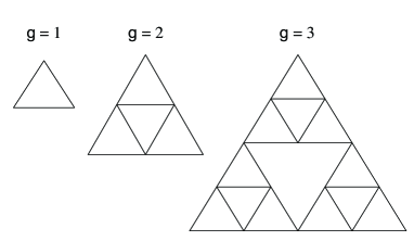
Figure 1: Construction of Sierpinski networks. A Sierpinski network of generation $g$ is denoted $\Delta_{g}$. The three networks shown in this figure are thus $\Delta_{1}$, $\Delta_{2}$ and $\Delta_{3}$.

It is well-known that Sierpinski networks are self-similar. For a Sierpinski network of generation $g$, the number of nodes is

$$n_{g}=\frac{3^{g}+3}{2}~{},$$ (2)

which is obtained of the recursion relation $n_{g+1}=3n_{g}-3$ with $n_{g=1}=3$. The number of edges is simply

$$m_{g}=3^{g}~{}.$$ (3)

For instance, a Sierpinski network of generation $g=6$ has $n_{g}=366$ nodes and $m_{g}=729$ edges.

2.2 Box-counting method by covering nodes

We first adapt the node-covering method used by Song, Havlin, and Makse [9] to cover the nodes of a Sierpinski network $\Delta_{g}$. Let us start with a box of size $\ell_{B}=\ell=1$. Actually, three geometrical patterns should be considered which are of box size $\ell=1$: (i) the triangle initiator $\Delta_{1}$, (ii) an edge of unit length with two nodes, and (iii) an individual node. We use these three geometrical patterns to cover the nodes of Sierpinski networks. Figure 2 shows the obtained coverings of $\Delta_{g}$ for $g=2$, $3$, $4$ and $5$ with boxes of size $\ell=1$. For instance, the optimal node-covering configuration of $\Delta_{2}$ is obtained with just one triangle initiator $\Delta_{1}$, one edge and one individual node. The optimal node-covering configuration of $\Delta_{3}$ uses three triangle initiators $\Delta_{1}$, three edges and zero individual nodes. And so on.

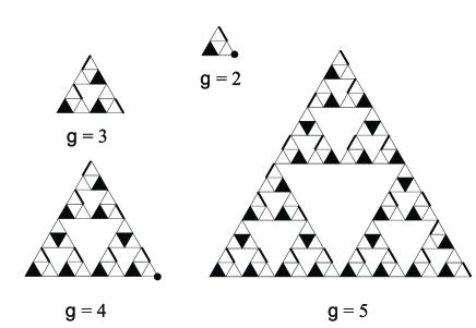
Figure 2: Iterative algorithm for tiling Sierpinski networks $\Delta_{g}$ for $g=2$, $3$, $4$ and $5$ with boxes of size $\ell=1$. The “boxes” are the triangle initiator $\Delta_{1}$, an edge of unit length with its two nodes (represented by as thick segments in the figure) and an individual node (represented as a small filled circle in the figure).

For a given network, its node-covering structure includes $N_{3}$ triangle initiators $\Delta_{1}$, $N_{2}$ edges, and $N_{1}$ nodes, giving a total number of covering boxes equal to $N_{V}=N_{1}+N_{2}+N_{3}$. Note that the number of nodes is given by $n_{g}=3N_{3}+2N_{2}+N_{1}$ because the optimal node-covering patterns involve no overlaps. For $g=1$, we have obviously $N_{V}(1)=1$. For $g\geq 2$, each Sierpinski network $\Delta_{g}$ can be viewed as made of $\Delta_{2}$ elements. For each $\Delta_{2}$ in a given $\Delta_{g}$, there is only one covering box which is a $\Delta_{1}$. For two adjacent $\Delta_{2}$’s, there are no additional $\Delta_{1}$ boxes. Therefore, the maximal number of boxes $\Delta_{1}$ used in the covering is

$$N_{3}^{\prime}=3^{g-2}~{}.$$ (4)

These $N_{3}^{\prime}$ $\Delta_{1}$ boxes cover $3N_{3}^{\prime}=3^{g-1}$ nodes. Therefore, the minimal number of nodes which are not covered by $\Delta_{1}$ boxes is $n_{g}-3N_{3}^{\prime}=\frac{3^{g}+3}{2}-3^{g-1}=\frac{3^{g-1}+3}{2}$. For this minimum number of still uncovered nodes, the maximum number of covering boxes that are edges (which we can refer to as “Min-Max”) is

$$N_{2}^{\prime}=\left[\frac{n_{g}-N_{3}^{\prime}}{2}\right]=\left[\frac{3^{g-1}+3}{4}\right]=\frac{3^{g-1}-(-1)^{g-1}}{4}+\frac{1+(-1)^{g-1}}{2}~{},$$ (5)

where $[x]$ is the integer part of $x$. Then, the remaining number of isolated nodes to cover with individual node boxes is

$$N_{1}^{\prime}=n_{g}-3N_{3}^{\prime}-2N_{2}^{\prime}=[1-(-1)^{g-1}]/2~{},$$ (6)

It follows immediately that

$$N_{V}\geq N_{1}^{\prime}+N_{2}^{\prime}+N_{3}^{\prime}=\frac{7\times 3^{g-2}+4+(-1)^{g}}{4}~{}.$$ (7)

In other words, because the total number of covering boxes is minimized by using the maximum number of $\Delta_{1}$’s (since each cover three nodes), the above construction shows that $N_{1}^{\prime}+N_{2}^{\prime}+N_{3}^{\prime}$ is the infimum of the minimal number $N_{V}$ of covering boxes.

For $g=2,3,4,5$, Fig. 2 provides one possible tiling for each, where the infimum $N_{1}^{\prime}+N_{2}^{\prime}+N_{3}^{\prime}$ is reached, i.e., the number of boxes is exactly $[{7\times 3^{g-2}+4+(-1)^{g}}]/{4}$. Together with Eq. (7), we synthesize the above results under the single expression

$$N_{V}=H(g-1.5)\times\frac{7\times 3^{g-2}+4+(-1)^{g}}{4}+H(1.5-g)~{},$$ (8)

where $H(x)$ is the Heaviside function. Our numerical calculations show that this equation holds for all $g>5$ cases that we have investigated. For the covering of a Sierpinski network $\Delta_{g}$ with boxes of size $\ell>1$, we do not have analytic expressions for $N_{V}(\ell)$. However, our numerical simulations show that $N_{V}(2^{k})=N_{E}(2^{k})$ for $1<k<g$, where the definition of $N_{E}$ is given in the next sub-section.

2.3 Box-counting method by covering edges

Instead of covering nodes as described in the previous sub-section, we propose to use boxes in order to cover all the edges. Mathematically, this problem can be described as follows. Consider the set $E$ of all the edges of a given network. Let $\{E_{i}:i=1,2,\cdots,N_{E}(\ell)\}$ be a partition of $E$, that is, $E_{i}\subseteq E$, $E_{i}\cap E_{j}=\Phi$ (null set) for $i\neq j$, and $E=\cup_{i=1}^{N_{E}(\ell)}E_{i}$. The size (or diameter) of $E_{i}$, denoted by $d(E_{i})$, is defined as the maximum distance among all possible pairs of nodes of $E_{i}$ counted as the number of edges to go from one node to the other of the pair. For a given $\ell$, we construct an edge-covering by partitioning the set $E$ into subsets $\{E_{i}\}$ such that all their diameters $d(E_{i})$ are smaller than or equal to $\ell$ for all $i$’s. Then, the partition $\{E_{i}:i=1,2,\cdots,N_{E}(\ell)\}$ is said to be a covering of the network with boxes of size $\ell$. We look for the best edge-covering structures by minimizing $N_{E}(\ell)$, for each $\ell$. An illustration of the edge-covering method is shown in Fig. 3 for three different values of $\ell$.

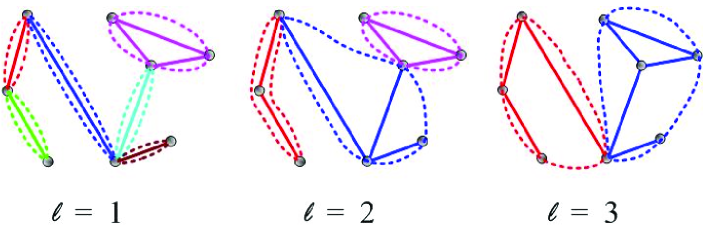
Figure 3: (Color online) Illustration of the edge-covering method for three different “box” sizes $\ell=1$, $2$, and $3$. The nodes of the network are the circles and the edges of the network are shown as solid lines. The closed dashed lines delineate the sub-sets or boxes of diameter no larger than $\ell$. For $\ell=1$, two subset topologies are possible: edges joining two adjacent nodes and a triplet of nodes forming a triangle which also has diameter $1$. For larger $\ell$, arbitrary complicated topologies for the sub-set/boxes are possible as long as their diameter remains smaller than or equal to $\ell$, as shown in the case $\ell=2$ and $\ell=3$. The edge-covering shown in the figure was obtained by our simulated annealing algorithm which provides in these simple cases optimal solutions.

Note that our algorithm for covering edges also automatically covers the nodes (sometimes with some nodes multiply covered). Thus, the minimal number $N_{E}(\ell)$ of boxes of a given size $\ell$ in the edge-covering method is not smaller than $N_{V}(\ell)$. Consider a $g$-generation Sierpinski network and scales $\ell=2^{k}$ with $k=0,1,2,\cdots,g-1$. It is well-known that

$$N_{E}(2^{k})=3^{g-1-k}~{}.$$ (9)

Therefore, we have

$$N_{E}(\ell)=3^{g-1}\cdot\ell^{-D_{E}}~{},$$ (10)

where $D_{E}=\ln(3)/\ln(2)\approx 1.5850$ is the fractal dimension. On the other hand, the scale invariance symmetry of the Sierpinski network can be expressed as

$$N_{E}(\ell)=3N_{E}(2\ell)~{}.$$ (11)

The general solution of this functional equation (11) takes the log-periodic structure

$$N_{E}(\ell)\sim\ell^{-D_{E}}\phi\left(\log_{2}(\ell)\right)~{},$$ (12)

where $\phi(x+1)=\phi(x)$ is a periodic function with unit period. Here, the preferred scaling ratio of the construction of the Sierpinski gasket is $\lambda=e^{\ln(2)}=2$, corresponding to a log-frequency $f=1$ (more generally when the scaling ratio is not $2$, we have $\phi(x+1/f)=\phi(x)$ and $\lambda=e^{\ln(2)/f}$).

2.4 Simulated annealing for the node-covering and edge-covering methods

According to the definition of fractal dimensions, we need to determine the minimal number of boxes necessary to cover the nodes or the edges of a network, as a function of the box scale $\ell$. In the supplementary materials of ref. [9], it was reported that “the minimization (of the number of boxes used to cover the network) is not relevant and any covering gives the same exponent”. While this may be true in some cases, working with arbitrary covering structures adds noise to the scaling laws. In order to get cleaner scaling, we have implemented the simulated annealing algorithm [21, 22] to obtain covering partitions with a minimum number of covering boxes.

The simulated annealing algorithm is implemented as follows. For the edge-covering problem, the network is viewed as a set of edges, which can be partitioned into “boxes” or subsets of connected edges. Starting from a given partition with $C$ boxes of sizes no larger than $\ell$, we consider three possible moves to transform the partition into a new one:

1. One edge is moved from one box with at least two edges in it to another box if the diameters of both new boxes do not exceed $\ell$;

2. One edge is moved out of one box with at least two edges to form a new box consisting of one edge; and

3. Two boxes merge to form a new box, a move which is allowed if the diameter of the resulting box is no larger than $\ell$.

At each temperature $T$, we perform $k_{1}$ edge operations of the first-type of edge exchanges between pairs of boxes, $k_{2}$ operations of the second-type to form new boxes, and $k_{3}$ operations of the third-type merging pairs of boxes. An operation is accepted with probability

$$p=\left\{\begin{array}[]{lll}1&{}{}&{\rm{if}}~{}~{}C_{a}\leqslant C_{b}\\ \exp\left(-\frac{C_{a}-C_{b}}{T}\right)&{}{}&{\rm{if}}~{}~{}C_{a}>C_{b}\end{array}\right.$$ (13)

where $C_{b}$ and $C_{a}$ are the numbers of boxes before and after an operation. After having performed $k_{1}+k_{2}+k_{3}$ possible operations, the system is cooled down to a lower temperature $T^{\prime}=cT$, where $c$ is a constant less than and close to $1$ (typically $c=0.995\sim 0.999$).

For the node-covering method, the simulated annealing procedure is deduced from the one described above by applying the three types of operations to nodes rather than to edges. Typical values for $k_{1},k_{2}$ and $k_{3}$ are 20000, 5, and 15. The much larger value of $k_{1}$ is justified by the fact that the single edge transfers should be much more frequent than merging two boxes and splitting one boxes into two. If $k_{2}$ and $k_{3}$ were much larger relative to $k_{1}$, it would be more difficult for the optimization to converge to a minimal box number. This is confirmed by our simulations.

2.5 Numerical comparison of the nodes-covering and edges-covering box-counting methods

We first compare the node-covering method developed in Ref. [9] and our edge-covering method by applying them on a Sierpinski network $\Delta_{6}$ of sixth generation. We have used the simulated annealing algorithm described above to search for the minimal numbers $N_{V}(\ell)$ and $N_{E}(\ell)$ of covering boxes of size $\ell$ for the two methods. The results are shown in Fig. 4. One can observe that $N_{V}(1)=143$ predicted by (8) and $N_{E}(2^{k})$ predicted by Eq. (9) are recovered by the simulations. Our simulations also confirm that $N_{V}(\ell)\leqslant N_{E}(\ell)$, as expected from the nature of the two methods.

Although the values of $N_{V}$ and $N_{E}$ are quite close, their difference is such that their corresponding estimations of the fractal dimension are significantly different. The apparent fractal dimension $D_{V}$ obtained using the node-covering method with equidistant integer values of $\ell$ gives $D_{V}=1.30$, which is the absolute slope of the line of $\ln N_{V}(\ell)$ versus $\ln\ell$ for $\ell=1,2,3,\cdots,32$ (see the dotted-dashed line in Fig. 4). The regression of $\ln N_{E}(\ell)$ (obtained with equidistant integer values of $\ell$) as a function of $\ln\ell$ for $\ell=1,2,3,\cdots,32$, shown as the dashed line, gives $D_{E}=1.37$. Both values are significantly biased downward compared with the exact analytical value $D_{f}=1.5850$. However, $D_{E}=1.37$ is a better estimate of $D_{f}$. These biases stem from the discrete-scale invariant structure of the Sierpinski network, which leads to geometrically increasing plateaus, as can be seen in Fig. 4. The estimated dimension $D_{E}$, while also biased, is closer to the exact value, because the Sierpinski network is exactly self-similar in terms of edges but only asymptotically self-similar in terms of nodes. This suggests that the edge-covering method may give better results for finite-sized networks.

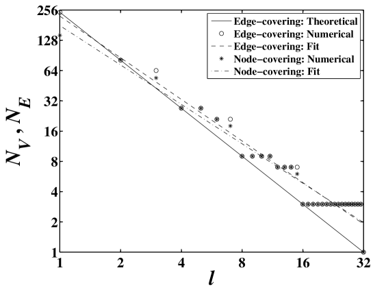
Figure 4: Comparison of simulations and theoretical analysis for the node-covering and edge-covering methods described in previous sections. The slope of the dotted-dashed (respectively dashed) line gives the estimation $D_{V}=1.30$ (respectively $D_{E}=1.37$) from the node-covering (respectively edge-covering) method. The exact analytical value is $D_{f}=1.5850$.

2.6 Log-periodic oscillations and referred scaling ratio

The data in Fig. 4 not only exhibits clear scaling behavior. In addition, there are log-periodic oscillations decorating the leading power law behavior, as expected from the theoretical considerations presented in Section 2.3. We now show how this log-periodicity can be extracted empirically from the data. To extract the log-frequency $f$ and the preferred scaling ratio $\lambda$, we first detrend $N_{E}$ by removing the power law to investigate the quantity

$$\ln\phi(\ln(\ell))=\ln N_{E}(\ell)-D_{E}\ln\ell~{},$$ (14)

where $D_{E}$ is estimated as the negative of the slope of the linear regression of $\ln(N_{E})$ as a function of $\ln(\ell)$. It is convenient to consider the right-side continuous function $N_{E}(\ell)$ for $1\leqslant\ell\leqslant 32$ defined as

$$N_{E}(\ell)=N_{E}(i),~{}{\mathrm{if}}~{}~{}i\leqslant\ell<i+1~{},$$ (15)

where $i=1,2,\cdots,32$. The dependence of $N_{E}(\ell)$ as a function of $\ell$ is shown in Fig. 5a. The dependence of $\ln_{2}\phi$ obtained from (14) as a function of $\ln_{2}\ell$ is shown in Fig. 5b.

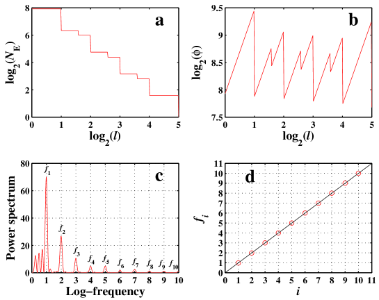
Figure 5: Quantification of log-periodicity in the Sierpinski network. a: dependence of $N_{E}(\ell)$ defined by (15) as a function of $\ell$. b: dependence of $\phi$ as a function of $\ell$ in log-log scale, showing strong visual evidence of the log-periodic oscillations. c: Power spectrum of the function $\log_{2}[\phi(\log_{2}\ell)]$ of the variable $\log_{2}\ell$. The log-frequency of the main peak is $f_{1}=0.985$ corresponding to the preferred scaling ratio is $\lambda=2.02$. d: dependence of the log-frequencies $f_{i}$ corresponding to the successive peaks shown in panel c as a function of their index $i$. The linear dependence suggests that the succession of peaks in panel c corresponds to the different harmonics of $f_{1}$. A new estimation of $f_{1}$ is obtained by the regression $f_{i}=i\times f_{1}$, which yields $f_{1}=1.002$ corresponding to a preferred scaling ratio $\lambda=1.997$.

In order to calculate the power spectrum of the function $\log_{2}[\phi(\log_{2}(\ell))]$ of the variable $\log_{2}\ell$, we sample on 300 values with regularly spacing in $[\log_{2}(1),\log_{2}(32)]$. The resulting power spectrum is shown in Fig. 5c. The log-frequency (in logarithm with base $2$) associated with the highest peak is $f_{1}=0.985$ and the preferred scaling ratio is therefore $\lambda=e^{(\ln 2)/f}=2^{1/f}=2.021$. The height of the highest peak is $69.9$, which together with the number of data points gives a probability of false-positive for log-periodicity essentially $0$, at all confidence levels [23]. In addition to the main peak in panel c of Fig. 5, many secondary peaks can be observed. They are found to be equidistant to a very good approximation, suggesting that the corresponding log-frequencies are nothing but the harmonics $f_{2}=2f_{1},f_{3}=3f_{1},\cdots,f_{i}=i\times f_{1},\cdots$ of the fundamental log-frequency $f_{1}$. The existence of a set of harmonics is known to increase the evidence of log-periodicity [24]. In addition, the measurements of the harmonic log-frequencies allows us to improve the estimation of the fundamental log-frequency $f_{1}$ by using a linear regression of $f_{i}$ as a function of $i$ [24], as shown in Fig. 5d. The slope of this regression gives $f=1.002$ and the corresponding preferred scaling ratio is $\lambda=1.997$, which are very close to the exact values $f_{1}=1$ and $\lambda=2$ respectively for the Sierpinski network.

2.7 How to use log-periodicity to improve the estimation of the fractal dimension

Note that a regression of $\ln N_{E}(\ell)$ versus $\ln\ell$ for equidistant integer values of $\ell=1,2,3,4,5,\cdots,32$ gives a biased estimate of the fractal dimension $D_{E}=1.37$, which is significantly smaller than the exact value $D_{f}=1.5850$. In contrast, sampling $\ell$ with a uniform logarithmic spacing as in Sec. 2.6 (with 300 points) gives $D_{E}=1.52$, much closer to the exact value.

More specifically, we stress the general property that a fractal system with discrete scale invariance is better sampled using data points at $\ell=\ell_{0}\lambda^{k}$, where $\ell_{0}$ is associated with a well-chosen phase of the log-periodicity and $k=0,1,2,3\cdots$, which are integer powers of the underlying discrete scale factor $\lambda$. In this way, the sub-dominant log-periodic corrections to the scaling are removed.

Using this method for sampling $N_{E}(\ell)$, i.e., regressing $\ln N_{E}(1)$, $\ln N_{E}(2)$, $\ln N_{E}(4)$, $\ln N_{E}(8)$, $\ln N_{E}(16)$, and $\ln N_{E}(32)$ for the Sierpinski network $\Delta_{6}$ as a function of $\ell=1$, 2, 4, 8, 16, and 32, gives $D_{E}=1.5850$ which is indeed the exact fractal dimension $D_{f}$.

Thus, we decrease the bias in the estimate of the scaling exponent $D_{E}$ when going from equidistant integer values of $\ell$ to geometrically sampled $\ell$. Moreover, we eliminate completely the bias when the geometrical ratio used in the sampling method is equal to the preferred scaling ratio $\lambda$ characterizing the discrete scale invariant structure of the network.

Obviously, this method applies and work for other fractals only if they exhibit the symmetry of discrete scale invariance. In our experience, using $\ell_{0}=1$ is a good choice.

3 Application to cellular networks

3.1 The data sets

We use the ERGO (formerly WIT) database, which provides links to information about the functional role of enzymes. More precisely, the ERGO database of cellular networks considers the cellular functions divided according to bioengineering principles containing data sets for intermediate metabolism and bioenergetics (core metabolism), information pathways, electron transport, and transmembrane transport. We revisit the forty three cellular networks, which have been studied in a recent analysis developed from the point of view of scale-free networks [25].

3.2 Log-periodic oscillations in cellular networks

We consider the same 43 cellular networks analyzed in [25]. We follow the procedure described in Sec. 2 to investigate each of these 43 cellular networks. Specifically, we implement the edge-covering method with the simulated annealing algorithm to find the minimal number $N_{E}(\ell)$ of boxes of size $\ell$ that cover all the edges of a given network. We find that there is a power law dependence of $N_{E}(\ell)$ upon $\ell$ with exponent $-D_{E}$. In order to extract the best minimally biased estimate of $D_{E}$, following the recommendations of the previous section, we first prune $N_{E}(\ell)$ by using Eq. (15). We then perform a logarithmically evenly spaced sampling on 300 values. Then, we detrend $N_{E}(\ell)$ by the power law $\ell^{-D_{E}}$ to obtain $\phi(\ell)$, as shown in Fig. 6b. Fourier transform is adopted to obtain the power spectrum of $\log_{2}(\phi)$ with $\log_{2}(\ell)$ being the independent variable, as shown in Fig. 6c. A clear peak at about $f=1$ as well as many remarkable harmonic peaks at $f_{i}=if$ are observed for all the cellular networks. For several networks, the peak at $f\approx 1$ is not the highest peak. However, the harmonic peaks give strong evidence that $f\approx 1$ is the fundamental log-frequency. In addition, the high peaks at $f\approx 0.25$ are nothing but a Nyquist frequency (in log-scale) corresponding to the lower frequency approximately equal to half the inverse of the whole interval (in log-scale). The total span of the data is about $\log_{2}18$ and its low-frequency is $1/\log_{2}18\approx 0.24$, known as the most probable log-frequency [26]. The averaged log-frequency over all networks is thus $f=0.97\pm 0.05$ and the average preferred scaling ratio if $\lambda={\rm{e}}^{\log(2)/f}=2.05\pm 0.07$. We also plot $f_{i}$ versus $i$ to achieve a better estimate of the fundamental log-frequency, as shown in Fig. 6d. We see that all plots show excellent linearity. This gives an averaged log-frequency over all networks is thus $f=0.996\pm 0.004$ and the average preferred scaling ratio if $\lambda={\rm{e}}^{\log(2)/f}=2.005\pm 0.005$.

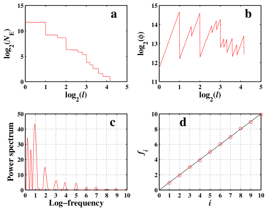
Figure 6: Log-periodicity in the Aquifex aeolicus network. a, The dependence of $N_{E}(\ell)$ as a function of $\ell$. b, The dependence of $\phi$ as a function of $\ell$. The log-periodic oscillations are very clear. c, Power spectrum of $\log_{2}[\phi(\log_{2}(\ell))]$. The log-frequency is $f_{1}=0.9413$ and the preferred scaling ratio is $\lambda=2.0884$. The probability of false alarm is 7.2%. d, The dependence of $f_{i}$ as a function of $i$. The log-frequency is $f=0.9990$ and the preferred scaling ratio is $\lambda=2.0014$.

We now present two additional methods to obtain the averaged log-frequency.

The first method consists in a canonical analysis of the log-periodic oscillations in which we perform averaging over all individual power spectra to get an averaged spectrum. The idea was initially introduced in the analysis of log-periodicity in two-dimensional turbulence [27]. Figure 7 shows the averaged power spectrum over 43 cellular networks. The highest peak is located at $f_{1}=0.965$ (thus $\lambda=2.051$). Again we see a number of harmonic peaks at $f_{i}=if$. Linear regression of $f_{i}$ against $i$, shown in the inset of Fig. 7, gives a nice line with slope $f=1.0001$ (thus $\lambda=1.9998$), which is the fundamental log-frequency.

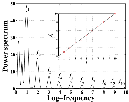
Figure 7: Power spectrum obtained by canonical averaging over all power spectra for 43 cellular networks. Inset: Estimation of the fundamental log-frequency.

The second method is to average $N_{E}(\ell)$ for each $\ell$ over the 43 networks, which is then analyzed as if it is from an individual network. The highest peak is located at $f_{1}=0.989$ (thus $\lambda=2.015$). Again we observe a number of harmonic peaks at $f_{i}=if$. Linear regression of $f_{i}$ against $i$, shown in the inset of Fig. 7, gives a nice line with slope $f=0.999$ (thus $\lambda=2.002$), which is the fundamental log-frequency.

3.3 The significance of log-periodicity

There are well established methods to assess the statistical significance of log-periodic oscillations according to the data points used in the analysis and the Lomb peak height [23].

Here, in order to test for the possibility that the log-periodic oscillations could be artifactual, we adopt the following bootstrapping approach. For each cellular network, we obtain the minimal number of boxes needed to cover all the edges of the network using simulated annealing. Due to the self-similarity of the network, we can calculate the residuals $\phi$ according to Eq. (14). Then we reshuffle the residuals series randomly to get a new reshuffled residuals series $\phi^{\prime}$ and then put it back to construct a new series of edge-covering box numbers $N^{\prime}_{E}=\phi^{\prime}\ell^{-D_{E}}$. Then we use the same procedure described in Sec. 3.2 to construct the power spectrum. We extract the maximum height $P_{m}$ of the part with log-frequency between $[0.9,1.1]$. This procedure is repeated for 1000 times, which gives 1000 values of $P_{m}$. For the real cellular network, we have its counterpart height $P_{N}$. Finally, the probability of a false alarm for log-periodicity (so-called “false positive” or error of type II) is defined by

$$\Pr=\frac{\#[P_{m}>P_{N}]}{1000}~{},$$ (16)

where $\#[P_{m}>P_{N}]$ counts the number of networks whose Lomb peak height is larger than $P_{N}$.

The resulting probabilities of a false alarm for each of the 43 cellular networks are ordered by increasing values: 0.0040; 0.0060; 0.0080; 0.0090; 0.0120; 0.0140; 0.0160; 0.0160; 0.0170; 0.0170; 0.0180; 0.0210; 0.0220; 0.0220; 0.0270; 0.0300; 0.0330; 0.0390; 0.0430; 0.0510; 0.0510; 0.0580; 0.0620; 0.0700; 0.0710; 0.0720; 0.0730; 0.0770; 0.0790; 0.0830; 0.0840; 0.0880; 0.0910; 0.1010; 0.1110; 0.1120; 0.1230; 0.1500; 0.1630; 0.1640; 0.1660; 0.2250; 0.2360. We find that 19 out of the 43 cellular networks have significant log-periodicity above the confidence level of 95% ($\Pr<0.05$) and 33 out of the 43 cellular networks have significant log-periodicity at the confidence level of 90% ($\Pr<0.10$). However, there are 10 cases that the null hypothesis that the log-periodicity is an artifact can not be rejected even at the significance level of 10%.

3.4 A simple artifactual contribution to the observed log-periodicity

The reported probabilities of a false positive for log-periodicity are not very small, which cast doubts on whether log-periodicity really exists. Another curious fact is the closeness of the measured scaling factor $\lambda$ to the number $2$. This last fact suggests an artifact. Actually, there is a simple mechanism to produce peaks at $\lambda\approx 2$ in finite networks (the effect disappears eventually in the log-periodic spectral analysis for infinitely large networks). The mechanism is based on the fact that the edges are discrete and $\ell$ is an integer. Since $\ell$ takes integer values, the two smallest values $\ell=1$ and $\ell=2$ allow to form the ratio $2$. Then, the next two values $\ell=3$ and $4$ gives the ratios $3/2$ and $4/2=2$. Combined with the two first values $\ell=1,2$, the “harmonic” $4/1$ appear. We thus see that two approximate log-periodic oscillations appear when $N_{E}(\ell)$ is sampled at intermediate real values (we use typically 300 values of geometrically spaced $\ell$’s over a range of scale roughly $18$), just from the existence of discreteness in the first four values of $\ell$. This effect can be approximately observed in Fig. 6b: the two first oscillations are well-formed up to $\log_{2}(\ell)=2$, i.e., for $\ell$ up to the value $4$ as just described. In other words, any power law function which is sampled on integers will exhibit some observable log-periodicity with two to three approximate oscillations, just as a result of discretization for the first few integer values of the scale. This idea is confirmed by our synthetic bootstrap tests which, in complete absence of log-periodicity (which is destroyed by the random reshuffling), nevertheless produce peaks $P_{m}$ in the log-periodic spectral analysis which are often comparable to those observed in the 43 networks, hence the relatively large values of $\Pr$ (defined in Eq. (16)) obtained in the previous section.

We conclude this rather pessimistic argument (with respect to the existence of genuine log-periodicity) by two positive notes.

• First, notwithstanding this artificial effect, one cannot deny that the real cellular networks have often higher Lomb peaks for log-periodicity than the reshuffled ones, suggesting other sources of discrete scale invariance, perhaps genuine. If this is the case, the value $\lambda\approx 2$ remains to be explained. The simplest argument could be that the dichotomous discrete hierarchy is perhaps the most natural and most robust discrete hierarchy that can be found.

• Second, as we have shown in section 2, taking into account the presence of log-periodicity, spurious or not, to sample $N_{E}(\ell)$ offers a priori a better less-biased estimator for the fractal dimension $D_{E}$.

3.5 Fractal dimensions of cellular networks

We revisit in this section the estimation of fractal dimensions of the 43 cellular networks using four different methods described below. Note that all these methods are based on the edge-covering method.

• Method 1. We have shown in Sec. 3.2 that there are significant log-periodic oscillations in all the 43 cellular networks with a universal preferred scaling ratio $\lambda=2$. We can the use the data points at $\ell=2^{k}$: $N_{E}(1)$, $N_{E}(2)$, $N_{E}(4)$, $\cdots$, shown in Fig. 8 as stars. The inverse slope of $\ln[N_{E}(2^{k})]$ against $\ln(\ell_{k})=k\ln 2$ is an estimate of the fractal dimension. This method is illustrated in Fig. 8.

• Method 2. This method uses a logarithmic sampling using Eq. (15). For each network, 300 evenly spaced data points in the logarithmic abscissa are used and its inverse slope of the data in log-log plot is an estimate of the fractal dimension.

• Method 3. This method uses all the data point at $\ell=1,2,3,\cdots$, shown as circles in Fig. 8, and fit it in log-log plot. The inverse of the slope is taken as the estimate of the fractal dimension. This method is also illustrated in Fig. 8.

• Method 4. This method is the same as Method 3 except that this method plot $\ln[N_{E}(\ell)]$ versus $\ln(\ell+1)$, as used in [9].

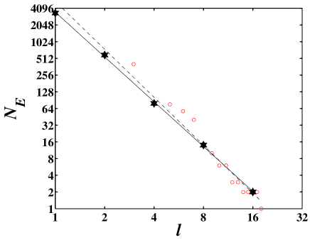
Figure 8: Determination of the fractal dimensions. The solid line is a fit to the data points at $\ell=2^{k}$ using Method 1. The dashed line is the fit to all data points with Method 3. The open circles are all the calculated values of $N_{E}$ for all integer $\ell$’s while the stars are sampled geometrically at $\ell_{k}=2^{k}$.

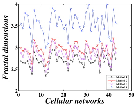
Figure 9: Comparison of the fractal dimensions of the 43 cellular networks estimated using four different methods.

We calculated the fractal dimensions of the 43 cellular networks using these four different methods. The results are shown in Fig. 9. The averages of the estimated fractal dimensions are $D_{E}=2.68\pm 0.15$ (method 1), $D_{E}=2.95\pm 0.15$ (method 2), $D_{E}=2.84\pm 0.19$ (method 3), and $D_{E}=3.47\pm 0.27$ (method 4), respectively. It is interesting to note that $D_{E}=3.54\pm 0.27$ for Method 4 is identical to $D_{V}=3.5$ estimated using node-covering [9]. We argue that our Method 1 based on the log-periodic sampling gives a better and more robust estimation of the fractal dimension, due to a minimal bias. We believe that our method of edge-covering with simulated annealing and log-periodic sampling minimizes the significant bias in the log-log regression.

4 Conclusion

In summary, we have proposed a new box-counting method for networks, in which boxes are tiled to cover all the edges of the network. The minimal number $N_{E}$ of boxes of size $\ell$ in the edge-covering method is obtained by a simulated annealing algorithm. We have performed detailed analytical and numerical analysis of the Sierpinski network. The results show that the Sierpinski network is strictly self-similar only when using the edges (and not the nodes). We have shown that the node-covering method gives a stronger downward bias estimate of the fractal dimension of the Sierpinski network.

In addition, we have shown that we can use the discrete scale invariance of the Sierpinski network to characterize the log-periodic oscillations in $N_{E}(\ell)$ and develop a method which removes completely the bias in the estimation of the fractal dimension $D_{E}$. Taking into account the presence of log-periodicity to adapt the sampling of the function $N_{E}(\ell)$ allows us to design a better estimator for the fractal dimension of self-similar networks.

We have applied this improved method to 43 cellular networks previously studied in the literature. We found that $N_{E}$ scales with respect to $\ell$ as a power law $N_{E}\sim\ell^{-D_{E}}$ with the fractal dimension $D_{E}=2.67\pm 0.15$. Some of the cellular networks exhibit log-periodic oscillations in $N_{E}$. However, a bootstrapping statistical test shows that the existence of log-periodicity in cellular networks is not fully conclusive.

Acknowledgments: This work was supported by the National Natural Science Foundation of China (Grant No. 70501011) and the Fok Ying Tong Education Foundation (Grant No. 101086).

References

- [1] R. Albert, A.-L. Barabási, Statistical mechanics of complex networks, Rev. Mod. Phys. 74 (2002) 47–97.
- [2] M. E. J. Newman, The structure and function of complex networks, SIAM Rev. 45 (2) (2003) 167–256.
- [3] S. N. Dorogovtsev, J. F. F. Mendes, Evolution of Networks: From Biological Nets to the Internet and the WWW, Oxford University Press, Oxford, 2003.
- [4] D. J. Watts, S. H. Strogatz, Collective dynamics in ‘small-world’ networks, Nature 393 (1998) 440–442.
- [5] A.-L. Barabási, R. Albert, Emergence of scaling in random networks, Science 286 (1999) 509–512.
- [6] E. F. Keller, Revisiting “scale-free” networks, BioEssays 27 (2005) 1060–1068.
- [7] D. Sornette, Critical Phenomena in Natural Sciences - Chaos, Fractals, Self-organization and Disorder: Concepts and Tools, 2nd Edition, Springer, Berlin, 2004.
- [8] M. E. J. Newman, Detecting community structure in networks, Eur. Phys. J. B 38 (2004) 321–330.
- [9] C.-M. Song, S. Havlin, H. A. Makse, Self-similarity of complex networks, Nature 433 (2005) 392–395.
- [10] B. Mandelbrot, The Fractal Geometry of Nature, W. H. Freeman, New York, 1983.
- [11] B. J. Kim, Geographical coarse graining of complex networks, Phys. Rev. Lett. 93 (2004) 168701.
- [12] J. Feder, Fractals, Plenum Press, New York, 1988.
- [13] S. H. Strogatz, Romanesque networks, Nature 433 (2005) 365–366.
- [14] S.-H. Yook, F. Radicchi, H. Meyer-Ortmanns, Self-similar scale-free networks and disassortativity, Phys. Rev. E 72 (2005) 045105.
- [15] C.-M. Song, S. Havlin, H. A. Makse, Origins of fractality in the growth of complex networks, Nat. Phys. 2 (2006) 275–281.
- [16] K.-I. Goh, G. Salvi, B. Kahng, D. Kim, Skeleton and fractal scaling in complex networks, Phys. Rev. Lett. 96 (2006) 018701.
- [17] J. S. Kim, K.-I. Goh, G. Salvi, E. Oh, B. Kahng, D. Kim, Fractality in complex networks: Critical and supercritical skeletons, cond-mat/0605324 (2006).
- [18] D. Sornette, Discrete scale invariance and complex dimensions, Phys. Rep. 297 (1998) 239–270.
- [19] K. Suchecki, J. A. Holyst, Log-periodic oscillations in degree distributions of hierarchical scale-free networks, Acta Physica Polonica B 36 (2005) 2499–2511.
- [20] M. Graña, J. P. Pinasco, Discrete scale invariance in scale free graphs, cond-mat/0602337 (2006).
- [21] S. Kirkpatrick, C. J. Gelatt, M. Vecchi, Optimization by simulated annealing, Science 220 (1983) 671–680.
- [22] A. Basu, L. N. Frazer, Rapid determination of the critical temperature in simulated annealing inversion, Science 249 (1990) 1409–1412.
- [23] W.-X. Zhou, D. Sornette, Statistical significance of periodicity and log-periodicity with heavy-tailed correlated noise, Int. J. Mod. Phys. C 13 (2002) 137–170.
- [24] W.-X. Zhou, D. Sornette, Evidence of intermittent cascades from discrete hierarchical dissipation in turbulence, Physica D 165 (2002) 94–125.
- [25] H. Jeong, B. Tombor, R. Albert, Z. N. Oltavi, A.-L. Barabási, The large-scale organization of metabolic networks, Nature 407 (2000) 651–654.
- [26] Y. Huang, A. Johansen, M. W. Lee, H. Saleur, D. Sornette, Artifactual log-periodicity in finite-size data: Relevance for earthquake aftershocks, J. Geophys. Res. 105 (2000) 25451–25471.
- [27] A. Johansen, D. Sornette, A. Hansen, Punctuated vortex coalescence and discrete scale invariance in two-dimensional turbulence, Physica D 138 (2000) 302–315.