Generating Spin Currents in Semiconductors with the Spin Hall Effect

Abstract

We investigate electrically-induced spin currents generated by the spin Hall effect in GaAs structures that distinguish edge effects from spin transport. Using Kerr rotation microscopy to image the spin polarization, we demonstrate that the observed spin accumulation is due to a transverse bulk electron spin current, which can drive spin polarization nearly 40 microns into a region in which there is minimal electric field. Using a model that incorporates the effects of spin drift, we determine the transverse spin drift velocity from the magnetic field dependence of the spin polarization.

The spin Hall effect refers to the generation of a spin current transverse to a charge current in non-magnetic systems in the absence of an applied magnetic field. This spin current may arise from spin-dependent scattering dyakonov ; hirsch or from the effect of the spin-orbit interaction on the band structure murakami ; sinova . Although spin current is difficult to measure directly, the spin Hall effect was predicted to create spin accumulation at the edges of a channel zhang . This electrically-induced spin polarization was observed in bulk epilayers of electron-doped semiconductors katoSHE and in two-dimensional hole wunderlich and electron systems sih , and recent calculations engel ; tse06 ; nomura show reasonable agreement with the experimental results. However, determining the spin current through analysis of the spin accumulation is complicated because spin is not a conserved quantity in the presence of the spin-orbit interaction rashba ; shi and the choice of boundary conditions has a strong effect on the calculated spin accumulation tse05 ; galitski . In addition, it is possible that spin polarization observed at the sample edges could be due to an edge effect, such as depletion near the edge resulting in a local spin splitting from the Bychkov-Rashba effect bychkov and not due to a bulk spin current. This local spin splitting could result in an electrically-induced spin polarization, similar to the spatially-homogenous polarization that has been measured in strained semiconductors katoCISP and semiconductor heterostructures sih ; silov .

In order to clarify the origin of the electrically-induced spin polarization, we design structures in which the effects of the boundary of the electric field are separated from edge effects. We fabricate mesas with transverse channels to allow spins to drift into regions in which there is minimal electric current. Using Kerr rotation microscopy, we observe the generation of a transverse bulk electron spin current created by a longitudinal voltage, which can cause spins to drift nearly 40 microns into a transverse channel. In addition, we determine the spin drift velocity from the magnetic field-dependence of the measured spin polarization.

The thin-film samples were fabricated from a 2 $\mu$m-thick epilayer of n-doped GaAs, with a Si doping density $n$ = 3 $\times$ 10¹⁶ cm^-3. The n-GaAs epilayer and the underlying 2 $\mu$m of undoped Al_0.4Ga_0.6As were grown on a (001) semi-insulating GaAs substrate using molecular beam epitaxy. Mesas were patterned using photolithography and a chemical etch, and ohmic contacts were made with annealed AuGe [Fig. 1(a)]. Each mesa consists of a main channel, fabricated along the [1$\overline{1}$0] direction along which the electric field is applied, and two smaller channels that extend from the main channel in the transverse direction. The main channels have length $l$ = 316 $\mu$m and width $w$ = 60 $\mu$m, and the transverse channels are 40 $\mu$m wide. One mesa has transverse channels that extend out 10 and 20 $\mu$m from the side of the channel, and the other mesa has side arms that are 30 and 40 $\mu$m long.

The samples are measured in a low-temperature scanning Kerr microscope stephens and mounted such that the main channels are perpendicular to the externally applied in-plane magnetic field. In order to measure the spin polarization, a linearly polarized beam is tuned to the absorption edge of the sample (wavelength $\lambda$ = 825 nm) and is incident upon the sample through an objective lens, which provides $\sim$1 $\mu$m lateral spatial resolution. The rotation of the polarization axis of the reflected beam is proportional to the electron spin polarization along the beam ($z$) direction. A square wave voltage with amplitude $V$/2 and frequency 1168 Hz is applied to the device for lock-in detection. We perform our measurements at a temperature T = 30 K, and we take the center of the channel to be the origin.

Kerr rotation is measured as a function of magnetic field (B) and position ($x$, $y$). In Figure 1(b), we show data for a position near the edge of the channel and away from either side arm ($x$ = 26 $\mu$m, $y$ = 0 $\mu$m). The data is the electrically-induced spin polarization and can be explained as spin polarization along the $z$ direction, which dephases and precesses about the applied magnetic field. This behavior is known as the Hanle effect opticalorientation , and the curve can be fit to a Lorentzian function A/[($\omega_{L}$ $\tau_{s}$)² + 1] to determine the amplitude A and transverse spin coherence time $\tau_{s}$. The Larmor precession frequency $\omega_{L}$ = g $\mu_{B}$ B/$\hbar$, where g is the electron g-factor (g = -0.44 for this sample as measured using time-resolved Kerr rotation crooker97 ), $\mu_{B}$ is the Bohr magneton, and $\hbar$ is Planck’s constant divided by 2$\pi$.

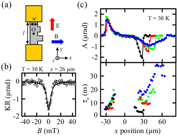
Figure 1: (color) (a) Measurement schematic and experimental geometry. We take the center of the channel to be the origin O. (b) Kerr rotation as a function of magnetic field at ($x$,$y$) = (26 $\mu$m, 0 $\mu$m). Line is a Lorentzian fit from which the amplitude and spin lifetime can be determined. (c) (top) Spin polarization amplitude as a function of position measured for the channel (black) and with 10 $\mu$m (red), 20 $\mu$m (green) and 40 $\mu$m (blue) side arms. (bottom) Spin coherence time as a function of position. Data are taken at T = 30 K.

We repeat this measurement for positions across the channel and the side arms. Figure 1(c) shows the amplitude and spin coherence times for the 60 $\mu$m wide channel and for the channel with 10 $\mu$m, 20 $\mu$m and 40 $\mu$m side arms. We observe that the spin polarization amplitude near the edge at $x$ = -30 $\mu$m is unchanged by the addition of the side arms. In contrast, the spin accumulation near $x$ = 30 $\mu$m is modified in the presence of the side arms, and the spin accumulation has a different spatial profile that is dependent on the side arm length. First, we notice that the spin accumulation is not always largest near the mesa edge. This is a clear indication that the spin polarization is not a local effect caused by the sample boundary. In addition, at any position $x$, the amplitude of the spin polarization is smaller for longer side arms. This is an indication that we are observing the spins drifting from the main channel and towards the end of the side arms.

The magnetic field dependence of the spin polarization is also different in the side arms. Using the Hanle model, the width of the field scans yields the spin coherence time. Near the edge at $x$ = -30 $\mu$m, we observe that the spin coherence time appears to increase for positions closer to the center of the channel, as reported in Ref. [katoSHE, ]. In the side arms, the spin coherence time appears to increase even more for positions farther from the edge of the channel. As noted in Ref. [katoSHE, ], this spatial dependence could be an effect on the lineshape due to the time that it takes for the spins to drift or an actual change in the spin coherence time for the spins that have diffused from the edge. Here we will show that the change in the lineshape in the transverse channels is not due to an actual change in spin lifetime but can be explained using a model that incorporates spin drift crooker05 ; lou .

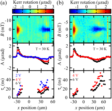
Figure 2: (color) (a) Measurements of the channel with a 20 $\mu$m side arm at T = 30 K. The edges of the main mesa are at $x$ = -30 $\mu$m and $x$ = +30 $\mu$m. Top panel is a color plot of Kerr rotation as a function of magnetic field and position for $V$ = 6 V. Middle panel shows the amplitude as a function of position for $V$ = 2 V (blue), 4 V (red) and 6 V (black). Bottom panel shows the spin coherence time as a function of position for $V$ = 2 V (blue), 4 V (red) and 6 V (black). (b) Measurements of the channel with a 40 $\mu$m side arm at T = 30 K. Top panel is a color plot of spin polarization as a function of magnetic field and position for $V$ = 6 V. Middle panel shows the amplitude as a function of position for $V$ = 4 V (red) and 6 V (black). Bottom panel shows the spin coherence time as a function of position for $V$ = 4 V (red) and 6 V (black). For the color plots, a vertical offset is subtracted from each magnetic field scan.

We examine the electric field dependence of the spin accumulation by performing spatial scans for different voltages. In Figure 2(a), we present measurements of the channel with a 20 $\mu$m side arm, and in Figure 2(b), we present measurements of the channel with a 40 $\mu$m side arm. The top panel shows the spin polarization as a function of applied magnetic field and position for $V$ = 6 V, and the amplitude and spin coherence time are shown below. From the color plots, the spatial dependence of the width of the field scans is apparent. We find that the amplitude of the measured polarization increases and the spin coherence time decreases with increasing voltage.

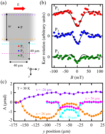
Figure 3: (color) (a) Measurement schematic showing sample dimensions. P indicates the position ($x$,$y$) = (0 $\mu$m, -50 $\mu$m). (b) Kerr rotation as a function of magnetic field for three different $x$ positions at $y$ = -50 $\mu$m on the 40 $\mu$m side arm. Taking $x$ = 0 $\mu$m to be the center of the channel, the edges of the main channel are at $x$ = -30 $\mu$m and x = +30 $\mu$m ($w$ = 60 $\mu$m). Measurements are shown for $x$ = 40 $\mu$m (P₁, red), $x$ = 50 $\mu$m (P₂, blue) and $x$ = 60 $\mu$m (P₃, green). Solid black lines are calculated from a model that accounts for spin drift, as described in the text. The same values for S₀, $\tau_{s}$, v_sd and $D$ are used for all three curves. (c) Amplitude of Kerr rotation measured as a function of longitudinal position $y$ for $x$ = -26 $\mu$m (purple), $x$ = 26 $\mu$m (orange), $x$ = 36 $\mu$m (cyan) and $x$ = 56 $\mu$m (magenta). These positions are shown as dashed lines in part (a) of this figure. One contact edge is located at $y$ = -158 $\mu$m, and the edges of the side arm are at $y$ = -70 $\mu$m and $y$ = -30 $\mu$m.

The Hanle model assumes a constant rate of spin generation, but this does not accurately reflect what occurs in the side arms, where there should be minimal electric current. Instead, we must consider a model that takes into account the fact that the spins are generated in the main channel and then drift into the side arm crooker05 ; lou . This signal is computed by averaging the spin orientations of the precessing electrons over the Gaussian distribution of their arrival times. For spins injected with an initial spin polarization S₀ along the $z$ direction at x₁ and then flow with a spin drift velocity v_sd before they are measured at a position x₂,

$$S_{z}(x_{1},x_{2},B)=\int_{0}^{\infty}\frac{S_{0}}{\sqrt{4\pi Dt}}e^{-(x_{2}-x_{1}-v_{\mathrm{sd}}t)^{2}/4Dt}e^{-t/\tau_{s}}$$

$$\times\cos(\omega_{L}t)dt$$ (1)

where $D$ is the spin diffusion constant. S_z($x_{2}$, B) is computed by integrating $x_{1}$ over the width of the main channel, from -30 $\mu$m to +30 $\mu$m. We apply this model to measurements taken on the 40 $\mu$m side arm, a schematic of which is shown in Fig. 3(a). Using resonant spin amplification kikkawa , we determine $\tau_{s}$ = 11.4 ns. The same set of parameters is used to calculate S_z($x$, B) for three positions in the side arm. As shown in Fig. 3(b), the model can reproduce the spatial dependence of the amplitude and lineshape using $D$ = 10 cm²/s and v_sd = 1.6 $\times$ 10⁵ cm/s and without assuming a spatially-dependent spin lifetime. The value obtained for v_sd may have a contribution from electric field gradients in the transverse channel, as well as the spin Hall effect.

To check the uniformity of the spin polarization along the longitudinal ($y$) direction, we perform spatial scans along the channel and across the side arms. We show the amplitude as determined from Lorentzian fits in Figure 3(c). The contact is located at $y$ = -158 $\mu$m, and from the scans taken at $x$ = -26 $\mu$m and $x$ = 26 $\mu$m, we see that the amplitude of the spin polarization builds up from zero at the contact to a maximum value over  50 $\mu$m. While the amplitude of the scans taken at $x$ = -26 $\mu$m are insensitive to the position of the side arm, which has edges at $y$ = -70 $\mu$m and $y$ = -30 $\mu$m, the measurements at $x$ = 26 $\mu$m show that the amplitude drops near the side arm due to spin drift into the side arm. Measurements taken across the side arm, at $x$ = 36 $\mu$m and $x$ = 56 $\mu$m, show that the amplitude is largest near the edges of the side arm, which may also be due to spin drift.

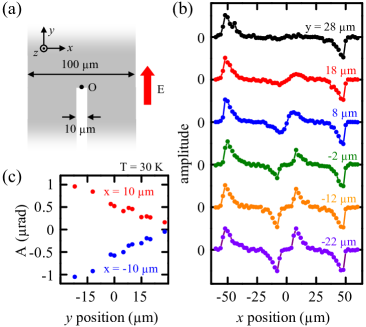
Figure 4: (color) (a) Measurement schematic showing a channel that splits into two smaller channels. O indicates the origin. (b) Kerr rotation amplitude as a function of transverse position $x$ for longitudinal positions $y$ = 28 $\mu$m (black), $y$ = 18 $\mu$m (red), $y$ = 8 $\mu$m (blue), $y$ = -2 $\mu$m (green), $y$ = -12 $\mu$m (orange) and $y$ = -22 $\mu$m (purple). The sample edges are at $x$ = -50 $\mu$m, $x$ = -5 $\mu$m, $x$ = 5 $\mu$m, and $x$ = 50 $\mu$m. (c) Kerr rotation amplitude as a function of $y$ for $x$ = -10 $\mu$m (blue) and $x$ = 10 $\mu$m (red) showing spin diffusion along the direction of the applied electric field.

Finally, we consider a sample geometry that allows us to study spin drift along the direction of the electric current. We fabricate a device in which a 100 $\mu$m channel is split into two 45 $\mu$m arms with a 10 $\mu$m gap [Fig. 4(a)]. In this case, we take the origin to be the center of the channel in the $x$ direction and where the channel splits into two smaller channels in the $y$ direction. We perform measurements of the spin polarization across the channel, and the data is shown in Fig. 4(b). The maximum spin polarization measured along the inner edges has the same magnitude as the maximum spin polarization measured at the outer edges for $y$ = -22 $\mu$m. This is because the spin Hall amplitude depends on the electric field but is independent of the channel width in this regime. In Fig. 4(c), we plot the longitudinal dependence of the spin polarization amplitude for $x$ = 10 $\mu$m and $x$ = -10 $\mu$m and observe that the spin polarization decreases yet persists for nearly 30 $\mu$m into where the mesa is a single branch. Since these measurements are performed by locking-in to an oscillating electric field, it is unknown whether this spin polarization is drifting with or diffusing against the electric field, but the former case is more likely.

These measurements demonstrate that the spin Hall effect can drive transport of spins over length scales that are many times the spin diffusion length L_s = 9 $\mu$m (from fits of the spatial spin Hall profile to the model in Ref. [zhang, ]) and with a transverse spin drift velocity v_sd = 1.6 $\times$ 10⁵ cm/s that is comparable to the longitudinal charge drift velocity v_cd = 4.8 $\times$ 10⁵ cm/s at $V$ = 6 V.

We thank Y. K. Kato for discussions and acknowledge support from ARO, DARPA/DMEA, NSF and ONR.

References

- (1) M. I. D’yakonov and V. I. Perel, JETP Lett. 13, 467 (1971)
- (2) J. E. Hirsch, Phys. Rev. Lett. 83, 1834 (1999).
- (3) S. Murakami, N. Nagaosa and S. C. Zhang, Science 301, 1348 (2003).
- (4) J. Sinova, D. Culcer, Q. Niu, N. A. Sinitsyn, T. Jungwirth and A. H. MacDonald, Phys. Rev. Lett 92, 126603 (2004).
- (5) S. Zhang, Phys. Rev. Lett. 85, 393 (2000).
- (6) Y. K. Kato, R. C. Myers, A. C. Gossard and D. D. Awschalom, Science 306, 1910 (2004).
- (7) J. Wunderlich, B. Kaestner, J. Sinova and T. Jungwirth, Phys. Rev. Lett. 94, 047204 (2005).
- (8) V. Sih, R. C. Myers, Y. K. Kato, W. H. Lau, A. C. Gossard and D. D. Awschalom, Nature Physics 1, 31 (2005).
- (9) H.-A. Engel, B. I. Halperin and E. I. Rashba, Phys. Rev. Lett. 95, 166605 (2005).
- (10) W.-K. Tse and S. Das Sarma, Phys. Rev. Lett. 96, 056601 (2006).
- (11) K. Nomura, J. Wunderlich, J. Sinova, B. Kaestner, A. H. MacDonald and T. Jungwirth, Phys. Rev. B 72, 245330 (2005).
- (12) E. I. Rashba, Phys. Rev. B 70, 161201(R) (2004).
- (13) J. Shi, P. Zhang, D. Xiao and Q. Niu, Phys. Rev. Lett. 96, 076604 (2006).
- (14) W.-K. Tse, J. Fabian, I. Zutic and S. Das Sarma, Phys. Rev. B 72, 241303(R) (2005).
- (15) V. M. Galitski, A. A. Burkov and S. Das Sarma, cond-mat/0601677 (2006).
- (16) Y. A. Bychkov and E. I. Rashba, J. Phys. C 17, 6039 (1984).
- (17) Y. K. Kato, R. C. Myers, A. C. Gossard and D. D. Awschalom, Phys. Rev. Lett. 93, 176601 (2004).
- (18) A. Yu. Silov, P. A. Blajnov, J. H. Wolter, R. Hey, K. H. Ploog and N. S. Averkiev, Appl. Phys. Lett. 85, 5929 (2004).
- (19) J. Stephens, R. K. Kawakami, J. Berezovsky, M. Hanson, D. P. Shepherd, A. C. Gossard and D. D. Awschalom, Phys. Rev. B 68, 041307(R) (2003).
- (20) Optical Orientation, F. Meier, B. P. Zakharchenya, Eds. (Elsevier, Amsterdam, 1984).
- (21) S. A. Crooker, D. D. Awschalom, J. J. Baumberg, F. Flack and N. Samarth, Phys. Rev. B 56, 7574 (1997).
- (22) S. A. Crooker, M. Furis, X. Lou, C. Adelmann, D. L. Smith, C. J. Palmstrom and P. A. Crowell, Science 309, 2191 (2005).
- (23) X. Lou, C. Adelmann, M. Furis, S. A. Crooker, C. J. Palmstrom and P. A. Crowell, Phys. Rev. Lett. 96, 176603 (2006).
- (24) J. M. Kikkawa and D. D. Awschalom, Phys. Rev. Lett. 80, 4313 (1998).