Self-consistent multi-mode lasing theory for complex or random lasing media

Abstract

A semiclassical theory of single and multi-mode lasing is derived for open complex or random media using a self-consistent linear response formulation. Unlike standard approaches which use closed cavity solutions to describe the lasing modes, we introduce an appropriate discrete basis of functions which describe also the intensity and angular emission pattern outside the cavity. This constant flux(CF) basis is dictated by the Green function which arises when formulating the steady state Maxwell-Bloch equations as a self-consistent linear response problem. This basis is similar to the quasi-bound state basis which is familiar in resonator theory and it obeys biorthogonality relations with a set of dual functions. Within a single-pole approximation for the Green function the lasing modes are proportional to these CF states and their intensities and lasing frequencies are determined by a set of non-linear equations. When a near threshold approximation is made to these equations a generalized version of the Haken-Sauermann equations for multi-mode lasing is obtained, appropriate for open cavities. Illustrative results from these equations are given for single and few mode lasing states, for the case of dielectric cavity lasers. The standard near threshold approximation is found to be unreliable. Applications to wave-chaotic cavities and random lasers are discussed.

I INTRODUCTION

A long-standing problem in laser theory is the formulation of a model for lasing which correctly treats the openness of the lasing medium/cavity and the non-linearity of the coupled matter-field equations. This mathematical challenge has become of great relevance with the current high interest in complex or random lasers, for which the mode geometry is not fixed by the placement and orientation of mirrors and one typically has multi-mode lasing behavior. In this case many spatially complex internal modes contribute to the external emission pattern and we currently lack any theory to predict the directionality of emission patterns and to understand and predict the output power as a function of pump strength. One class of systems of particular interest in this regard are dielectric cavity lasers with complex and sometimes chaotic ray dynamics Tureci et al. (2005); Schwefel et al. (2004); another class is the so-called “random” lasers Cao (2003, 2005) in which light undergoes diffusive motion within the gain medium. In the former case the laser will typically have relatively high-Q modes whose lasing properties are nonetheless determined by complicated competition between spatially complex modes. The latter part of this work will focus on the dielectric cavity case although the formalism we are developing should be useful for both random lasers and for certain conventional lasers in which mode competition is important. We believe the current approach solves the problem of treating the openness of the cavity in the simplest possible manner, and makes clear the connection between the resonances (or quasi-bound states) of the passive (cold) cavity and the lasing modes of the active cavity. In particular if a periodic or multi-periodic solution of the Maxwell-Bloch (MB) equations exists, then the lasing modes and frequencies are determined by a set of self-consistent integral equations the kernel of which is the Green function of the linear problem with outgoing wave boundary conditions. When the modes are relatively high-Q a simple approximation to this Green function implies that the spatial modes are given by a certain set of states which we refer to as constant flux (CF) states. The effects of spatial-hole burning are then described by interactions between these modes, which unlike previous theories, are modes which exist in all space and can thus be used to predict output power and emission patterns from complex or random two and three-dimensional laser cavities. Throughout this work we employ the semiclassical description of lasing implied by the MB equations, so the effects of field quantization, such as quantum fluctuations, are not included.

The modal description of lasing assumes that the laser is in a regime in which the steady-state electric field in the pumped medium $\bm{E}(\bm{x},t)$ (which we will henceforth refer to as the “cavity”) has a finite number of frequencies and hence by Fourier transform can be seen as a sum of non-linear modes $\bm{E}_{\mu}(\bm{x},\Omega_{\mu})$. It is now well known that lasers can have chaotic temporal dynamics which cannot be described by a finite number of frequencies Haken (1985); Lugiato (1992); Arecchi et al. (1999); Sunada et al. (2005). For clarity we wish to emphasize that we are not treating lasers which exhibit dynamical chaos in this sense; the “chaotic lasers” we are treating are those with complex modal patterns which can be related to the chaotic motion of light rays in the geometric optics limit. A term for this type of laser consistent with usage in the field of quantum chaos is “wave-chaotic”. The temporal dynamics we are treating is conventional multi-mode (MM) lasing, typical of the vast majority of lasers. There have been a number of interesting experiments for which the emission patterns from deformed (non-spherical or cylindrical) dielectric cavity lasers have not been explainable in terms of conventional “whispering gallery” modes, but instead required careful analysis of different modal patterns with different ray-optical interpretations Gmachl et al. (1998); Gianordoli et al. (2000); Gmachl et al. (2002); Rex et al. (2002); Lee et al. (2002); Harayama et al. (2003a); Chern et al. (2003); Podolskiy et al. (2004). Furthermore several experiments have found a dramatic variation of the output power for a given pump strength with the shape of the laser cavity Gmachl et al. (1998); Gianordoli et al. (2000). Our current formalism is proposed to describe and predict the results of such experiments, which are inadequately treated by standard approaches.

There are several methods to predict or describe lasing modes and emission in this case of multi-periodic steady state solutions. The simplest approach is to work with the “cold cavity”(CC); i.e. to find the electromagnetic solutions for the Helmholtz equation describing light in the cavity neglecting gain and non-linear effects. If the lasing modes have high Q values then the non-linear solutions are often very similar spatially to these CC modes Harayama et al. (2003b); Harayama et al. (2005) and from the experimentally observed MM lasing frequency spectrum one can associate the lasing state with a sum of cold cavity modes (or a single mode if only one frequency is present). Within this CC approximation a further approximation is to treat the cavity as closed and work with hermitian modes of a perfectly confining cavity. The Gaussian modes of Fabry-Perot resonators shown in textbooks are solutions of this type.

Another more common approach within the CC approximation is to approximate the lasing modes by the quasi-bound(QB) states or resonances of the cavity. These states are defined as the solutions of the linear Maxwell wave equation (in the absence of gain) which satisfy the boundary conditions at the cavity boundary and only have outgoing waves at infinity. This outgoing wave boundary condition can only be satisfied for discrete complex values of $k=q-i\gamma$ (with $\gamma>0$) which means that the outgoing spherical waves will grow as $\exp[\gamma r]$ as $r\to\infty$. Such modes are not hermitian and are not orthogonal to one another (though a modified orthogonality relation can be defined in separable non-hermitian problems Leung et al. (1994); Ching et al. (1998)). The quantity $\gamma$ determines the Q-value of the resonance which can then be used in formulating the laser theory. The Fox-Li method Fox and Li (1960) dating from the early days of laser theory is one technique for finding such quasi-bound modes; there are a number of modern methods for doing this as well Manenkov (1994); Nöckel (1997); Hentschel and Richter (2002); Wiersig (2003); Tureci et al. (2005). This theoretical approach has been widely applied to analyze post facto the modes of wave-chaotic or random lasers (see Tureci et al. (2005) for references). Its obvious drawback is that the method is not predictive. First, a larger set of QB modes is found and a subset, the lasing modes, are chosen as those which ”look” like the experimental results. Furthermore, there is no means within this approach to understand and predict the output power of the laser.

The standard approach to go beyond the CC approximation is to use the simplest semiclassical lasing theory, describing a pumped medium of two-level atoms coupled to light within a cavity, known as the Maxwell-Bloch (MB) equations. Our theory below is based on analysis of these MB equations. The MB equations can be analyzed to find single-frequency solutions, usually approximated by single modes of the cold cavity. One then finds that it is the highest-Q cold cavity mode which lases first and that its frequency is shifted from the cold cavity frequency towards the atomic transition frequency but not by a large amount if the Q of the cavity is sufficiently high Haken (1985); III et al. (1974); Harayama et al. (2003a, b). The spatial field distribution is typically assumed unchanged from the CC mode which can be approximated by the closed cavity mode or the corresponding CC resonance. The complication in the theory comes when one attempts to describe multi-mode lasing. First the general non-linear MB equations cannot be solved analytically using a modal expansion of the electric field. Exact numerical solution of the equations can be done for some cases and is useful Harayama et al. (2005); however this becomes computationally intractable in the short wavelength limit of interest here and it is difficult to extract qualitative physical ideas from such an approach. A nice method due to Haken Haken and Sauermann (1963) dates back to the early days of laser theory; one limit of our theory is an extension of this approach. The Haken method expands the electric field which solves the MB equations as a sum of CC modes and writes an equation of motion for the amplitude of each mode which can be reduced to a (constrained) linear equation for the modal intensities in the near threshold approximation. The major drawback of the Haken approach is that it is formulated in terms of the modes of the ideal closed cavity and calculates only the internal field intensities of these modes; thus without some ad hoc assumptions it doesn’t predict output power or directional emission patterns. This is done to exploit the orthogonality of closed cavity modes which simplifies the mathematical description. For comparison to our results below, the Haken near threshold MM lasing equations for the steady state electric field intensities $I_{\nu}$ are

$$1-\frac{\kappa_{\mu}}{D_{0}}=\sum_{\nu}g(\Omega_{\nu})A_{\mu\nu}I_{\nu}$$ (1)

where $\kappa_{\mu},D_{0},g(\Omega_{\nu})$ are the cavity decay rate, pump strength, and laser gain profile respectively (in appropriately scaled units) and

$$A_{\mu\nu}=\int d^{3}\bm{x}\,|\varphi_{\mu}(\bm{x})|^{2}|\varphi_{\nu}(\bm{x})|^{2}$$ (2)

is a matrix which describes interactions between CC modes $\varphi_{\mu}(x),\varphi_{\nu}(x)$. The complexity of modal solutions in space thus determines the lasing amplitudes through the properties of this matrix. This equation was derived by Haken and Sauermann in 1963 to describe the effects of spatial hole-burning: the fact that lasing modes deplete the inversion in a spatially-varying manner which can then allow many modes to lase in steady-state when the pump is sufficiently strong. A statistical analysis of certain aspects of these equations for the case of closed cavities described by random matrix theory was performed by Misirpashaev and Beenakker some time ago Misirpashaev and Beenakker (1998).

Note that while Eq. 1 appears to be a simple inhomogeneous linear equation for the $\{I_{\nu}\}$, it cannot be trivially inverted to yield these intensities since we have the additional constraint that $I_{\nu}\geq 0,\forall_{\nu}$. The equation thus needs to be solved by an iterative procedure. In a recent work Tureci and Stone (2005) we describe this procedure and used it along with some ad hoc assumptions to calculate multi-mode output intensities for deformed dielectric cylinder lasers, making contact with the experimental results of Ref. Gmachl et al. (1998).

In the current work we present a formalism which gives a generalization of Eq. 1, and which avoids these ad hoc assumptions. The basic innovation of the approach is to formulate the solution of the MB equations as a self-consistent linear response problem and write this solution in terms of the Green function of the wave equation with the boundary condition of constant outgoing flux at infinity. Using this Green function the lasing solutions and frequencies are determined by an integral equation which can be used to describe multimode lasing in both high-Q and low-Q cavities, and in random media (acting as a cavity). To describe complex cavities with high-Q modes it is useful to represent this Green function in terms of a new set of linear eigenfunctions which satisfy the wave equation with real wavevector but purely outgoing boundary conditions; we refer to these functions as constant flux (CF) states. They are similar to the resonant solutions of the cold cavity in that they have a complex wavevector inside the lasing medium, but they differ in that they have a real wavevector outside the medium and hence give a well-defined field at infinity. Like the quasi-bound states, the CF states are not orthogonal, and the Green function involves both the CF states and their biorthogonal partners which represent states of constant incoming flux from infinity. The use of biorthogonal pairs of resonator states is well established in resonator theory, and it well is known that the two states correspond to different directions of propagation through the apparatus (see Ref. Siegman (1986), pp 847-857). Our CF states are just a generalization of this idea. The new feature here is that a simple “single-pole” approximation to the Green function implies that the lasing modes are proportional to the CF states and leads to a generalization of the Haken-Sauermann multi-mode lasing equations in terms of CF states. Iterative solutions of these equations predict the multi-mode lasing states both inside and outside the cavity and hence provide a predictive theory of output power and directional emission from complex cavities.

The paper is organized as follows. In Section II we derive the self-consistent integral equation for the lasing modes assuming that a multi-periodic solutions exists. To do this we introduce a Green function for the inhomogeneous wave equation within the cavity. In Section III we discuss the boundary conditions on this Green function and its spectral representation. We show that in order to satisfy the outgoing wave boundary conditions this spectral representation is expressed in terms of two sets of biorthogonal functions (the CF states). The approximation corresponding to standard multi-mode lasing theory is to approximate the Green function by the contribution of the single-pole nearest to the lasing frequency. This implies that the lasing modes are proportional to a single CF state. We discuss examples of CF states for a slab (1D), cylinder (2D) and deformed cylindrical dielectric cavity. In Section IV we derive the multi-mode lasing equations which follow from this approximation, leading to linear and non-linear generalizations of the Haken-Sauermann equations, valid for the open cavity. In Section V we discuss iterative methods for solving these equations for the modal intensities and the lasing frequencies and then present solutions for the single and two mode cases, beyond the standard Haken-Sauermann near threshold approximations. Our results suggest that the near threshold approximation introduces significant error and greatly overestimates the number of lasing modes at a given pump power. We summarize our results in Section VI and provide further detail on CF states in the Appendices.

II Derivation of the self-consistent semiclassical laser equations

Following the standard semi-classical laser theory Haken (1985); Haken and Sauermann (1963), we start with the Maxwell-Bloch equations (MB) in the form

$$\nabla^{2}E-\frac{1}{c^{2}}\ddot{E}=\frac{4\pi}{c^{2}}\left[\ddot{P^{+}}+(\ddot{P^{+}})^{*}\right]$$ (3)

$$\dot{P^{+}} = -(i\omega_{a}+\gamma_{\perp})P^{+}+\frac{g^{2}}{i\hbar}ED$$ (4)

$$\dot{D} = \gamma_{\|}(D_{0}-D)-\frac{2}{i\hbar}E\left[(P^{+})^{*}-P^{+}\right]$$ (5)

This is a set of non-linearly coupled spatio-temporal partial differential equations for the electric field amplitude $E(\bm{x},t)$, the macroscopic polarization $P(\bm{x},t)=n_{a}(g\rho_{12}(\bm{x},t)+g^{*}\rho_{21}(\bm{x},t))=P^{+}+P^{-}$ and the inversion $D(\bm{x},t)=n_{a}(\rho_{22}(\bm{x},t)-\rho_{11}(\bm{x},t))$. Here, $P^{+}=(P^{-})^{*}=n_{a}g\rho_{12}$. The parameters entering the equations are as follows: $D_{0}$ is the external pump strength, $g$ is the dipole moment matrix element, $\gamma_{\perp}$ and $\gamma_{\|}$ are phenomenological damping constants for the polarization and the inversion, respectively, and $c$ is the speed of light. Note that $E$, $D$ and $P$ are real valued fields.

We will make the following assumptions:

• We focus here on a scalar field $E$ defined in two space-dimensions $\bm{x}=(x,y)$. For instance, in the case of a dielectric cylinder laser with arbitrary cross-section, $E$ will denote the $z$-component of the electric or magnetic field for $k_{z}=0$ modes (see Ref. Tureci et al. (2005) for the justification of this model in the case of a dielectric cylinder laser).

• We assume a uniform, homogeneously broadened atomic medium with density of atoms $n_{a}$, atomic transition frequency $\omega_{a}$ and the quantum mechanical density matrix $\rho_{ij}(\bm{x},t)$.

We decompose $P=P_{L}+P_{NL}$, into a linear component $P_{L}$ (for instance the non-resonant response of the substrate material), and a non-linear resonant component $P_{NL}$ due to the gain medium, here taken to be the uniformly distributed set of two-level atoms. Let

$$P_{L}(\bm{x},t)=\int dt^{\prime}\chi(\bm{x},t-t^{\prime})E(\bm{x},t^{\prime})$$ (6)

Decomposing the fields $P=P_{L}+P_{NL}$ and $E$ as

$$F(\bm{x},t)=F^{+}(\bm{x},t)\mbox{e}^{-i\omega_{a}t}+F^{-}(\bm{x},t)\mbox{e}^{i\omega_{a}t}$$ (7)

where $F=(E,P_{L},P_{NL})$ and using the slowly varying envelope approximation and the rotating wave approximation, Eq. 3 becomes

$$\nabla^{2}e+\frac{\omega_{a}^{2}}{c^{2}}(e+4\pi p_{L})+\frac{2i\omega_{a}}{c^{2}}(\dot{e}+4\pi\dot{p}_{L})=-\frac{4\pi\omega_{a}^{2}}{c^{2}}p_{NL}$$ (8)

The envelope equations corresponding to Eqns. 3-5 become

$$\partial_{t}(\hat{n}^{2}e) = \frac{i}{2\omega_{a}}\left[\omega_{a}^{2}\hat{n}^{2}+c^{2}\nabla^{2}\right]e+2i\pi\omega_{a}p_{NL}$$ (9)

$$\dot{p}_{NL} = -\gamma_{\perp}p_{NL}+\frac{g^{2}}{i\hbar}eD$$ (10)

$$\dot{D} = \gamma_{\|}\left(D_{0}-D\right)-\frac{2}{i\hbar}\left(ep_{NL}^{*}-p_{NL}e^{*}\right)$$ (11)

Here, $p_{NL}(\bm{x},t)=P_{NL}^{+}(\bm{x},t)$, $p_{L}(\bm{x},t)=P_{L}^{+}(\bm{x},t)$, $e(\bm{x},t)=E^{+}(\bm{x},t)$, and $\hat{n}^{2}$ stands for the convolution operator $\int dt^{\prime}\,n^{2}(\bm{x},t-t^{\prime})$. The time-dependent index of refraction $n(\bm{x},t)$ is related to $\chi(\bm{x},t)$ by $n^{2}(\bm{x},t)=1+4\pi\chi(\bm{x},t)$. In the derivation of these equations we have assumed that the residual time-dependence of the envelopes is much slower than $\omega_{a}$ and that $\omega_{a}\gg\gamma_{\perp}$ and dropped the terms proportional to $\ddot{e},\ddot{p}_{NL},\omega_{a}\dot{p}_{NL},\ddot{p}_{L}$.

The properties of the index of refraction $n(\bm{x},t)$ of the background medium will depend on the particular complex lasing system under investigation; for dielectric cavity lasers it will be constant in the cavity and unity outside, for a random laser it will vary randomly in space within some region and then fall off to unity at the edges of the medium. For the wave-chaotic dielectric cavity the “randomness” comes from the scattering at an irregularly shaped boundary. We will also replace $p_{NL}$ by $p$ henceforth.

We assume now that the fields $p(\bm{x},t)$ and $e(\bm{x},t)$ are multi-periodic in time

$$p(\bm{x},t)=\sum_{\mu}p_{\mu}(\bm{x})\mbox{e}^{-i\Omega_{\mu}t}\quad,\quad e(\bm{x},t)=\sum_{\mu}\Psi_{\mu}(\bm{x})\mbox{e}^{-i\Omega_{\mu}t}$$ (12)

in the steady state. In contrast to previous approaches Haken (1985); III et al. (1974); Lugiato et al. (1990); Staliunas et al. (1993); Mandel et al. (1993); Zehnle (1998), we leave the spatial functions $p_{\mu}(x)$ and $\Psi_{\mu}(x)$ to be unknown functions and $\Omega_{\mu}$ to be the unknown lasing frequencies to be determined. Such a solution with a finite number of discrete frequencies (a “multi-mode” lasing solution) is only possible if the inversion is approximately stationary Fu and Haken (1991). Henceforth, we will assume this to be the case. From Eq. (10), the ansatz Eq. (12) and the time-independence of the inversion we obtain

$$p_{\mu}(\bm{x})=\frac{g^{2}}{i\hbar}\frac{D(x)}{-i\Omega_{\mu}+\gamma_{\perp}}\Psi_{\mu}(\bm{x})$$ (13)

and

$$D(\bm{x})\approx\frac{D_{0}}{1+\frac{1}{e_{c}^{2}}\sum_{\mu}g(\Omega_{\mu})|\Psi_{\mu}(\bm{x})|^{2}}$$ (14)

Here, $g(\Omega)=\gamma_{\perp}^{2}/(\Omega^{2}+\gamma_{\perp}^{2})$ is the laser linewidth and $e_{c}=\hbar\sqrt{\gamma_{\perp}\gamma_{\|}}/2g$ gives the typical electric field scale. Henceforth we will measure the lasing modes and polarization, $\Psi_{\mu}(\bm{x}),p_{\mu}(\bm{x})$ in units of $e_{c}$. We can then rewrite Eq. 9 in the form

$$\left[2i\omega_{a}\partial_{t}\,\hat{n}^{2}+\omega_{a}^{2}\hat{n}^{2}+c^{2}\nabla^{2}\right]e(\bm{x},t)=-4\pi\omega_{a}^{2}p(\bm{x},t)\\$$ (15)

Substituting the results for $p_{\mu}(\bm{x})$ into Eq. (15), the pumped atomic medium becomes equivalent to a multi-periodic forcing term on the right side of the Eq. (15), given by

$$-4\pi\omega_{a}^{2}p(\bm{x},t)=-4\pi\omega_{a}^{2} \frac{g^{2}}{i\hbar}\frac{D_{0}}{1+\sum_{\nu}g(\Omega_{\nu})|\Psi_{\mu}(\bm{x})|^{2}}$$

$$\times\sum_{\mu}\frac{1}{-i\Omega_{\mu}+\gamma_{\perp}}\Psi_{\mu}(\bm{x})\mbox{e}^{-i\Omega_{\mu}t}$$ (16)

where the polarization which is the source for $e(\bm{x},t)=\sum_{\mu}\Psi_{\mu}(\bm{x})e^{-i\Omega_{\mu}t}$ is itself a non-linear function of $\{\Psi_{\mu}\}$. Thus Eq. (15) gives a self-consistent set of equations for the mode amplitudes $\Psi_{\mu}(\bm{x})$ and lasing frequencies $\Omega_{\mu}$.

To derive from Eq. (15) an integral equation for each $\Psi_{\mu}(\bm{x})$, we first Laplace transform Eq. (15) to the frequency domain:

$$(\omega_{a}+\omega)^{2}n^{2}(\omega)\tilde{e}(\bm{x},\omega)+c^{2}\nabla^{2}\tilde{e}(\bm{x},\omega)=-4\pi\omega_{a}^{2}\tilde{p}(\bm{x},\omega)$$ (17)

Here, $n^{2}(\omega)=1+4\pi\tilde{\chi}(\omega)$, the Laplace transforms are defined by $\tilde{p}(\omega)=\frac{1}{2\pi}\int_{0}^{\infty}dt\mbox{e}^{i(\omega+i\epsilon)t}p(t)$, and we only retain the infinitesimal imaginary part of the frequency, $\epsilon$, when it is needed for convergence. Note that the real frequency variable $\omega$ corresponds to the residual time-dependence of $p(x,t)$ after removing the rapid variation at frequency $\omega_{a}\gg\omega$, and hence we have used $\omega_{a}^{2}+2\omega\omega_{a}\approx(\omega_{a}+\omega)^{2}$.

Initially we treat the right hand side of Eq. (17) as a given source and introduce a Green function for the inhomogeneous equation, which ensures that the solution $\tilde{e}(x,\omega)$ satisfies the appropriate boundary conditions, i.e. that the field has only outgoing contributions. Assuming for the moment that such a Green function exists we can immediately write a formal solution to Eq. (15) within the cavity

$$\tilde{e}(\bm{x},\omega) =\sum_{\mu}\frac{\Psi_{\mu}(\bm{x})}{2\pi i(\omega-\Omega_{\mu}+i\epsilon)}$$

$$=-\frac{4\pi\omega_{a}^{2}}{c^{2}}\int_{cavity}d\bm{x}^{\prime}\,G(\bm{x},\bm{x}^{\prime}|\omega)\tilde{p}(\bm{x}^{\prime},\omega)$$ (18)

The integral on the rhs of Eq. (18) is only over the cavity because the source (pumped medium) is zero outside of the cavity. The cavity Green function satisfies the equation

$$[\nabla^{2}+\frac{n^{2}(\omega)}{c^{2}}(\omega+\omega_{a})^{2}]G(\bm{x},\bm{x}^{\prime}|\omega)=\delta^{3}(\bm{x}-\bm{x}^{\prime})$$ (19)

which formally inverts Eq. (17) to yield Eq. (18) for the electric field component $\tilde{e}(\bm{x},\omega)$ for $\bm{x}$ within the cavity. Outside the cavity the wave equation changes and a different Green function would be needed to invert the equation. However as the cavity Green function determines the solution on the boundary of the cavity, one can just use the outgoing wave boundary condition to fix the solution outside. This will be done through our definition of the CF states below.

Both sides of Eq. (18) involve sums over the modes $\mu$ weighted by the factor $1/2\pi i(\omega-\Omega_{\mu}+i\epsilon)$ which will give the multi-periodic time dependence of the solution when it is inverse Laplace transformed. The analytic structure of the relevant Green function can be shown to produce no additional harmonic dependence in time as $t\to\infty$ so that it is possible to equate the residues of these real poles to yield an integral equation for each of the modes $\Psi_{\mu}(\bm{x})$:

$$\Psi_{\mu}(\bm{x})= i\frac{4\pi\omega_{a}^{2}g^{2}D_{0}}{\hbar c^{2}(-i\Omega_{\mu}+\gamma_{\perp})}$$

$$\times\int_{cavity}d\bm{x}^{\prime}\frac{G(\bm{x},\bm{x}^{\prime}|\Omega_{\mu})\Psi_{\mu}(\bm{x}^{\prime})}{1+\sum_{\nu}g(\Omega_{\nu})|\Psi_{\nu}(\bm{x}^{\prime})|^{2}}$$ (20)

This set of non-linear integral equations for the lasing modes is completely general assuming a multi-periodic solutions exists. If the modes of the cavity are sufficiently high-Q that the imaginary part of their frequency is much smaller than the typical mode spacing then one can introduce an approximation for the Green function of Eq. (20) which leads to generalizations of the conventional multi-mode lasing equations (see below). However, it is possible to work directly with Eq. (20) when, as in a random ”diffusive” cavity, the assumption of well-separated high-Q modes is not correct. In this case different approximations to the Green function, similar to those made for disordered electronic systems, would be more appropriate and would yield composite lasing modes generated from many very broad cold cavity resonances. We will not pursue this direction in the current work, but wish to point out the feasibility of such an approach.

III Biorthogonal Constant Flux States

III.1 General Definition and Properties

To express the lasing solutions $\Psi_{\mu}(\bm{x})$ as an expansion in a set of linear cavity modes we now introduce a spectral representation of the Green function $G(\bm{x},\bm{x}^{\prime}|\omega)$ of the form:

$$G(\bm{x},\bm{x}^{\prime}|\omega)=\sum_{m}\frac{\varphi_{m}(\bm{x},\omega)\bar{\varphi}^{*}_{m}(\bm{x}^{\prime},\omega)}{n^{2}[(k+k_{a})^{2}-(k_{m}+k_{a})^{2}]}$$ (21)

where $k=\omega/c,k_{a}=\omega_{a}/c$ and the functions in the numerator are chosen so that G satisfies the outgoing wave boundary conditions. It is here that the non-hermitian nature of these boundary conditions requires a change from the standard approach utilizing closed cavity (hermitian) modes. We needed to introduce in Eq. (21) two sets of functions which are biorthogonal Morse and Feshbach (1953) $\{\varphi_{m}(\bm{x},\omega)\},\{\bar{\varphi}_{m}(\bm{x},\omega)\}$. The set $\{\varphi_{m}(\bm{x},\omega)\}$ satisfies the eigenvalue equation

$$-\nabla^{2}\varphi_{m}(\bm{x},\omega)=n^{2}(k_{m}+k_{a})^{2}\varphi_{m}(\bm{x},\omega)$$ (22)

defined in the cavity, $\mathcal{D}$. While the Green function of Eq. (21) is only used to find the electric field inside the cavity (and would give an incorrect answer for the electric field outside), one can define the functions $\varphi_{m}$ outside the cavity as well. Outside the cavity they satisfy the free wave equation with the fixed external wavevector, $k_{a}+k$, (not $k_{a}+k_{m}$):

$$-\nabla^{2}\varphi_{m}(\bm{x},\omega)=(k_{a}+k)^{2}\varphi_{m}(\bm{x},\omega),$$ (23)

with the outgoing wave boundary conditions expressed in d-dimensions by:

$$r^{(d-1)/2}\varphi_{m}(r\rightarrow\infty,\omega)\sim e^{i(k_{a}+k)r},$$ (24)

equivalently it can be expressed as a linear homogeneous boundary condition on the function $\Phi_{m}(\bm{x})\equiv r^{(d-1)/2}\varphi_{m}(r)$ in the form $d\ln\Phi/dr=i(k_{a}+k)$ as $r\to\infty$.

Thus each $\varphi_{m}$ satisfies a different differential equation inside and outside the cavity but are connected by the continuity conditions

$$\varphi_{m}|_{\partial\mathcal{D}^{-}}=\varphi_{m}|_{\partial\mathcal{D}^{+}}\quad\text{,}\quad\partial_{\bm{n}}\varphi_{m}|_{\partial\mathcal{D}^{-}}=\partial_{\bm{n}}\varphi_{m}|_{\partial\mathcal{D}^{+}}$$ (25)

at the boundary of the cavity (here $\partial\mathcal{D}$ denotes the boundary of $\mathcal{D}$ and $\partial_{\bm{n}}$ is the normal derivative on $\partial\mathcal{D}$). This choice guarantees that in the approximation developed below, in which each lasing mode is proportional to a single $\varphi_{m}$, the electric field will also be continuous at the dielectric boundary, satisfy the free wave equation outside, and have only outgoing components at infinity. The spectral representation, Eq. (21) is only meaningful for $\bm{x},\bm{x}^{\prime}$ within the cavity and on its boundary. We will focus on the typical case in which one can impose the outgoing wave boundary condition directly on the cavity boundary (as in the slab and cylinder examples given below). In this case the eigenvalues $(k_{m}+k_{a})^{2}$ are determined by linear homogeneous boundary conditions on a finite region, and are complex due to the complexity of the logarithmic derivative at the boundary.

Note however, that this condition differs subtly from the condition defining the quasi-bound (QB) states, for which the complex eigenvalue $k_{m}$ itself would appear in the logarithmic derivative at the boundary, and hence in the external outgoing wave. As a result, as noted earlier, the QB states grow exponentially at infinity and carry infinite flux outwards. The states $\varphi_{m}$ we have just defined have real wavevector at infinity and carry constant flux; hence we refer to them as constant flux (CF) states.

The CF states have appeared naturally from the condition that the Green function of Eq. (18) satisfy the correct radiation boundary condition; this allows us to formulate a lasing theory valid for an open cavity in terms of these states. In the simplest approximation, to be developed below, the lasing modes are just single CF states (those above threshold for a given pump power), each scaled by an overall intensity factor determined by solving Eq. (20), or its near-threshold approximation, which turns out to be a generalization of the Haken-Sauermann equations. Note that CF states have complex wavevector inside the cavity, and are amplified while traveling in the gain medium, but real wavevector and conserved flux outside as one expects for lasing modes (see Fig 2 below). We show in the Appendix that for high-Q modes the CF wavevector inside the medium is very close to that of the corresponding QB state, justifying the use of QB states to calculate the Q value of lasing modes, as is often done.

As mentioned already, due to the non-hermitian nature of the associated eigenvalue problem we need to introduce a second set of functions, which satisfy different boundary conditions, in order to represent the Green function of Eq. (21). The functions $\{\bar{\varphi}_{m}(\bm{x},\omega)\}$ satisfy

$$-\nabla^{2}\bar{\varphi}_{m}(\bm{x},\omega)=n^{*}(\omega)^{2}(\bar{k}_{m}+k_{a})^{2}\bar{\varphi}_{m}(\bm{x},\omega)$$ (26)

with the continuity conditions (25) but with the incoming wave boundary condition

$$r^{(d-1)/2}\bar{\varphi}_{m}(r\rightarrow\infty,\omega)\sim e^{-i(k_{a}+k)r}.$$ (27)

It can easily be shown Morse and Feshbach (1953) that $\bar{k}_{m}^{2}=k_{m}^{2*}$ but that $\bar{\varphi}_{m}(\bm{x},\omega)\neq\varphi_{m}^{*}$ in general. (We will see in an example below that when $\bar{\varphi}_{m}(\bm{x},\omega)$ is real for real frequencies, then $\bar{\varphi}_{m}(\bm{x},\omega)$ does equal $\varphi_{m}^{*}$).

The key property which motivates the use of the two sets of functions in the spectral representation is that they satisfy biorthogonality with respect to the following inner product

$$\langle\langle\varphi_{m}|\varphi_{n}\rangle\rangle=\int_{\mathcal{D}}d^{2}\bm{x}\,\bar{\varphi}^{*}_{m}(\bm{x},\omega)\varphi_{n}(\bm{x},\omega)=\eta_{m}(\omega)\delta_{mn}.$$ (28)

The normalization factor $\eta_{m}$ can be set equal to unity for any specific choice of the frequency $\omega$, but it is useful to retain it explicitly in some contexts to denote that the normalization depends on $\omega$. Note that we have here the usual hermitian inner product, except that it is defined between eigenfunctions living in adjoint spaces. These pairs of functions with eigenvalues related by complex conjugation are called biorthogonal pairs or partners.

The boundary condition (27) clearly has the meaning that the adjoint CF states have constant incoming flux at infinity. For these states one can view the source as being at infinity and emitting radiation which impinges on the dielectric medium and then decays inwards at the same rate as the CF states grow while moving outwards from the origin. In other words the dielectric medium acts as an amplifying medium for outgoing CF states and as an absorbing medium for ingoing (adjoint) CF states.

III.2 CF states and multi-mode lasing

The importance of CF states becomes clear when we consider the self-consistent integral equations for the lasing modes (20) using the CF spectral representation of the Green function. We can write Eq. (21) in the form:

$$G(\bm{x},\bm{x}^{\prime}|\omega)=\frac{c^{2}}{n^{2}}\sum_{m}\frac{\varphi_{m}(\bm{x},\omega)\bar{\varphi}^{*}_{m}(\bm{x}^{\prime},\omega)}{2\omega_{a}(\omega-\omega_{m})}$$ (29)

where we have used the fact that $\omega_{a}\gg\omega,\omega_{m}$. As already noted, the $\{k_{m}=\omega_{m}(\omega)/c\equiv q_{m}-i\kappa_{m}\}$ are complex but for the high-Q modes of interest their imaginary parts, $\kappa_{m}$, will be small compared to the typical spacing between their real parts. Therefore the Green function is going to be multiply-peaked as a function of $\omega$ (which is real) around the values $\omega\approx cq_{m}$. The $m^{th}$ term in the spectral sum is large when $\omega=cq_{m}\equiv w_{m}$, proportional to $1/\kappa_{m}$; whereas the other terms will have denominators at least as large as $\delta q$, the mean spacing between the real part of the eigenfrequencies (which is roughly the same as the mode spacing of the closed cavity). This spacing is constant in 1D, and only decreases as some power of the parameter $kR$ ($R$ is the typical linear size of the resonator) in higher D, whereas the imaginary quantities $\kappa_{m}$ can be exponentially small in this parameter. For typical dielectric cavity resonators there are many high-Q modes for which $\kappa_{m}\ll\delta q$ and the Green function will be dominated by the single nearest CF pole at $\omega=w_{m}$. It is thus natural to introduce the single-pole approximation to the CF Green function in which we replace the full Green function near the lasing frequencies by the single term involving the nearest pole in the spectral representation .

Thus we assume that the possible lasing frequencies are in one-to-one correspondence with the real parts of the CF eigenvalues $\{w_{m}=cq_{m}\}$. We write $\omega_{m}\approx\Omega_{\mu}+\delta\omega_{m}^{\mu}-i\kappa_{m}^{\mu}$ ($\kappa_{m}^{\mu}>0$). In the single-pole approximation, the lasing modes are given by $\Psi_{\mu}(\bm{x})=a_{m}^{\mu}\varphi_{m}^{\mu}(\bm{x})$ and are just proportional to single CF states. Note that not all CF states will lase; the solution Eq. (20) will find that many of the coefficients $a_{m}^{\mu}$ are zero; the remainder will give the intensities of the various lasing modes. Thus, as noted above, the lasing modes at this level of approximation are identical to (a subset of) the CF states up to an overall scale factor. We will work within this approximation for the remainder of this article, so we can now adopt a simpler notation, dropping the subscript $m$: $a_{m}^{\mu}\to a_{\mu},\varphi_{m}^{\mu}(\bm{x})\to\varphi_{\mu}(\bm{x})$.

Having just shown that CF states are the correct functions to describe solutions for high-Q lasing modes of open resonators, before we discuss the derivation and solution of the lasing equations for their intensities and frequencies, we will examine some examples of CF states and relate them to the more familiar QB states.

III.3 Examples of CF states

III.3.1 One-Dimensional CF state

The simplest example of a set of CF states which also has the virtue of being essentially exactly solvable are the states of a semi-infinite slab laser (see Fig. 1). Note that this example is also a crude model for an edge-emitting semiconductor laser cavity.

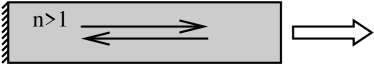
Figure 1: Schematic of a dielectric slab cavity of index $n_{0}$ and length $a$ with perfectly reflecting mirror at the origin.

Consider a dielectric medium of index $n=n_{0}$ which is uniform and infinite in the $y,z$ directions and extends from $x=0$ to $x=a$ in the $x$ direction. At $x=0$ it is terminated in a perfectly reflecting mirror and from $x=a$ to $\infty$ there is vacuum $(n=1)$. To clarify the difference between the CF states and the usual cold cavity resonances, first let us consider the quasi-bound states of such a resonator. These are defined as the solutions of

$$-\partial^{2}_{x}\varphi_{m}(x)=n_{0}^{2}\tilde{k}_{m}^{2}\varphi_{m}(x)$$ (30)

and the boundary condition (which can moved to the interface) $\partial_{x}\varphi_{m}(x=a)=i\tilde{k}_{m}\varphi_{m}(x=a)$. The complex eigenfrequencies of this problem are the solution of

$$\tan(n_{0}\tilde{k}_{m}a)=-in_{0}$$ (31)

which can be explicitly solved to yield

$$n_{0}\tilde{k}_{m}a=\pi(m+1/2)-i\frac{1}{2}\ln[\frac{n_{0}+1}{n_{0}-1}]\equiv n_{0}(q_{m}-i\kappa_{0})a,$$ (32)

where $m=1,2,\ldots,\infty$. Note that the imaginary part of the wavevector is always negative, as it should be, and in this case is constant, corresponding to the fixed transmissivity of a dielectric interface of index $n_{0}$ at normal incidence. Since these resonances are outgoing at infinity, each QB state varies as $e^{+i\tilde{k}_{m}x}\propto e^{+\kappa_{0}x}$ and grows exponentially at infinity as mentioned in the general discussion of QB states in the introduction.

Now consider the CF states; inside the medium they satisfy exactly the same equation and the continuity conditions at the dielectric interface are the same as well, but the CF state outside the dielectric satisfies the wave equation with a fixed external wavevector:

$$-\partial^{2}_{x}\varphi_{m}(x)=k^{2}\varphi_{m}(x),$$ (33)

and with the corresponding outgoing wave boundary condition, $\partial_{x}\varphi_{m}(x=a)=ik\varphi_{m}(x=a)$. This defines a family of basis states depending on the choice of the real external frequency $\omega=ck$. These eigenvalues satisfy the equation:

$$\tan(n_{0}k_{m}a)=-in_{0}\frac{k_{m}}{k}.$$ (34)

In the Appendix it is shown that this is a well-defined eigenvalue problem for any value of $k$ and the eigenvalues are always complex with negative imaginary part, similar to the usual QB states. But again, unlike the QB states, since $k$ is real, these states simply oscillate at infinity as $e^{ikx}$ and carry a constant outgoing flux.

One can see that if $k$ is chosen to be equal to $\tilde{q}_{m}$, the real part of the $m^{th}$ QB state wavevector, then the two eigenvalue conditions are almost the same in this vicinity. Note however that for every choice of the external wavevector $k$ there is an infinite set of CF eigenvalues. It is shown in the Appendix that from that infinite set there is one $m^{th}$ CF state with a wavevector very close to that of the corresponding QB state for $k=\tilde{q}_{m}$. Specifically, the difference between the wavevector of the $m^{th}$ QB state and the corresponding CF state is given by

$$n_{0}(q_{m}-\tilde{q}_{m})a=\frac{n_{0}\kappa_{0}}{k};\;\;\;\;n_{0}(\kappa_{m}-\kappa_{0})a=\frac{f(n_{0})}{(ka)^{2}},$$ (35)

where $f(n_{0})$ is a number of order unity depending on the index, $n_{0}$. Hence this difference is small in the semiclassical limit, $ka\gg 1$. Moreover both the CF and QB states are of the form $A\sin(k_{m}x)$ within the dielectric, so if their complex wavevectors are close, then the CF and QB states are almost identical in the medium. Thus we see that the standard cold-cavity resonances are almost equal to the lasing mode, but not exactly equal. Because the CF states are sines of complex wavevector they will oscillate and increase in amplitude within the medium (Fig. 2).

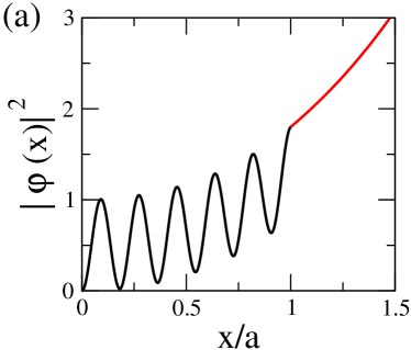
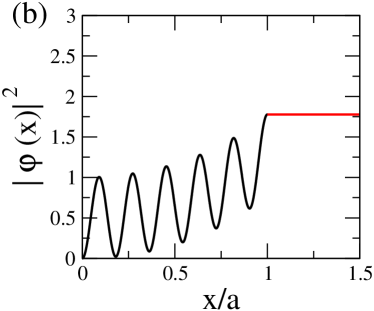
Figure 2: Solutions of the QB and CF state eigenvalue equations for a dielectric slab cavity with $n_{0}=2$. (a) A QB state at $\tilde{k}_{m}a=11.51917306-0.53647930i$. (b) A CF state at $k_{m}a=11.55535804-0.53100809i$ with external wavevector $ka=11.51917306$. Since the eigenvalues are almost the same the two solutions are almost identical within the cavity and show large amplification, but they differ qualitatively outside as the QB intensity grows exponentially while the CF intensity remains constant as required for a true lasing solution.

As noted in the general discussion, these CF states are not orthogonal when integrated within the medium. It is therefore useful to define adjoint CF states which satisfy the complex conjugate differential equation, and with the incoming boundary condition at infinity, $\partial_{x}\varphi_{m}(x=a)=-ik\varphi_{m}(x=a)$. It is easy to show that the eigenvalues $\bar{k}_{m}$ and eigenfunctions $\bar{\varphi}_{m}$ of this problem are the complex conjugates of the CF eigenvalues $k_{m}$, and eigenfunctions $\varphi_{m}$. In the Appendix it is confirmed that these functions satisfy the orthogonality relation $\int_{0}^{a}dx\varphi_{m}(x)\bar{\varphi}^{*}_{n}(x)=\int_{0}^{a}dx\sin(n_{0}k_{m}x)\sin(n_{0}k_{n}x)=\eta_{m}(\omega)\delta_{mn}$ and the normalization constant $\eta_{m}(\omega)$ is calculated. The biorthogonality of these functions follows from the boundary conditions at $x=a$.

III.3.2 Cylindrical CF states

The next case of interest is the case of a circular (2D) or cylindrical (3D) dielectric resonator of uniform index $n_{0}$ and radius $R$. The CF eigenvalues can be found by applying the conditions Eqs. (24) and (25) for the circle (2D) and cylinder (3D, solutions uniform in z-direction). Solutions can be labeled by their good angular momentum index in the z-direction, M, leading to a countably infinite sequence of eigenvalues for each value of M (which we will label by $m$). The states take the form

$$\varphi_{m}^{(M)}(r,\phi,\omega)=\begin{cases}J_{M}(n_{0}k_{m}r)\mbox{e}^{\pm iM\phi}&r<R\\ \frac{\mbox{J}_{M}(nk_{m}R)}{\mbox{H}_{M}^{+}(k_{m}R)}\,\mbox{H}_{M}^{+}(kr)\,\mbox{e}^{\pm iM\phi}&r>R\end{cases}$$ (36)

and the CF eigenvalue condition is found to be

$$\frac{\mbox{J}_{M}^{\prime}(n_{0}k_{m}R)\mbox{H}_{M}^{+}(kR)}{\mbox{H}_{M}^{+\prime}(kR)\mbox{J}_{M}(n_{0}k_{m}R)}=\frac{1}{n_{0}}\frac{k}{k_{m}}.$$ (37)

Note that this equation differs from that defining the QB states for this problem simply in that the corresponding QB eigenvalue condition would have $k_{m}$ appearing in the arguments of $H_{M}^{+}$, the external solutions, as well as in the arguments of $J_{M}$, the internal solutions.

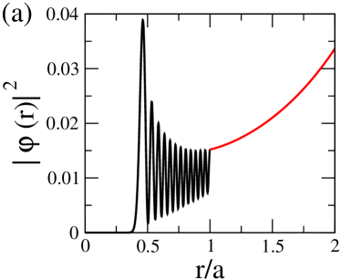
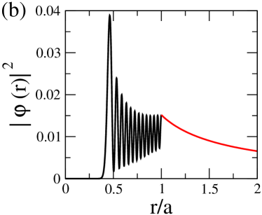
Figure 3: Solutions of the QB and CF state eigenvalue equations for a cylindrical dielectric resonator with $n_{0}=1.3$ and angular momentum quantum number $M=40$. (a) A QB state at $\tilde{k}_{m}R=71.17700357-0.74936509i$. (b) A CF state at $k_{m}R=71.19539070-0.74853902i$ with external wavevector $kR=71.17700357$. Again the two solutions are almost identical within the cavity; outside the QB solution grows while the CF solution decays as $1/r$ to conserve flux in 2D. The amplification of the solutions within the cavity is less obvious since both solutions have the usual peak at the caustic at $r/a\approx 0.45$; the decay away from this peak is actually slower going outwards then it would be for the cold cavity due to the amplification.

As for the slab resonator discussed above, if we choose $\omega=c\tilde{q}_{m}$, the real part of a specific QB state frequency, then we will find one CF eigenvalue close to the complex QB state eigenvalue, as long as the QB state itself has small imaginary frequency (high Q). A comparison of two such corresponding states is given in Fig. 3. Further analysis of the 2D case is given in the Appendix.

III.3.3 CF states for general shapes

The CF boundary conditions for a general dielectric body of arbitrary shape are still easily formulated in terms of outgoing spherical waves at infinity, since the object will appear point-like at arbitrary large distances. We simply require that the CF states satisfy the wave equation with index $n_{0}$ within the medium and that far away they have the form (in 2D)

$$\varphi_{m}(r\rightarrow\infty,\phi)=f_{m}(\phi)\frac{1}{\sqrt{r}}\mbox{e}^{ikr}.$$ (38)

In order to satisfy this boundary condition it will be necessary to solve the wave equation within the body by some method and continue it sufficiently far outside to a sphere or circle enclosing the body at which radius the interior solution can be connected to a superposition of outgoing waves with the wave-vector $k$. The situation is simplified if the dielectric body has a smooth shape and is not too far from spherical, in which case a Rayleigh (Bessel) expansion can be implemented within the cavity and can be matched to outgoing Hankel functions directly on the boundary specified by $R(\phi)$:

$$\varphi_{m}(r,\phi)=\begin{cases}\sum_{M}\alpha_{M}\mbox{J}_{M}(nk_{m}r)\mbox{e}^{iM\phi}\;\;\;&r<R(\phi),\\ \sum_{M}\gamma_{M}\mbox{H}_{M}^{+}(kr)\mbox{e}^{iM\phi}\;\;\;&r>R(\phi)\end{cases}$$ (39)

The continuity boundary conditions on the boundary can be easily cast into a secular equation and the eigenvalue condition replaced by a singularity condition. The method is then identical to that described in reference Tureci et al. (2005) for finding the QB states of such an asymmetric resonant cavity (ARC) except that the matrix $\cal{S}$ which appears from the matching conditions is slightly different. Two examples from implementing this method for CF states are shown in Fig. 4 below.

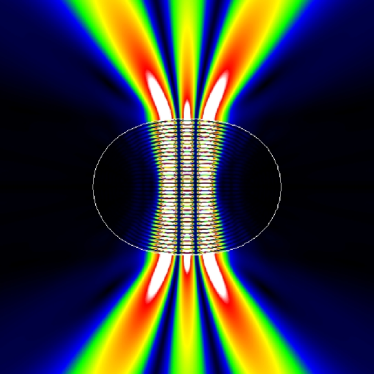
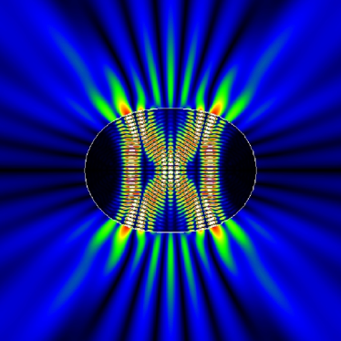
Figure 4: Gray scale plots of CF solutions for a dielectric cavity with a quadrupolar deformation $R(\phi)=R_{0}(1+\epsilon\cos 2\phi)$ at $\epsilon=0.16$ and an index of refraction $n=3.3$ at external wavevector $kR_{0}=20.0$. (Left) A bouncing ball mode at $k_{m}R_{0}=20.48417472-0.09782270i$ and (Right) a bowtie mode at $k_{m}R_{0}=19.71417046-0.040257141i$. Modes of the bowtie type were found to lase in the experiments of Ref. Gmachl et al. (1998).

IV Generalized multimode lasing equations

IV.1 Non-linear multimode equations

We now return to the formulation of the multi-mode lasing equations within the single-pole approximation to the Green Function. The outgoing lasing field $e(x,\omega)$ is only non-zero at the lasing frequencies; we approximate the Green function in the vicinity of $\omega=\Omega_{\mu}$ by the term arising from the nearest pole, i.e. $G(\bm{x},\bm{x}^{\prime}|\omega=\Omega_{\mu})\approx(c^{2}\varphi_{\mu}(\bm{x},\Omega_{\mu})\bar{\varphi}^{*}_{\mu}(\bm{x}^{\prime},\Omega_{\mu}))/(2n^{2}\omega_{a}(\Omega_{\mu}-\omega_{\mu}(\Omega_{\mu}))$. Equation (20) now takes the form:

$$a_{\mu}\left(1-i\tilde{D}_{0}\frac{1}{(-\delta\omega_{\mu}+i\kappa_{\mu})}\frac{\gamma_{\perp}}{(-i\Omega_{\mu}+\gamma_{\perp})}\int_{cavity}d\bm{x}^{\prime}\frac{\bar{\varphi}^{*}_{\mu}(\bm{x}^{\prime},\Omega_{\mu})\varphi_{\mu}(\bm{x}^{\prime},\Omega_{\mu})}{1+\sum_{\nu}g(\Omega_{\nu})|a_{\nu}|^{2}|\varphi_{\nu}(\bm{x}^{\prime},\Omega_{\nu})|^{2}}\right)=0$$ (40)

where $\tilde{D}_{0}$ is the scaled pumping rate given by

$$\tilde{D}_{0}=\frac{2\pi\omega_{a}g^{2}}{\hbar n^{2}\gamma_{\perp}}D_{0}$$ (41)

We are looking for lasing solutions to these equations, i.e. solutions where at least one $a_{\mu}\neq 0$ and positive. Since $a_{\mu}=0,\forall_{\mu}$ is always a solution for the steady-state equations, once we reach a pump level at which non-zero solutions exist, we must check their stability.

This can only be done by writing time-dependent equations for the CF state amplitudes $a_{\mu}(t)$ (analogous to the standard modal expansions) and determining the effect of a small deviation from the coexisting solutions with $a_{\mu}=0$ and $a_{\mu}\neq 0$. Previous work based on the standard theory finds Fu and Haken (1991) that whenever a solution with $a_{\mu}\neq 0$ exists, the $a_{\mu}=0$ solutions are unstable to small deviations, which then flow to the finite amplitude solution with the largest number of lasing modes. We assume this property for the current work and will explore this stability issue in subsequent work. Ruling out the identically zero solutions, and defining $I_{\nu}\equiv|a_{\nu}|^{2}$, the general non-linear multimode problem can be cast in the form

$$1+\frac{i(-\delta\omega_{\mu}+i\kappa_{\mu})(-i\Omega_{\mu}+\gamma_{\perp})}{\tilde{D}_{0}\gamma_{\perp}}=F_{\mu}(I_{\nu})$$ (42)

where

$$F_{\mu}(I_{\nu})\equiv 1-\int_{cavity}d\bm{x}^{\prime}\frac{\bar{\varphi}^{*}_{\mu}(\bm{x}^{\prime},\Omega_{\mu})\varphi_{\mu}(\bm{x}^{\prime},\Omega_{\mu})}{1+\sum_{\nu}g(\Omega_{\nu})I_{\nu}|\varphi_{\nu}(\bm{x}^{\prime},\Omega_{\nu})|^{2}},$$ (43)

and we must look for the solution with the maximum number of non-zero positive $I_{\nu}$. Note that the CF states $\varphi_{\mu}(\bm{x})$ in the definition of $F_{\mu}$ are understood to be evaluated for $\omega=\Omega_{\mu}$ and normalized to unity at this frequency. We will refer to the full non-linear form of the self-consistent equation as the non-linear Haken-Sauermann (NLHS) equations; these equations can be treated numerically and we will present results for the single and two-mode cases below.

IV.2 Generalized Haken-Sauermann equations

To treat the multi-mode case more simply and to make contact with the standard Haken-Sauermann treatment we now make the near threshold approximation for $F_{\mu}$ expanding the denominator of the integrand as $1/(1+\sum_{\nu}g(\Omega_{\nu})|a_{\nu}\varphi_{\nu}(\bm{x}^{\prime})|^{2})\approx 1-\sum_{\nu}g(\Omega_{\nu})|a_{\nu}\varphi_{\nu}(\bm{x}^{\prime})|^{2}$. We then arrive at the generalized (linear) Haken-Sauermann (GHS) equations for the modal intensities:

$$1+\frac{i(-\delta\omega_{\mu}+i\kappa_{\mu})(-i\Omega_{\mu}+\gamma_{\perp})}{\tilde{D}_{0}\gamma_{\perp}}=\sum_{\nu}g(\Omega_{\nu})A_{\mu\nu}I_{\nu}.$$ (44)

where the overlap matrix $A_{\mu\nu}$ is given by

$$A_{\mu\nu}=\int d\bm{x}^{\prime}\,\bar{\varphi}_{\mu}^{*}(\bm{x}^{\prime})\varphi_{\mu}(\bm{x}^{\prime})|\varphi_{\nu}(\bm{x}^{\prime})|^{2}.$$ (45)

In the limit in which $\gamma_{\perp}\gg\Omega_{\mu}$ and the frequency shift $\delta\omega_{\mu}\approx 0$ we recover the standard form of the HS equation (Eq. (1) above), with the important difference that the overlap matrix $A_{\mu\nu}$ is differently defined; it is complex and involves the integral of three outgoing CF states and one biorthogonal incoming state, whereas the usual HS equations $A_{\mu\nu}$ involves the squared moduli of two closed cavity states and is purely real. This new form allows us to determine iteratively the lasing frequency shifts in the multi-mode case, whereas the real approximation does not. A second difference is that in the usual HS equations the cavity widths $\kappa_{\mu}$ are put in by hand at this point, as the closed cavity states have zero width. In our approach the widths appear automatically as the imaginary parts of the complex wavevectors of the CF states. Finally we note that in this formulation the theory of interacting lasing modes can be seen to have some similarity to the theory of interacting electrons in quantum dots, as the overlap matrix $A_{\mu\nu}$ is similar to a mesoscopic two-body matrix element. When the resonator involved has complex (e.g. wave-chaotic) modes these matrix elements will fluctuate and depend sensitively on external parameters such as shape and pump profile. Concepts from random matrix theory and semiclassical quantum mechanics may be useful in analyzing these interactions; an example of this approach using the usual near threshold HS equations is the work of Misirpashaev and Beenakker Misirpashaev and Beenakker (1998).

V Solution of the generalized HS equations

V.1 Iterative method

Both the non-linear form (20) and linear form (44) of the generalized HS equations require a self-consistent iterative solution since the function $F_{\mu}(I_{\nu})$ in its exact and linearized form depends on the unknown lasing frequencies $\Omega_{\mu}$ as well as the unknown intensities $I_{\nu}$. Recall that the quantities $\delta\omega_{\mu}$ and $\kappa_{\mu}$ which appear explicitly in the NLHS and GHS equations are the difference between the lasing frequency $\Omega_{\mu}$ and the nearest CF state complex frequency $\omega_{\mu}(\Omega_{\mu})$; thus both of these quantities are determined by the real lasing frequencies. Therefore an initial ansatz for the lasing frequencies is required in order to begin the root search to determine the $\{I_{\nu}\}$. Conceptually the linear and non-linear cases are solved by similar iterative schemes, the only difference being that in the linear case (GHS) the root search becomes equivalent to inverting a linear system. In the linear case the solution must observe the constraint that $I_{\nu}\geq 0$ while in the non-linear case the positive roots, if they exist, have to be determined (as $I_{\nu}=0$ is always a solution).

At least two approaches are possible. One can start with the $N$ quasi-bound state frequencies which have real parts within a linewidth $\gamma_{\perp}$ of $\omega_{a}$ and use $\mbox{Re}\left[\omega_{\mu}^{qb}\right]\equiv\Omega_{\mu}^{qb}$ as the initial iterate for the real lasing frequencies. A second approach is to linearize the eigenvalue equation around the atomic frequency $\omega_{a}$, assuming that the imaginary parts of the CF frequencies don’t change rapidly so that one can use the imaginary parts determined by solving the CF eigenvalue condition at $\omega_{a}$ as a starting point for the iteration. Each of these approaches has advantages and can lead to a tractable scheme, as we will discuss below in the context of specific examples. We will describe the first approach here.

We first separate the real and imaginary parts of Eq. (44)

$$1-\frac{1}{D_{0}\gamma_{\perp}}\left[\delta\omega_{\mu}\Omega_{\mu}+\kappa_{\mu}\gamma_{\perp}\right] = \mbox{Re}\left[F_{\mu}\right]$$ (46)

$$-\delta\omega_{\mu}\gamma_{\perp}+\Omega_{\mu}\kappa_{\mu} = D_{0}\gamma_{\perp}\mbox{Im}\left[F_{\mu}\right]$$ (47)

where we have dropped the tilde on $D_{0}$. Our initial guess for the lasing frequencies is $\Omega_{\mu}^{(0)}=\Omega_{\mu}^{qb}$. The quantities $\delta\omega_{\mu},\Omega_{\mu},\kappa_{\mu},F_{\mu}$ in Eq. (46) are all functions of the true lasing frequencies $\Omega_{\mu}$. However we will approximate them by their values at the $\Omega_{\mu}^{(0)}$: let $\delta\omega_{\mu}^{(0)}=\mbox{Re}\left[\omega_{\mu}(\Omega_{\mu}^{(0)})\right]-\Omega_{\mu}^{(0)}$, $\kappa_{\mu}^{(0)}=-\mbox{Im}\left[\omega_{\mu}(\Omega_{\mu}^{(0)})\right]$, $F_{\mu}=F_{\mu}(\{\Omega_{\nu}^{(0)}\})\equiv F_{\mu}^{(0)}$; Eq. 46 then becomes

$$1-\frac{1}{D_{0}\gamma_{\perp}}\left[\delta\omega_{\mu}^{(0)}\Omega_{\mu}^{(0)}+\kappa_{\mu}^{(0)}\gamma_{\perp}\right]=\mbox{Re}\left[F_{\mu}^{(0)}(\{I_{\nu}\})\right].$$ (48)

This equation can be solved for the modal intensities $I_{\nu}^{(0)}$ by varying the pump power and looking for positive roots for different trial sets of lasing modes. In practice one easily finds the threshold for the first mode to lase and then increases the pump in steps above this.

Having determined the intensities, Eq. (46) yields an expression for the lasing frequencies by substituting $\Omega_{\mu}=\Omega_{\mu}^{(0)}+\delta\Omega_{\mu}$, $\delta\omega_{\mu}=\delta\omega_{\mu}^{(0)}-\delta\Omega_{\mu}$, $\kappa_{\mu}=\kappa_{\mu}^{(0)}$ and solving for $\delta\Omega_{\mu}$

$$\delta\Omega_{\mu}=\frac{\gamma_{\perp}(\delta\omega_{\mu}^{(0)}+D_{0}\mbox{Im}\left[F_{\mu}^{(0)}\right])-\kappa_{\mu}^{(0)}\Omega_{\mu}^{(0)}}{\gamma_{\perp}+\kappa_{\mu}^{(0)}}.$$ (49)

These equations yield the updated lasing frequencies $\Omega_{\mu}^{(1)}$ which can be reinserted into the equations to obtain higher iterations. We should note that Eqs. (48) and (49) are correct to O($\delta\Omega_{\mu}$) and O($\delta\Omega_{\mu}^{2}$) respectively, and we have neglected terms of O($\partial\omega_{\mu}/\partial\omega$) which can be shown to be small in the short wavelength limit. Thus Eqs. (48) and (49) are expected to converge rapidly with iteration number.

The equation for the frequency shifts is a generalization of well-known results for the single-mode case and the closed cavity. First note that for the closed cavity the function $F_{\mu}$ is real and doesn’t enter the imaginary part of the HS equations; hence the pump strength drops out. In addition, in a standard treatment the real frequency shift $\delta\omega_{\mu}^{(0)}$ is assumed to be zero since one begins with the cold cavity frequency, so one obtains:

$$\delta\Omega_{\mu}=\frac{-\kappa_{\mu}^{(0)}\Omega_{\mu}^{(0)}}{\gamma_{\perp}+\kappa_{\mu}^{(0)}}.$$ (50)

This gives the well known result that when the cavity width is large compared to the atomic relaxation rate one obtains $\delta\Omega_{\mu}=-\Omega_{\mu}^{(0)}\rightarrow\Omega_{\mu}=0$ i.e. lasing at the atomic frequency $\omega_{a}$; when $\kappa_{\mu}^{(0)}<<\gamma_{\perp}$ (the cavity mode is much narrower than the atomic linewidth) one obtains $\delta\Omega_{\mu}=-(\kappa_{\mu}^{(0)}/\gamma_{\perp})\Omega_{\mu}^{(0)}\rightarrow\Omega_{\mu}\approx\Omega_{\mu}^{(0)}=\mbox{Re}\left[\omega_{\mu}^{qb}\right]$, i.e. lasing at the cold cavity frequency. Our generalization shows that openness of the cavity introduces the pump strength into these equations and implies a change of the lasing frequencies with pump strength. This is a prediction of our theory which can in principle be tested experimentally.

V.2 Single mode solutions

V.2.1 Near-threshold behavior

The simplest solution of Eqs. (48) and (49) is the case where the electric field is oscillating at a single frequency $\Omega_{\mu}$. Then, we can solve Eqs. (48) and (49) straightforwardly for $I_{\mu}$ and $\Omega_{\mu}$:

$$I_{\mu}=\frac{1}{g(\Omega_{\mu}^{(0)})A_{\mu\mu}^{(0)}}\left(1-\frac{\kappa_{\mu}^{(0)}}{D_{0}}\right)$$ (51)

With uniform pumping this equation implies that the first mode to lase (and the only one in the single-mode approximation) is indeed the mode with the highest Q, corresponding to the CF state with the smallest value of its imaginary wavevector $\kappa_{\mu}$. (Of course, in a realistic scenario the laser typically will not remain single-mode for the whole range of pump rates $D_{0}$ and other modes can begin to oscillate). As noted above, unlike the closed cavity single-mode theory, for which the lasing frequency is independent of pump strength, in this case we find

$$\Omega_{\mu}=\frac{\gamma_{\perp}\omega_{\mu}^{(0)}+\gamma_{\perp}D_{0}g(\Omega_{\mu}^{(0)})\mbox{Im}\left[A_{\mu\mu}^{(0)}\right]I_{\mu}}{\gamma_{\perp}+\kappa_{\mu}^{(0)}}.$$ (52)

The first term in the numerator gives the “center of mass” formula for the lasing frequency discussed above, but the second term is proportional to $I_{\mu}$ and demonstrates that there is a frequency pulling or pushing effect even in the single-mode case which depends on the pump strength and on the imaginary part of the inverse mode volume, $A_{\mu\mu}^{-1}$. The generalization to multi-mode lasing is here trivial with the factor $\mbox{Im}\left[A_{\mu\mu}\right]I_{\mu}$ simply replaced by $\sum_{\nu}\mbox{Im}\left[A_{\mu\nu}\right]I_{\nu}$ (cf. Eq. (44)).

V.2.2 Far from threshold behavior

To generalize the above results to arbitrary pump rates we simply replace in Eqs. (48) and (49) $F_{\mu}$ by its exact expression

$$F_{\mu}=1-\int_{cavity}d\bm{x}^{\prime}\frac{\bar{\varphi}^{*}_{\mu}(\bm{x}^{\prime})\varphi_{\mu}(\bm{x}^{\prime})}{1+g(\Omega_{\mu})|\varphi_{\mu}(\bm{x}^{\prime})|^{2}I_{\mu}},$$ (53)

where it is understood that the CF states are calculated at the iteration frequency $\Omega_{\mu}=\Omega_{\mu}^{(i)}$.

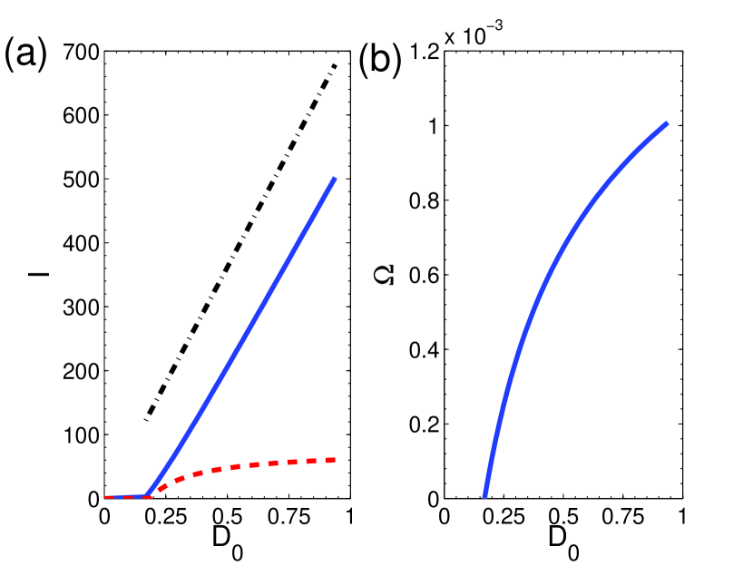
Figure 5: Single-mode single-pole solutions for the modal intensity vs. pump strength $D_{0}$ for a circular dielectric resonator with an index of refraction $n=2.0$ and gain-center at $\omega_{a}=50.0$. (a) Single-mode solution for the intensity $I$ of the mode with an angular momentum quantum number $M=40$ lying closest to the gain center. Dashed line: near-threshold solution, solid line: exact solution for modal intensities $I$ and dot-dashed line: far-from threshold approximation discussed in the text (plotted only for $I>120$). (b) Lasing frequency $\Omega$ as a function of the pump strength $D_{0}$. Note that $\Omega$ is measured from its value at the lasing threshold given by $\Omega_{0}=49.6668$ and the shift is towards the gain center frequency.

In Fig. 5 we show an example of the proposed iteration scheme for a dielectric resonator of circular cross-section. There are several observations we can make here. First of all, the intensity calculated from the near-threshold theory greatly underestimates the actual intensity at higher pump strengths $D_{0}$. As we shall further discuss below in Section V.3, this will have important consequences for mode competition in the multimode regime as the non-linear thresholds will be substantially different from those predicted by the near-threshold approximation. Second, as seen in Fig. 5(b) we now get a frequency shift that is power-dependent, with a non-linear dependence on the lasing intensities. This dependence is stronger the leakier the lasing mode. Third, the exact formula leads to an approximately linear dependence of the modal intensity $I_{\mu}$ on $D_{0}$. This linear dependence is termed ”saturation” in laser texts because it is much slower than the near threshold rise, but it is still a much stronger dependence than predicted by the near threshold HS theory. One can obtain a naive approximation for $I_{\mu}$ by replacing $1+g(\Omega_{\mu})|\varphi_{\mu}(\bm{x}^{\prime})|^{2}I_{\mu}$ in the denominator with $g(\Omega_{\mu})|\varphi_{\mu}(\bm{x}^{\prime})|^{2}I_{\mu}$, then

$$I_{\mu}=\left(\frac{\mbox{Re}\left[\Phi_{\mu}\right]}{g(\Omega_{\mu})\kappa_{\mu}}\right)D_{0}$$ (54)

where

$$\Phi_{\mu}=\int_{cavity}d\bm{x}^{\prime}\,\mbox{e}^{2i\phi_{\mu}(\bm{x}^{\prime})}$$ (55)

where $\phi_{\mu}(\bm{x}^{\prime})=-i\text{Arg}[\varphi_{\mu}(\bm{x}^{\prime})]$. For comparison, we plot the result of this expression in Fig. 5(b) (dot-dashed line). We see that this formula is qualitatively correct but overestimates the modal intensity.

V.3 Two-mode solutions

The numerical effort required to solve the linear and non-linear generalized HS equations for a non-trivial case, e.g. a dielectric cavity with fifty modes underneath the gain curve, is substantial. Moreover the interesting questions require varying the pump strength and the shape of the cavity. In earlier work we have done extensive calculations along these lines using the near threshold HS equations for the closed cavity and then using reasonable but uncontrolled approximations to evaluate the modal intensities outside the cavity Tureci and Stone (2005). The current generalized formalism gives us a method to evaluate emission directionality and output intensities correctly and without any approximations beyond the usual ones allowing a multi-mode solution. It also presents a formulation of the lasing equations valid away from the threshold, using the general function, $F(I_{\nu})$, defined in Eq. (43) above. A striking shortcoming of the near threshold approximation that we found in our earlier work Tureci and Stone (2005) is that it appears to overestimate greatly the number of lasing modes compared to the experimental observations Gmachl et al. (1998). Here we will not present realistic calculations on complex cavities using our generalized formalism; we defer such calculations to future work. Instead we present a simple comparison of the near-threshold and non-linear lasing solutions for the two-mode case, which confirms that the widely-used near threshold approximation can introduce a large quantitative error in the lasing thresholds and hence overestimates greatly the number of lasing modes for a given pump power in the complex dielectric cavity lasers we are studying. We solve Eq. (42) for two interacting modes of the dielectric cylinder (other modes which might also lase are neglected). In Fig. 6 and 7 we show the results. For mode 1, with the lower threshold, the near-threshold and non-linear calculation give the same threshold as they must ($D_{0}\approx 0.11$), and then deviate substantially well above threshold as we already saw in the previous section. Mode 2, which would have a threshold of $D_{0}\approx 0.18$ without mode competition has a threshold of $D_{0}\approx 0.25$ in the near threshold approximation, including the effects of mode competition, but has a correct threshold, taking non-linear effects into account, of $D_{0}\approx 0.41$. Hence we see that in the large interval $0.25<D_{0}<0.41$ the near-threshold theory predicts that two modes would be lasing and with comparable intensity, while the full theory predicts only one lasing mode. Moreover, because of this delay, when Mode 2 does begin to lase, its intensity lags mode 1 by an order of magnitude in contrast to the prediction of the near threshold analysis. We expect these discrepancies to be enhanced if there are many competing modes and many fewer modes to be lasing at a given pump power than predicted by the near-threshold theory. These issues will be explored in detail in future work.

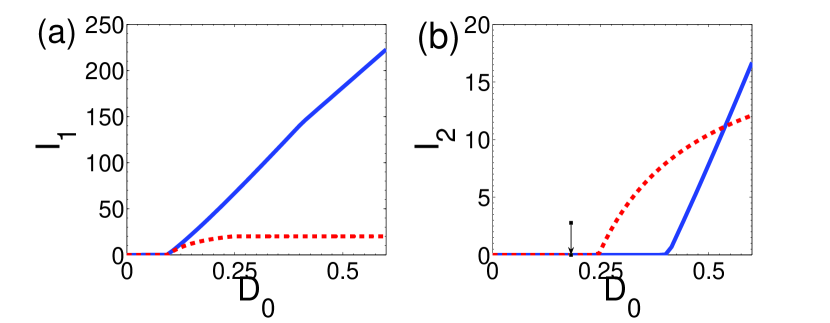
Figure 6: A single-pole two-mode solution for the modal intensities as a function of pump strength $D_{0}$ for a circular dielectric resonator with an index of refraction $n=2.0$ and gain-center at $\omega_{a}=20.0$. We have chosen $\gamma_{\perp}=50$ using effectively a flat gain curve. The two modes have the angular momentum quantum numbers $M_{1}=20$ and (b) $M_{2}=18$ respectively. The modal intensities $I_{1}$ and $I_{2}$ are given in (a) and (b). Solid lines denotes the exact solution, while we plot the near threshold approximate solution in dashed lines. The non-interacting thresholds are given by $D_{th}^{(1)}=0.1069$ and $D_{th}^{(2)}=0.1767$ (marked with vertical arrow in (b)). By definition modal interactions cannot change the first threshold, which is thus the same in the near-threshold and exact solution. However interactions dramatically modify subsequent thresholds; in this case the second threshold is increased to $D_{th}^{(2)}=0.2464$ in the near threshold approximation, but actually should be increased much more, to $D_{th}^{(2)}=0.4139$, based on the exact solution. This indicates that even taking modal interactions into account through the near-threshold approximation is inadequate and likely greatly overestimates the number of lasing modes at a given pump power.

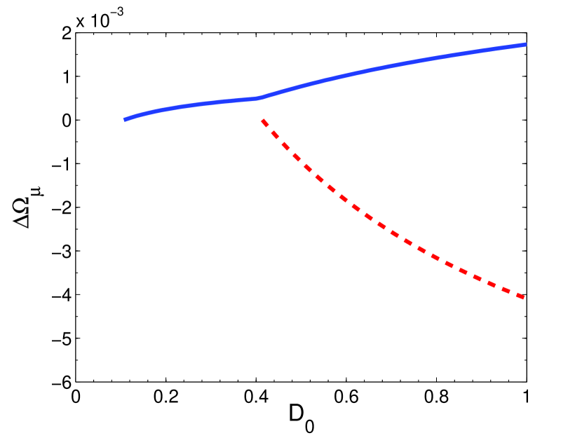
Figure 7: The corresponding laser frequency variation with pump power for the example in Fig. 6 as a function of pump strength $D_{0}$, for the exact solution. The frequencies of the two modes are measured with respect to their values at their respective lasing thresholds given by $\Omega_{1}=19.8584$ (full line) and $\Omega_{2}=20.3764$ (dashed line). Note that since the gain center is $\omega_{a}=20.0$ both modes are pulled towards the gain center.

VI Summary and Conclusions

We have reformulated semiclassical lasing theory to treat open cavities, with particular attention to complex and random lasers, for which the output power and directional emission patterns are not trivially found from knowledge of the internal modal intensities. We begin from the assumption that a steady-state multi-periodic lasing solution exists and is stable. A key idea is to formulate the theory in terms of the self-consistent linear response to the polarization described by an outgoing Green function. This yields a set of self-consistent integral equations for the lasing modes which can be solved by various means. The approach which is closest to conventional multi-mode lasing theory is to write a spectral representation of this Green function in terms of outgoing states with constant flux. For high Q cavities these states are similar but distinct from the usual resonances or quasi-bound states; they satisfy useful biorthogonality relations with adjoint functions. The Green function is then approximated by a single-pole near each lasing frequency implying the lasing mode is just an intensity $I_{\mu}$ times a single CF state. General and near-threshold equations then follow for these intensities $I_{\mu}$ and for the lasing frequencies $\Omega_{\mu}$. The near threshold equations are generalizations of the well known Haken-Sauermann equations derived for a closed cavity. These equations can account for the effects of mode competition and spatial hole-burning which are important but difficult to treat in complex cavity lasers. An iterative scheme was described for solving these equations and some illustrative results were given for the single-mode and two-mode case. The one and two-mode solutions indicate that the near-threshold approximation substantially overestimates the number lasing modes well above threshold and underestimates their output power.

In our view this approach clarifies the longstanding question of how to treat rigorously open cavities within semiclassical lasing theory. It now remains to apply this formalism to cases of interest: dielectric micro-cavity lasers of interesting shape, cavities with fully chaotic ray motion, and lasing from random media.

Appendix A Properties of the constant flux basis

In this Appendix we will explore the constant flux (CF) states, as defined in Sec. III.3.1. We investigate the analytically tractable cases of the 1D dielectric slab laser and the 2D cylindrical laser, and argue that the qualitative features of the solutions for these simple geometries should also hold for more general shapes. Here we focus on three properties of the CF basis. First, that for each high-Q QB state of the cavity there exists a single CF state with similar real and imaginary part and hence very similar behavior within the cavity (where they satisfy the same differential equation with just a slightly shifted eigenvalue). Second, we prove that all the CF states have eigenvalues with negative imaginary parts, corresponding to amplification of the wave within the cavity. Third, we confirm explicitly the biorthogonality of the two (outgoing and incoming) CF bases within the cavity for a general geometry.

A.1 Dielectric slab cavity

As stated in Sec. III.3.1, for a semi-infinite dielectric “slab” resonator the QB and CF eigenvalue equations are:

$$\tan{(n\tilde{k}_{m}a)}=-in$$ (56)

and

$$\tan{(nk_{m}a)}=-in\left(\frac{q_{m}-i\kappa_{m}}{k}\right)$$ (57)

Where $\tilde{k}_{m}\equiv\tilde{q}_{m}-i\tilde{\kappa}_{m}$ and ${k_{m}}\equiv q_{m}-i\kappa_{m}$ are the complex QB and CF wavenumbers, $a$ is the length of the slab, $n$ is the (possibly complex) index of refraction, and $k$ is the wavenumber corresponding to the external’ Fourier frequency. As in the main text we use tildes to denote quantities associated with the QB states, but we drop the subscript $0$ on the index of refraction. We also define the dimensionless quantities $x_{m}=nq_{m}a$, $y_{m}=-n\kappa_{m}a$, and $z=nka$. Using trigonometric identities, we can expand both equations into real and imaginary parts:

$$\frac{\cot{\tilde{q}_{m}}(1-\tanh^{2}{\tilde{\kappa}_{m}})}{\cot^{2}{\tilde{q}_{m}}+\tanh^{2}{\tilde{\kappa}_{m}}}=0$$ (58)

$$\frac{\tanh{\tilde{\kappa}_{m}}(\cot^{2}{\tilde{q}_{m}}+1)}{\cot^{2}{\tilde{q}_{m}}+\tanh^{2}{\tilde{\kappa}_{m}}}=-n$$ (59)

and

$$\frac{\cot{x_{m}}(1-\tanh^{2}{y_{m}})}{\cot^{2}{x_{m}}+\tanh^{2}{y_{m}}}=\frac{ny_{m}}{z}$$ (60)

$$\frac{\tanh{y_{m}}(\cot^{2}{x_{m}}+1)}{\cot^{2}{x_{m}}+\tanh^{2}{y_{m}}}=-\frac{nx_{m}}{z}$$ (61)

In the method used to solve the multimode laser equations presented in this paper, the Green’s function is approximated by a single pole, i.e. by a single CF state in the spectral representation of Eq. (29). We are therefore especially interested in finding solutions to the CF eigenvalue equation with real part close to the wavevector, k, appearing as a parameter in the CF eigenvalue equation. Furthermore, since we expect the real part of the QB mode frequencies to provide a first approximation to the actual lasing frequencies, we look for solutions to the CF eigenvalue equations with the external Fourier frequency set equal to the real part of a quasibound mode frequency. Equations (58)-(61) suggest that, for each QB mode with a sufficiently short wavelength, a corresponding CF solution exists with approximately the same eigenvalue, since in this limit $x=n\tilde{k}_{m}a$ is large. In that case the right hand side of (60) is small so that (60) is nearly identical to (58), and for $q_{m}\approx x$ equation (61) approaches (59).

The solution to Eqs. (58) and (59) was given in the text by equation (32), and equations (60) and (61) can be solved for $\tanh{y_{m}}$ and $\cot{x_{m}}$:

$$\tanh{y_{m}}=\frac{-(\cot^{2}{x_{m}}+1)\pm\sqrt{(\cot^{2}{x_{m}}+1)^{2}-4(nx_{m}/z)^{2}\cot^{2}{x_{m}}}}{2nx_{m}/z}$$ (62)

$$\cot{x_{m}}=\frac{(1-\tanh^{2}{y_{m}})\pm\sqrt{(1-\tanh^{2}{y_{m}})^{2}-4(ny_{m}/z)^{2}\tanh^{2}{y_{m}}}}{2ny_{m}/z}$$ (63)

Note that in order to self-consistently choose solutions to (62) and (63) which are close to QB solutions, we must select the minus signs in both equations. We now expand (60) in the small difference $\delta q_{m}=q_{cf}-q_{qb}$:

$$\frac{\delta x_{m}(1-1/n^{2})}{1/n^{2}}\approx-\frac{n}{z}y_{m}$$ (64)

Assuming that $\delta y_{m}$ is, at most, first order in the small parameter $z^{-1}$, we can replace $y_{m}$ with $\tilde{\kappa}_{m}$, leading to:

$$\delta x_{m}(n^{2}-1)\approx-\frac{n}{z}\tilde{\kappa}_{m}$$ (65)

Or, using the expression for $\kappa_{0}$ from Eq. (32) and the definitions of $x_{m}$ and $z$:

$$\delta q_{m}\approx\frac{\ln{[\frac{n+1}{n-1}]}}{2(n^{2}-1)}\frac{1}{na^{2}k}$$ (66)

We see the difference between real part of the CF resonance and the external frequency is small when (1) the external frequency is set near the real part of a QB resonance and (2) the semiclassical parameter $z^{-1}$ is small. To find an approximation for $\kappa_{m}$, as well as to justify the approximation used in deriving (66) that $y_{m}\approx\tilde{\kappa}_{m}$, we next expand (62) to second order in $\delta q_{m}^{-1}$ and $x^{-1}$. After some manipulation we obtain:

$$\delta\kappa_{m} \approx-\frac{1}{2(n^{2}-1)^{2}}\ln{[\frac{n+1}{n-1}]}\left(1+\frac{\ln{[\frac{n+1}{n-1}]}}{2}\right)\frac{1}{na^{3}k^{2}}$$

$$=\frac{f(n)}{(ka)^{2}}\frac{1}{a}$$ (67)

Which is the result quoted in Section III.3.1. Thus we see that $\delta q_{m}$ is first order and $\delta\kappa_{m}$ is second order in $z^{-1}$. Fig. (8) shows that the approximation used here agrees well with the numerically evaluated results for the difference between the QB and the nearest CF wavevector.

\psfrag{A}{$\frac{\tilde{q}_{m}-q_{m}}{\tilde{q}_{m}}$}\psfrag{B}{$\tilde{q}_{m}$}\psfrag{C}{$\frac{\tilde{\kappa}_{m}-\kappa_{m}}{\tilde{\kappa}_{m}}$}\psfrag{D}{$\ln{\tilde{\kappa}_{m}}$}\psfrag{E}{$\tilde{q}_{m}$}\includegraphics[width=433.62pt]{DxDycombo.eps}

Figure 8: The difference between the CF and QB eigenvalues for a 1D dielectric slab resonator, as a function of the real part of the QB eigenvalue. (a) The fractional difference between the real part of the eigenvalues, and (b) the fractional difference between the complex parts. In both plots, the triangles represent the actual difference, found numerically, which is compared to the linear approximation, Eq. (67), derived in the text and represented by the solid curves.

A.2 Cylindrical dielectric cavity

It is well known that for a cylindrical cavity, there exist whispering gallery mode solutions to the QB eigenvalue equation that have very small widths, $\tilde{\kappa}_{m}$. Moreover, it is these modes which will dominate lasing emission from dielectric cylinder lasers. In this section we show that there exist corresponding solutions to the CF eigenvalue equations close to these QB solutions. Specifically, the difference between the CF and QB lifetimes is proportional to a small factor times the QB lifetimes; hence these CF and QB states have almost identical lifetimes.

The QB eigenvalue equation for a cylindrical resonator is:

$$\frac{d}{dr}J_{M}(n\tilde{k}_{m}R)/J_{M}(n\tilde{k}_{m}R)=\frac{d}{dr}H^{(+)}_{M}(\tilde{k}_{m}R)/H^{(+)}_{M}(\tilde{k}_{m}R)$$ (68)

Within the regime of interest where the modes are well trapped (and the index of refraction is not too small), we can approximate the Hankel and Bessel functions appearing in this equation by the Debye approximations Abramovitz and Stegun (1972). Define $\tanh{\alpha}=\sqrt{1-(\tilde{k}_{m}R/M)^{2}}$ and $\tan{\beta}=\sqrt{(n\tilde{k}_{m}R/M)^{2}-1}$. In terms of these variables, the Debye approximations are:

$$J_{M}(k_{m}R)=\frac{e^{M(\tanh{\alpha}-\alpha)}}{\sqrt{2\pi M\tanh{\alpha}}}$$ (69)

$$Y_{M}(k_{m}R)=-\frac{e^{-M(\tanh{\alpha}-\alpha)}}{\sqrt{\frac{1}{2}\pi M\tanh{\alpha}}}$$ (70)

$$J_{M}(nk_{m}R)=\frac{\cos{(M\tan{\beta}-M\beta-\frac{\pi}{4})}}{\sqrt{\frac{1}{2}\pi M\tanh{\alpha}}}$$ (71)

$$Y_{M}(nk_{m}R)=\frac{\sin{(M\tan{\beta}-M\beta-\frac{\pi}{4})}}{\sqrt{\frac{1}{2}\pi M\tanh{\alpha}}}$$ (72)

Note that in the regime in which these approximations are valid, we can ignore the r-dependence outside the exponent when we evaluate its derivatives, so that the eigenvalue equation is approximately:

$$\tan{\beta}\tan{\lambda}\approx\tanh{\alpha}\frac{e^{\mu}+2ie^{-\mu}}{e^{\mu}-2ie^{-\mu}}$$ (73)

where we have defined $\lambda=M(\tan{\beta}-\beta)-\frac{\pi}{4}$ and $\mu=M(\tanh{\alpha}-\alpha)$. By expanding in the small quantity $\tilde{\kappa}_{m}$ and neglecting $e^{\mu}$ compared to $e^{-\mu}$ (which is valid for well trapped modes), we can derive an approximate expression for $\tilde{\kappa}_{m}$:

$$\tilde{\kappa}_{m}\approx\frac{M\tanh{\alpha}}{n^{2}a^{2}\tilde{q}_{m}(n^{2}-1)}e^{2\mu}.$$ (74)

A similar, but not identical, result was obtained by Nöckel Nöckel (1997), where it was pointed out that the small factor $e^{2\mu}$ could be interpreted as the exponential decay factor due to tunneling.

\psfrag{A}{$\frac{\tilde{q}_{m}-q_{m}}{\tilde{q}_{m}}$}\psfrag{B}{$\tilde{q}_{m}$}\psfrag{C}{$\frac{\tilde{\kappa}_{m}-\kappa_{m}}{\tilde{\kappa}_{m}}$}\psfrag{D}{$\ln{\tilde{\kappa}_{m}}$}\psfrag{E}{$\tilde{q}_{m}$}\psfrag{F}{$\frac{\kappa_{m}-\tilde{\kappa}_{m}}{\tilde{\kappa}_{m}}$}\includegraphics[width=433.62pt]{YDYcombo.eps}

Figure 9: (a) The log of the imaginary part of the QB resonance eigenvalue for a cylindrical resonator with $n_{0}=2$, plotted against the real part of the eigenvalue; triangles represent numerical results compared to the analytic approximation of Eq. (74). (b) The fractional difference between the CF and QB lifetimes versus the real part of the QB eigenvalue for the same resonator. Stars are numerical results, solid line the approximation of Eq. (75). We have plotted the sequence corresponding to angular momentum $M=50$.

The eigenvalue equation for CF modes in a cylindrical resonator has the same form as Eq. (68) above for QB states except that the functions $\alpha$, $\beta$, $\lambda$ and $\mu$ appearing in the CF equation are evaluated at different arguments. Explicitly, $\lambda$ and $\beta$ are evaluated at $k_{m}R=\tilde{k}_{m}R+\delta(k_{m}R)$, whereas $\mu$ and $\alpha$ are evaluated at the external Fourier frequency, which we have set equal to $\tilde{q}_{m}$. We can then expand in the small quantities $\delta(k_{m}R)$ and $\tilde{\kappa}_{m}$. To first order, the imaginary part of this equation yields:

$$\delta(\kappa_{m})\approx\frac{\tilde{\kappa}_{m}}{M(n^{2}-1)\tanh{\alpha}},$$ (75)

where it is understood that $\tanh{\alpha}$ is evaluated at $\tanh{\alpha}=\sqrt{1-(\frac{\tilde{k}_{m}R}{M})^{2}}$ Note that in the semiclassical regime whispering gallery modes have a high M value, so the difference between the lifetimes for the CF and QB mode is a small factor times the already small QB lifetime $\tilde{\kappa}_{m}$.

A.3 General argument that $Im(k_{m})=-\kappa_{m}<0$

We were able to show above explicitly that for the CF eigenvalue closest to the corresponding QB state eigenvalue, $\kappa_{m}>0$ for both the 1D slab laser and the 2D cylindrical laser. Here we show that this result holds generally for all CF eigenvalues and for arbitrary geometries. This is important because the exact CF Green function involves all CF eigenvalues and it would be unphysical for it to have poles in the positive imaginary plane.

The equation satisfied by the CF states is:

$$\nabla^{2}\varphi(\bm{x})=\left\{\begin{array}[]{ll}n^{2}k_{m}^{2}\varphi(\bm{x})&\mbox{(inside)}\\ k^{2}\varphi(\bm{x})&\mbox{(outside)}\end{array}\right.$$ (76)

We define a vector flux as $\bm{f}=\frac{1}{2i}(\varphi^{*}\bm{\nabla}\varphi-\varphi\bm{\nabla}\varphi^{*})$. The outgoing wave boundary conditions, as expressed in the main text by equation (24), imply that if we integrate the radial component of $\bm{f}$ over increasingly larger spheres S (or circles in the 2D case) with origin within the cavity, the value of this integral approaches a positive constant proportional to $k$:

$$\int_{S}\bm{f}\cdot\bm{dA}\longrightarrow k\int|\varphi(\phi)|^{2}d\phi$$ (77)

Note that $\bm{\nabla}\cdot\bm{f}$ vanishes outside the cavity, whereas inside it is equal to $-n^{2}\varphi\varphi^{*}Im(k_{m}^{2})=2n^{2}|\varphi|^{2}q_{m}\kappa_{m}$. By using the divergence theorem and the CF equation we can also write this integral as:

$$\int_{S}\bm{f}\cdot\bm{dA}=\int_{Int(S)}\bm{\nabla}\cdot\bm{f}dV=2n^{2}q_{m}\kappa_{m}\int_{cavity}n^{2}|\varphi|^{2}d\bm{x}$$ (78)

Comparing equations (77) and (78) we can see that in order to satisfy (77), which follows from the outgoing wave boundary condition, we must have $\kappa_{m}>0$.

A.4 Biorthogonality of incoming and outgoing CF states

Consider a solution to the CF eigenvalue equation $\varphi_{m}$ with eigenvalue $k_{m}$, along with an adjoint solution $\overline{\varphi}_{n}$ with eigenvalue $k_{n}^{*}$. Using the fact that these two functions satisfy the eigenvalue equations (22) and (26), respectively, we have:

$$n_{0}^{2}(k_{n}^{2}-k_{m}^{2}) \int_{cavity}d\bm{x}\,\overline{\varphi}^{*}_{n}\varphi_{m}$$

$$=\int_{cavity}d\bm{x}\,\left(\overline{\varphi}^{*}_{n}\nabla^{2}\varphi_{m}-\varphi_{m}\nabla^{2}\overline{\varphi}^{*}_{n}\right)$$

$$=\int_{boundary}(\overline{\varphi}^{*}_{n}\bm{\nabla}{\varphi_{m}}-\varphi_{m}\bm{\nabla}\overline{\varphi}^{*}_{n})\cdot d\bm{A}$$ (79)

Where the last integral is over the surface of the cavity boundary. Outside the cavity we have $\bm{\nabla}\cdot(\overline{\varphi}^{*}_{n}\nabla{\varphi_{m}}-\varphi_{m}\nabla\overline{\varphi}^{*}_{n})=0$, so we can in fact replace the integral over the cavity boundary with an integral over a large sphere $S$ inclosing the cavity. We can then invoke the outgoing/incoming wave boundary conditions to evaluate the surface integral explicitly:

$$\int_{S}(\overline{\varphi}^{*}_{n} \bm{\nabla}{\varphi_{m}}-\varphi_{m}\bm{\nabla}\overline{\varphi}^{*}_{n})\cdot d\bm{A}$$

$$\longrightarrow\int_{S}(ik\overline{\varphi}^{*}_{n}{\varphi_{m}}-ik\varphi_{m}\overline{\varphi}^{*}_{n})\cdot d\bm{A}=0$$ (80)

For the case $k_{n}\neq k_{m}$, equations (79) and (80) therefore imply:

$$\int_{cavity}d^{3}x\overline{\varphi}^{*}_{m}\varphi_{n}=0$$ (81)

It should be noted that, although the CF functions are defined to exist both inside and outside the cavity, the inner product is defined by an integral over the cavity interior only. The biorthogonality of the CF states is therefore determined completely by their behavior within the cavity and at its boundary; we merely use the behavior of the CF functions at infinity to show that the surface term in equation (79) vanishes whenever the CF states satisfy the outgoing/incoming boundary conditions.

We can check the biorthogonality of the CF states explicitly for the case of the dielectric slab cavity, and also calculate the normalization factor $\eta_{m}(\omega)$ defined in equation (28). In the cavity interior, we have

$$\varphi_{n}(x)=\sin(n_{0}k_{n}a)$$ (82)

and

$$\overline{\varphi}^{*}_{m}=\sin(n_{0}k_{m}a)$$ (83)

Using the trigonometric identity $\sin(s)\sin(t)=\frac{1}{2}(\cos(s-t)-\cos(s+t))$, we can write the inner product (for the case $m\neq n$) as:

$$\int_{0}^{a}\sin(n_{0}k_{n}a)\sin(n_{0}k_{m}a)dx$$

$$=\frac{\cos(n_{0}k_{n}a)\cos(n_{0}k_{m}a)}{2n_{0}}\left(\frac{\tan(n_{0}k_{n}a)-\tan(n_{0}k_{m}a)}{k_{n}-k_{m}}-\frac{\tan(n_{0}k_{n}a)+\tan(n_{0}k_{m}a)}{k_{n}+k_{m}}\right)$$

$$=0$$ (84)

Where we have used the eigenvalue equation (57). The normalization is:

$$\int_{0}^{a}\sin^{2}(n_{0}k_{n}a)dx=\frac{a}{2}\left(1-\frac{\sin 2(n_{0}k_{n}a)}{2(n_{0}k_{n}a)}\right)=\eta_{m}(\omega)$$ (85)