Phonons and Conduction in Molecular Quantum Dots: Density Functional Calculation of Franck-Condon Emission Rates for bi-fullerenes in External Fields

Abstract

We report the calculation of various phonon overlaps and their corresponding phonon emission probabilities for the problem of an electron tunneling onto and off of the buckyball-dimer molecular quantum dot $C_{72}$, both with and without the influence of an external field. We show that the stretch mode of the two balls of the dumbbell couples most strongly to the electronic transition, and in turn that a field in the direction of the bond between the two $C_{36}$ balls is most effective at further increasing the phonon emission into the stretch mode. As the field is increased, phonon emission increases in probability with an accompanying decrease in probability of the dot remaining in the ground vibrational state. We also present a simple model to gauge the effect of molecular size on the phonon emission of molecules similar to our $C_{72}$ molecule, including the experimentally tested $C_{140}$. In our approach we do not assume that the hessians of the molecule are identical for different charge states. Our treatment is hence a generalization of the traditional phonon overlap calculations for coupled electron-photon transition in solids.

I Introduction

Physics is full of examples of phonon-coupled quantum tunneling events. A classic example from the 1960s is the work done with trapped-electron color centers in the lattices of the alkali-halides schulman . More modern examples include the study of how the mobility of interstitials in metals is modulated by coupling of the defect to the resulting distortion of the surrounding lattice flynn and the study of how the inter-chain hopping by polarons is affected by phonon interactions conwell2 . In these studies and others, the frequencies before and after the transition were assumed to be unchanged and only the coordinate about which the harmonic potential is centered shifts. Here, our use of the word phonon, traditionally used for plane-wave-like solutions in periodic crystals, for vibrational normal mode is in the same spirit in this context for which we use the term quantum dot, a macroscale object, for molecule.

Over the past several years, several experiments and theoretical studies braig ; mitra ; schoeller have been done where single molecules have been used as the medium for vibration-assisted tunneling. Some recent experimental examples are measurements done with scanning tunnel microscopes ho ; stipe , studies of single hydrogen molecules in mechanical break junctions smit , and the investigations that have directly motivated this work, the three-terminal single molecule transistor experiments park1 ; park2 where a single molecule is deposited between two leads and is subjected to both a source-drain and gate bias. This is done in the Coulomb blockage regime, where the bias is tuned so that sequential transport can occur and a differential conductance graph can be plotted. In many of these differential conductance graphs, in addition to the main lines due to the change in the charge state of the molecule, there are a series of sidebands thought to be caused by the coupling of the electron to the vibrational modes of the molecule.

In this paper, we present a general theory for these vibrational overlaps where the vibrational modes of both the initial and final electronic states of the molecule are considered. Charge dependent hessians and anharmonic potentials in the context of single molecule transistors have been considered previously KV05 ; WN05 where the molecule is assumed to have one dominant mode in each electronic state. In the field of chemical spectroscopy, this topic has been addressed N01 through a general consideration of the Franck Condon factors with Duschinsky rotation D37 and its refinements KRLC93 ; CDLW98 , which allows for different frequencies and eigenvectors between different charged states. Our paper considers a realistic model of an N-atom molecule with 3N possible modes (for example, the bi-fullerene $C_{72}$ with $216$ possible modes, see figure (1)) and allows the calculation of experimental scenarios by combining our formulation with results from existing quantum chemistry packages.

Figure 1: $C_{72}$ with 19 meV stretch mode indicated

Spectroscopy has long been utilized as a tool in both chemistry and physics to study the properties and structure of atoms and molecules. Different types of spectroscopy are used for different aims; optical spectroscopy for example studies the interaction of electromagnetic radiation with the sample while this paper addresses differential tunneling spectroscopy. Franck-Condon factors serve as a very good tool for analyzing the absorption and emission band intensities corresponding to vibrational levels in atoms and molecules schatz . Over the years, many such molecular vibrational spectra have been calculated and cataloged using Franck-Condon factors coon ; herzberg . Single molecule transistors offer an opportunity to apply the Franck-Condon principles to a new system. Because we are dealing with single molecules, we can calculate (using quantum chemistry packages) the full vibrational profile of both the initial and final electronic states of the molecule, and thus calculate the Franck-Condon intensities generally.

Franck was the first to postulate that an electronic transition can be accompanied by a vibrational excitation using classical arguments franck . Condon later duplicated the argument using quantum mechanics and the Born-Oppenheimer approximation condon . According to Condon, the intensity of a particular transition can be determined by calculating the transition dipole moment. The electronic component can be factored out, leaving the square of the phonon overlap to modulate the total transition.

In section II, we set up our Hamiltonian. IN section III, we outline our version of the calculations of the phonon overlap calculations iincluding the ’Duschinsky rotation’. In section IV, we outline our DFT numerical methods. Section VI calculates the zero-field overlaps. Section VII addresses the overlaps in a field. Section VIII introduces a simple two-ball and spring model for the behavior of the stretch mode overlap in the presence of a field. Section IX makes contact with $dI/dV$ measurements of the entire spectrum and section X concludes.

II The Hamiltonian

The Hamiltonian for the molecular dot looks like, in a mixed first and second quantized formulation:

$$H=H_{1}+H_{2}+H_{3}$$ (1)

where $H_{1}$, $H_{2}$, and $H_{3}$ are given by the following:

$$H_{1}=\left[\sum_{k}\epsilon_{k}c^{l{\dagger}}_{k}c^{l}_{k}+\sum_{k}\epsilon_{k}c^{r{\dagger}}_{k}c^{r}_{k}+\epsilon_{d}c^{\dagger}_{d}c_{d}\right]$$ (2)

$$H_{2} = {1\over{2}}{\bf{p}^{\dagger}\mathsf{M}^{-1}\bf{p}}$$ (3)

$$+ (1-c^{\dagger}_{d}c_{d})\left[1/2(\bf{x}-{{\bf r}_{1}})^{\dagger}\mathsf{K_{1}}(\bf{x}-{{\bf r}_{1}})\right]$$ (4)

$$+ c^{\dagger}_{d}c_{d}\left[1/2(\bf{x}-{{\bf r}_{2}})^{\dagger}\mathsf{K_{2}}(\bf{x}-{{\bf r}_{2}})\right]$$ (5)

$$H_{3}=\sum_{k}T^{l}_{k}(c^{l{\dagger}}_{k}c_{d}+c^{\dagger}_{d}c^{l}_{k})+\sum_{k}T^{r}_{k}(c^{r{\dagger}}_{k}c_{d}+c^{\dagger}_{d}c^{r}_{k})$$ (6)

Here we do not incorportate explicit terms for spin and charging effects because we’re focused on sequential tunneling events where only one elextron is on the dot at a time. Terms like the Coulomb effect in equation (11) below, we disregard in our expression. Equation (2) describes the electronic component involving the left and right leads and the dot, equation (6) describes the tunneling component, and equation (3) are the phonon states. Here $\bf{p}$ is the $3N$-component vector for the momentum of the N-atom molecule, $\mathsf{M}$ is the mass matrix (diagonal entries giving the masses of the different nuclei in groups of three), $\bf{x}$ is the $3N$-dimensional vector for the atomic coordinates of the molecule, $\bf{r_{1}}$ and $\bf{r_{2}}$ are the $3N$-dimensional vectors for the minimum energy configurations of the inital and final electronic states, and $\mathsf{K_{1}}$ and $\mathsf{K_{2}}$ are the quadratic forms giving the energy near $\bf{r_{1}}$ and $\bf{r_{2}}$. The $1$ and $2$ indices reference the charge state of the molecule. In our transition, the $1$ index refers to the molecular state with smaller charge, and the $2$ index refers to the higher charge state. $T^{l/r}_{k}$ is the tunneling matrix where the superscripts $l$ and $r$ specifies the left or right lead. Finally, $c^{\dagger}$ and $c$ are creation and destruction operators, respectively, for electrons. An external force $\bf{f}$ on the atomic coordinates shifts the ground state configuration: e.g., $\bf{r_{2}}=\bf{r^{(0)}_{2}}+\mathsf{K_{2}}^{-1}\bf{f}$.

Although the phonon states can also be expressed in second quantized form via the creation and annihilation operators for bosonic particles $a^{\dagger}$ and $a$, we chose to express them in first quantized form to facilitate the calculation of the 3N-dimensional overlap integrals between different vibrational states of our initial and final molecule.

III Phonon Overlap Integrals

In regarding our problem, we are considering the case of incoherent tunneling, where one electron is tunneling on or off the molecular quantum dot at a time. We also assume that the molecule has time to relax to its minimum energy configuration in between tunneling events such that all phonon excitations decay before the next tunneling event. In recent experiments leroy , long phonon lifetimes extending at least fifty times beyond the lifetimes observed in Raman spectroscopy have been measured for experiments on suspended carbon nanotubes. However, the authors note that the lack of coupling to a substrate may account for this increase. In other experiments ho , the experimental setup was arranged to increase the lifetime of the electron compared to the phonon, allowing for observation of transient vibronic levels. For our calculation, we presume that low currents and strong phonon coupling between molecule and leads ensures vibrational relaxation between electron tunneling events.

Secondly, we assume the Born-Oppenheimer approximation where the total wave function is described by $|\Psi(z,x)\rangle=|\varphi_{x}(z)\phi(x)\rangle$, where $x$ labels the nuclear coordinates as above, and $z$ labels the electron coordinates. Strictly speaking, the ground-state electron wave function depends parametrically on the nuclear positions $x$. Based on geometric optimization calculations, we know the atomic fluctuations $\delta x$ are on the order of picometers, so we can safely assume $\phi_{x}(z)\approx\phi(z)$ and hence factor our wavefunction into a purely electronic component and a purely nuclear component. The transition then is given by the following matrix elements where $T$ is given by (6):

$$T_{fi} = \langle\Psi_{f}(z,x)|T|\Psi_{i}(z,x)\rangle$$ (7)

$$= \langle\varphi^{i}(z)\phi^{i}(x)|T|\varphi^{f}(z)\phi^{f}(x)\rangle$$ (8)

$$= \langle\varphi^{f}(z)|T|\varphi^{i}(z)\rangle\langle\phi^{f}(x)|\phi^{i}(x)\rangle$$ (9)

Following the Landauer approach landauer ; buttiker ; Beenakker2 and using Fermi’s Golden Rule to give us a transition probability, we can find the conductance. Sequential tunneling in the Coulomb Blockade regime is assumed  Beenakker for the case where the quantum dot has energy levels given by $E_{p}$ (For us, $E_{p}$ will represent one of many energy eigenstates with both a change in electron charge and the excitation of one or more vibrational modes). The formula for the conductance is then found to be:

$$conductance = {e^{2}\over{kT}}\sum_{p}\sum_{N}\Big{\{}{\Gamma^{l}_{p}\Gamma^{r}_{p}\over{\Gamma^{l}_{p}+\Gamma^{r}_{p}}}P_{eq}(N)F_{eq}(E_{p}|N)$$ (11)

$$\times[1-f(E_{p}+U(N)-U(N-1)-E_{F})]\Big{\}}$$

where $\Gamma^{l/r}_{p}$ is the tunneling rate from the dot electron energy level $p$ to the left/right leads, $N$ is the number of electrons in the dot before the tunneling event, $U(N)$ is the charging energy for $N$ electrons on the dot, $F_{eq}(E_{p}|N)$ is the conditional probability in equilibrium that the level p is occupied given that the quantum dot contains $N$ electrons, $E_{F}$ is the chemical potential of the leads, and $P_{eq}(N)$ is the probability that the quantum dot has $N$ electrons in equilibrium. In addition, the electrons in the leads are in the Fermi distribution $f(E)$.

Since tunneling rates depend exponentially on separation, the tunneling rate through one of the leads, say the right one, is often much smaller than the other, with the smaller rate acting as the bottleneck, ${\Gamma^{l}_{p}\Gamma^{r}_{p}\over{\Gamma^{l}_{p}+\Gamma^{r}_{p}}}\sim\Gamma^{r}_{p}$. Hence the dependence of $\Gamma^{r}_{p}$ on the final state $p$ determines the variation of the conductance with energy. This tunneling rate is proportional to $|T_{fi}|^{2}$, where $|T_{fi}|$ is given by (7). For a given electronic transition $\varphi^{i}$ to $\varphi^{f}$, assuming (at the low temperatures of these experiments) that the initial molecular state has no phonon excitations, the dependence of this matrix element on the final phonon state is given primarily by the phonon overlap integrals in equation (7), and hence

$$G\propto\Gamma^{r}_{p}\propto\sum_{\epsilon_{F}\leq eV}|\langle\phi^{f}(x)|\phi^{i}(x)\rangle|^{2}.$$ (12)

The linear conductance given in equation (12) is dependent only on the ground state since the excitation of phonons is related to the applied bias difference across the molecule. As each threshold step in bias is crossed, new possible pathways are accessible and the squares of their overlaps must be added to the expression.

This phonon overlap integral is the quantity of interest since it modulates the total transition rate. Its value is a measure of the probability of occurrence of a particular transition between the initial vibrational state of the initial charge state (assumed to always be the ground state) and the final vibrational state of the final charge state. This quantity will suppress the total transition rate matrix element, leading to less intensity in the line. Summing over final states yields 1 GS88 :

$$\sum_{f}|\langle\phi^{f}(x)|\phi^{i}(x)\rangle|^{2}=1$$ (13)

with the individual terms representing the probability decomposition of the initial state in the eigenstates of the final potential. Hence the weight of the original transition is spread among the phonon excitations.

III.1 Normal modes and phonon wavefunctions

In 3N dimensions, the phonon Hamiltonian for the initial charge state is:

$$H={1\over{2}}{\bf{p}}^{\dagger}\mathsf{M}^{-1}{\bf{p}}+{1\over{2}}({\bf{x}}-\bf{r_{1}})^{\dagger}\mathsf{K_{1}}(\bf{x}-\bf{r_{1}})$$ (14)

For molecules with atoms of unequal mass, transforming from position space to normal modes becomes much simpler if we use the standard trick of rescaling the coordinates by the square root of the mass and shift the origin to $\bf{r_{1}}$, the equilibrium configuration of the initial charge state:

$$\bf{y}=\mathsf{M}^{1/2}(\bf{x}-\bf{r_{1}}).$$ (15)

Hence:

$$H_{1}={{\bf{\Pi}}^{\dagger}{\bf{\Pi}}\over{2}}+{1\over{2}}{\bf{y}}^{\dagger}\mathsf{\Omega_{1}}^{2}{\bf{y}}$$ (16)

where $\Pi=M^{-1}P$ and $\mathsf{\Omega}_{i}^{2}=\mathsf{M}^{-1/2}\mathsf{K}_{i}\mathsf{M}^{-1/2}$ is a matrix with dimensions of frequency squared.

Similarly, the phonon Hamiltonian for the final charge state is:

$$H_{2} = {{\bf{p}}^{\dagger}\mathsf{M}^{-1}{\bf{p}}\over{2}}+{1\over{2}}({\bf{x}}-{{\bf r}_{2}})^{\dagger}\mathsf{K}_{2}({\bf{x}}-{{\bf r}_{2}})$$ (17)

$$= {1\over{2}}{\bf{\Pi}}^{\dagger}{\bf{\Pi}}+{1\over{2}}({\bf{y}}-{\bf{\Delta}})^{\dagger}\mathsf{\Omega}_{2}^{2}({\bf{y}}-{\bf{\Delta}})$$ (18)

where:

$${\bf{\Delta}}=\mathsf{M}^{1/2}({{\bf r}_{2}}-{{\bf r}_{1}})$$ (19)

is the rescaled atomic displacement due to the change in charge state.

III.2 3N-dimensional wavefunctions and overlaps

In this section we calculate the transition rate from the neutral molecule’s ground state to the ground state and the various singly excited vibrational states of the charged molecule. Our calculation of the Franck-Condon factors is thus the one-phonon emission special case of the more general Duschinsky rotation calculations in the chemistry literature KRLC93 . We present it here partly because we find this special case physically illuminating, and partly to introduce our notation. We present in the Appendix the more complex calculation of the Franck-Condon factor from the neutral ground state to a doubly-excited vibrational charged state.

Using the Hermite polynomials associated with solutions to the harmonic oscillator ($H_{1}(x)=2x$ and $H_{2}(x)=-2+4x^{2}$), and the expression for the excited wavefunctions, we have the 3N-dimensional vibrational eigenfunctions:

$$\Psi^{(1)}_{0}({\bf{y}}) = {{N}}_{1}e^{-{1\over{2\hbar}}{\bf{y}}^{\dagger}\mathsf{\Omega}_{1}{\bf{y}}}$$ (20)

$$\Psi^{(2)}_{0}({\bf{y}}) = {{N}}_{2}e^{-{1\over{2\hbar}}({\bf{y}}-{\bf{\Delta}})^{\dagger}\mathsf{\Omega}_{2}({\bf{y}}-{\bf{\Delta}})}$$ (21)

$$\Psi^{(2)}_{1,\alpha}({\bf{y}}) = {N}_{2}\,\sqrt{2\omega_{\alpha}/\hbar}(({\bf{y}}-{\bf{\Delta}})\cdot{{\bf{\hat{\epsilon}}}}_{\alpha}^{(2)})$$ (23)

$$\times\exp\left(-{1\over{2\hbar}}({\bf{y}}-{\bf{\Delta}})^{\dagger}\mathsf{\Omega}_{2}({\bf{y}}-{\bf{\Delta}})\right)$$

$$\Psi^{(2)}_{2,\alpha}({\bf{y}}) = {{{N}}_{2}\over{2\sqrt{2}}}\,H_{2}(\sqrt{\omega_{\alpha}/\hbar}(({\bf{y}}-{\bf{\Delta}})\cdot{{\bf{\hat{\epsilon}}}}_{\alpha}^{(2)}))$$ (25)

$$\times\exp\left(-{1\over{2\hbar}}({\bf{y}}-{\bf{\Delta}})^{\dagger}\mathsf{\Omega}_{2}({\bf{y}}-{\bf{\Delta}})\right).$$

Here, the ${\bf{\Delta}}$ encapsulates the geometric reconfiguration of the molecule (equation 19), the superscript denotes the initial (1) and final (2) charge states, the first subscript is the number of phonons emitted, and the second subscript (if any) is the phonon mode $\alpha$ in which they were emitted. The frequency of the phonon mode $\alpha$ is given by $\omega_{\alpha}$ and $\mbox{\boldmath$\epsilon$}_{\alpha}^{(i)}$ is the orthonormal eigenvector of mode $\alpha$ for the molecule in the electronic state $i$.

The overlap between the two ground vibrational states is

$$O_{0,0} = \int\,d{\bf{y}}{\Psi^{1}_{0}}^{*}({\bf{y}})\Psi^{2}_{0}({\bf{y}})$$ (26)

$$= \int\,d{\bf{y}}\Big{\{}N_{1}N_{2}\exp\left(-{\bf{y}}^{\dagger}{\mathsf{\Omega}_{1}\over{2\hbar}}{\bf{y}}\right)$$ (28)

$$\times\exp\left(-({\bf{y}}-{\bf{\Delta}})^{\dagger}{\mathsf{\Omega}_{2}\over{2\hbar}}({\bf{y}}-{\bf{\Delta}})\right)\Big{\}}.$$

We now rewrite expression (26) so that it contains a single gaussian rather than a product of two gaussians:

$$N_{1}N_{2}\int{d{\bf{y}}}[e^{-{1\over{2\hbar}}{\bf{y}}^{\dagger}\mathsf{\Omega}_{1}{\bf{y}}}e^{-{1\over{2\hbar}}({\bf{y}}-{\bf{\Delta}})^{\dagger}\mathsf{\Omega}_{2}({\bf{y}}-{\bf{\Delta}})}]$$ (29)

$$=\int{d{\bf{y}}}[e^{-{1\over{2\hbar}}({\bf{y}}^{\dagger}\mathsf{\Omega}_{1}{\bf{y}}+{\bf{y}}^{\dagger}\mathsf{\Omega}_{2}{\bf{y}}-{\bf{y}}^{\dagger}\mathsf{\Omega}_{2}{\bf{\Delta}}-{\bf{\Delta}}^{\dagger}\mathsf{\Omega}_{2}{\bf{y}}+{\bf{\Delta}}^{\dagger}\mathsf{\Omega}_{2}{\bf{\Delta}})}].$$ (30)

We want to express the single gaussian as one that is centered on a new origin ${\bf{y}}_{max}={\bf{\tilde{\Delta}}}$ with a new Hessian $\mathsf{\bar{\Omega}}$ so that the integral is of the form:

$$N_{1}N_{2}\int{d({\bf{y}}-\tilde{\bf{{\Delta}}})}e^{-{{1\over{\hbar}}({\bf{y}}-\tilde{{\bf{\Delta}}})^{\dagger}\mathsf{\bar{\Omega}}({\bf{y}}-\tilde{{\bf{\Delta}}})}+B}$$ (31)

which we know how to solve. Here $B$ is one of the unknowns we’re solving for. It’s a constant which will be pulled out of the integral with a value given in equation (32).

Figure 2: Wavefunctions $\Psi^{(1)}_{0}$ and $\Psi^{(2)}_{0}$, for harmonic potentials $\Omega_{1}^{2}$ and $\Omega_{2}^{2}$ in terms of a two-dimensional rescaled coordinate $({\bf{y}}_{1},{\bf{y}}_{2})$, separated by the rescaled length $\Delta=\sqrt{m}({\bf{r}}_{2}-{\bf{r}}_{1})$.

Figure 3: Overlap integrand corresponding to wavefunctions in fig (2), centered on $\tilde{\Delta}$ with quadratic form $\bar{\Omega}^{2}$.

Setting like quantities equal between expressions (29) and (31), we obtain

$$\tilde{{\bf{\Delta}}} = (\mathsf{\Omega}_{1}+\mathsf{\Omega}_{2})^{-1}\mathsf{\Omega}_{2}{\bf{\Delta}}$$ (32)

$$\mathsf{\bar{\Omega}} = {1\over{2}}(\mathsf{\Omega}_{1}+\mathsf{\Omega}_{2})$$ (33)

$$B = -{1\over{2}}{(\Delta^{T}\Omega_{2}\Delta)}+{1\over{2}}\Delta^{T}\Omega_{2}(\Omega_{1}+\Omega_{2})^{-1}\Omega_{2}\Delta.$$ (34)

Our overlap integral now looks like:

$$N_{1}N_{2}\int{d{\bf{y}}}[e^{-\frac{1}{\hbar}{({\bf{y}}-\tilde{{\bf{\Delta}}})^{\dagger}\mathsf{\bar{\Omega}}({\bf{y}}-\tilde{{\bf{\Delta}}})}}]$$ (35)

$$\times e^{-\frac{1}{2\hbar}{{\bf{\Delta}}^{\dagger}\mathsf{\Omega}_{2}{\bf{\Delta}}}e^{\frac{1}{2\hbar}{\bf{\Delta}}^{\dagger}\mathsf{\Omega}_{2}(\mathsf{\Omega}_{1}+\mathsf{\Omega}_{2})^{-1}\mathsf{\Omega}_{2}{\bf{\Delta}}}}.$$ (36)

Rewriting the constant part of the integral in terms of $\tilde{{\bf{\Delta}}}$ and $\mathsf{\bar{\Omega}}$, we have:

$$N_{1}N_{2}\int{d{\bf{y}}}[e^{-{{1\over{\hbar}}({\bf{y}}-\tilde{{\bf{\Delta}}})^{\dagger}\mathsf{\bar{\Omega}}({\bf{y}}-\tilde{{\bf{\Delta}}})}}]e^{-\frac{1}{2\hbar}{{\bf{\Delta}}^{\dagger}\mathsf{\Omega}_{2}{\bf{\Delta}}}}e^{\frac{1}{\hbar}\tilde{{\bf{\Delta}}}^{\dagger}\bar{\mathsf{\Omega}}\tilde{{\bf{\Delta}}}}.$$ (37)

Changing variables to $\tilde{\bf{y}}={\bf{y}}-\tilde{\bf{\Delta}}$, this last integral is another multidimensional Gaussian, equaling $1/\bar{N}^{2}$, where $\bar{N}=\sqrt[4]{\det({\mathsf{\bar{\Omega}}\over{\pi\hbar}})}$. The ground state to ground state overlap is then:

$$O_{0,0}={N_{1}N_{2}\over\bar{N}^{2}}\exp\left(\frac{1}{\hbar}\tilde{\bf{{\Delta}}}^{\dagger}\mathsf{\bar{\Omega}}\tilde{{\bf{\Delta}}}\right)\exp\left(-{\bf{\Delta}}^{\dagger}\frac{\mathsf{\Omega}_{2}}{2\hbar}{\bf{\Delta}}\right).$$ (38)

The probability of being left in the phonon ground state, the tunneling rate $\Gamma$, and the conductance $G$ are all suppressed by a factor $\exp(-g)=|O_{0,0}|^{2}$, where

$$G=-\ln(|O_{0,0}|^{2}).$$ (39)

This defines the total $g$-factor which we will use to characterize the overall strength of the phonon coupling.

We can similarly calculate the overlap between the ground initial state and a final state with one phonon excited into mode $\alpha$:

$$O_{0,1\alpha} = \int\,d{\bf{y}}{\Psi_{0}^{(1)*}({\bf{y}})\Psi_{1,\alpha}^{(2)}({\bf{y}}-{\bf{\Delta}})}$$ (40)

$$= \int\,d{\bf{y}}\Big{\{}N_{1}e^{-{1\over{2\hbar}}{\bf{y}}^{\dagger}\mathsf{\Omega}_{1}{\bf{y}}}N_{2}\,\sqrt{2\omega_{\alpha}/\hbar}(({\bf{y}}-{\bf{\Delta}})\cdot{\hat{{\mbox{\boldmath$\epsilon$}}}}_{\alpha}^{(2)})$$

$$\times\exp\left(-{1\over{2\hbar}}({\bf{y}}-{\bf{\Delta}})^{\dagger}\mathsf{\Omega}_{2}({\bf{y}}-{\bf{\Delta}})\right)\Big{\}}.$$

Combining the exponentials, rewriting them in terms of $\mathsf{\bar{\Omega}}$ and $\tilde{\bf{\Delta}}$, we find:

$$O_{0,1\alpha} = N_{1}N_{2}\int{d{\bf{y}}}\Big{\{}\sqrt{2\omega_{\alpha}/\hbar}(({\bf{y}}-{\bf{\Delta}})\cdot{\hat{{\mbox{\boldmath$\epsilon$}}}}_{\alpha}^{(2)})$$ (43)

$$\times e^{-{{1\over{\hbar}}({\bf{y}}-\tilde{{\bf{\Delta}}})^{\dagger}\mathsf{\bar{\Omega}}({\bf{y}}-\tilde{{\bf{\Delta}}})}}e^{-\frac{1}{2\hbar}{{\bf{\Delta}}^{\dagger}\mathsf{\Omega}_{2}{\bf{\Delta}}}}e^{\frac{1}{\hbar}\tilde{{\bf{\Delta}}}^{\dagger}\mathsf{\bar{\Omega}}\tilde{{\bf{\Delta}}}}\Big{\}}.$$

Changing variables to $\tilde{\bf{y}}={\bf{y}}-{\tilde{\bf{\Delta}}}$, we have

$$O_{0,1\alpha} = N_{1}N_{2}\int{d{\tilde{\bf{y}}}}\Big{\{}\sqrt{2\omega_{\alpha}/\hbar}(({\tilde{\bf{y}}}-({\bf{\Delta}}-\tilde{\bf{\Delta}}))\cdot{\hat{\bf{\epsilon}}}_{\alpha}^{(2)})$$

$$\times e^{-{{1\over{\hbar}}(\tilde{\bf{y}})^{\dagger}\mathsf{\bar{\Omega}}(\tilde{\bf{y}})}}\Big{\}}e^{-\frac{1}{2\hbar}{{\bf{\Delta}}^{\dagger}\mathsf{\Omega}_{2}{\bf{\Delta}}}}e^{\frac{1}{\hbar}\tilde{\bf{\Delta}}^{\dagger}\mathsf{\bar{\Omega}}\tilde{{\bf{\Delta}}}}$$

$$= N_{1}N_{2}\int{d{\tilde{\bf{y}}}}\Big{\{}\sqrt{2\omega_{\alpha}/\hbar}({\tilde{\bf{y}}}\cdot{\hat{{\mbox{\boldmath$\epsilon$}}}}_{\alpha}^{(2)})\,e^{-{{1\over{\hbar}}{\tilde{\bf{y}}}^{\dagger}\mathsf{\bar{\Omega}}{\tilde{\bf{y}}}}}$$ (46)

$$-\sqrt{2\omega_{\alpha}/\hbar}({\bf{\Delta}}-\tilde{\bf{\Delta}})\cdot{\hat{\mbox{\boldmath$\epsilon$}}}_{\alpha}^{(2)})(1/\bar{N})^{2}\Big{\}}$$

$$\times e^{-\frac{1}{2\hbar}{{\bf{\Delta}}^{\dagger}\mathsf{\Omega}_{2}{\bf{\Delta}}}}e^{\frac{1}{\hbar}\tilde{{\bf{\Delta}}}^{\dagger}\mathsf{\bar{\Omega}}\tilde{{\bf{\Delta}}}}.$$

Since the first term in the last integral is odd in $\tilde{\bf{y}}$, it must vanish.

Hence, from equation 38, the overlap between the ground initial state and the excited final state is

$$O_{0,1\alpha}=O_{0,0}\left(\sqrt{2\omega_{\alpha}/\hbar}\left({\hat{{\mbox{\boldmath$\epsilon$}}}}_{\alpha}^{(2)}\cdot{(\tilde{{\bf{\Delta}}}-{\bf{\Delta}}})\right)\right).$$ (47)

We define:

$$g_{\alpha} = {{|O_{0,1\alpha}|^{2}}\over{|O_{0,0}|^{2}}}$$ (48)

$$= {{P_{\alpha}}\over{P_{ground}}}={{\Delta I_{\alpha}}\over{\Delta I_{ground}}}$$ (49)

which experimentally gives the ratio of the current flowing emitting one phonon in mode $\alpha$ per electron to the current emitting zero phonons (the ratio of the step heights in the $dI/dV$ curves). Thus,

$$g_{\alpha}=\left(\sqrt{2\omega_{\alpha}/\hbar}({{\mbox{\boldmath$\epsilon$}}}_{\alpha}^{(2)}\cdot(\tilde{{\bf{\Delta}}}-{\bf{\Delta}}))\right)^{2}.$$ (50)

In the special case $\mathsf{\Omega}_{1}=\mathsf{\Omega}_{2}$, where the change in charge state does not alter the spring constant matrices $\mathsf{K}_{1}$ and $\mathsf{K}_{2}$, the phonon frequencies and normal modes remain unchanged. It is well known that the total overlap integral is related to the one–phonon emission rates in a simple way: specifically $G=\sum_{\alpha}g_{\alpha}$. This is no longer the case when the two charge states have different spring constant matrices: we must calculate them explicitly D37 . The probability of multiple phonons being emitted into distinct phonon modes is given by $g_{\alpha}g_{\beta}\dots|O_{0,0}|^{2}$, as it is for the traditionally studied case $\mathsf{\Omega}_{1}=\mathsf{\Omega}_{2}$. But the probability for $n$ phonons to be emitted into the same final state is no longer $\frac{g_{\alpha}^{n}}{n!}|O_{0,0}|^{2}$. We do the calculation of two phonons in the Appendix; more general Duschinsky rotation calculations can be found in the literature KRLC93 .

IV Methods

We used Gaussian 2003, a quantum chemistry package to calculate all of the quantities needed in our calculation. These quantities include the the force constant matrix $K$ for different charge states of the molecule, with dimension $3N\times 3N$. This matrix is related to the $\Omega^{2}$ matrix by the equation $K=M\Omega^{2}$ since in the cases of both $C_{140}$ and $C_{72}$, $M$ commutes with $\Omega$. We obtain the vibration frequency eigenvalues and normal mode eigenvectors from $\Omega^{2}$.

The program also gives the geometrically minimized structures of the molecule for its different charge states $r$ and the forces on the atoms $f$ under the influence of an external electric field.

All quantities are calculated under the hybrid B3LYP level of theory of the DFT (density functional theory) model. The basis set used was STO-3G. The energy and minimum geometric structure were also calculated for neutral and charged $C_{72}$ using the more complete 3-21G* basis set. Preliminary comparisons with the more complete basis set suggest that qualitative features are similar to the simpler basis set. All matrix calculations are done under Matlab or its freeware clone GNU Octave.

Because we were working with molecules of considerable size and were calculating vibrational modes which require many electronic relaxation calculations, we used the minimal STO-3G basis set for our larger molecule ($N=140$) and the slightly larger 3-21G* basis set for our smaller molecule ($N=72$). More complete basis sets would capture the polarization and charging effects more accurately which would serve to increase our g factors since the variation between neutral and charged species would be more pronounced. However, our analytic approaches and their aim are independent of the details of the quantum chemistry calculation.

V The molecules and their modes

Our studies were inspired by work done in the McEuen and Ralph groups at Cornell and Berkeley pasupathy1 ; park1 ; park2 . Specifically, we looked at the single molecule transistor made up of $C_{140}$ pasupathy1 , a molecule whose vibrational modes have been modeled and studied experimentally by Raman spectroscopy lebedkin . $C_{140}$ is comprised of two $C_{70}$ fullerene cages covalently bonded to each other via two $C-C$ bonds The dominant mode is the low energy inter-cage vibration stretch mode at 11 meV shown schematically in figure (4).

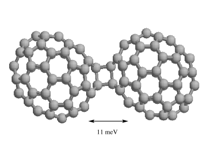
Figure 4: $C_{140}$ with stretch mode shown schematically

The second molecule studied was based on our interest in $C_{140}$. We wanted a molecule with similar properties as $C_{140}$, but with fewer atoms ($C_{72}$). The aim was to increase the accuracy of the basis set used for calculations which would be computationally costly with larger molecules.

Like $C_{140}$, the dominant mode indicated in our calculations was the inter-cage stretch mode which has an energy of 19 meV in $C_{72}$. The molecule is depicted in figure (1). Figures (4) and (1) were produced using Gaussian2003 to minimize the geometry of the molecule and RASMOL to plot out the atom positions.

For both molecules, the low energy modes correspond to large scale motion of the molecules such as the bending, twisting, or stretching of the two cages with respect to each other (acoustic type vibrations) while higher energy modes correspond to motion of the atoms on a smaller scale (optical type vibrations). For example the 15meV mode corresponds to a see-saw motion of the two cages with respect to each other, the 17meV mode corresponds to a twisting motion of the two cages away from a central point, while the higher energy 78 meV mode corresponds to simultaneous deformation of the cages themselves. The vibrations Gaussian calculate are within $5\%$ of the experimental values.

VI Basic Quantities

The shift in the geometrically minimized structure of the $C_{140}$ molecule as it acquires an extra electron (charge) is the predominant factor in determining the amount of phonon emission. If the structure changes little, the overlap between the two ground vibrational states of the initial and final charge state of the molecule will be larger, which suppresses phonon emission since the overlap is a mathematical statement of how likely it is for the molecule to remain in the ground vibrational state rather than transitioning to a excited vibrational state.

It is not known what the natural charge states of our molecule are on a gold substrate, as used in the experiments we compare to. A single $C_{60}$ molecule typically has charge $-2e$ on gold; doubling this, we anticipate that the case of interest may involve a transition from perhaps four to five extra electrons on our molecule.

Table 1 is a chart of the change in the inter-cage distance between the two centers of masses of the fullerene cages upon adding an electron. As one can see, the distance increment increases as the charges increases.

Table 1: Change in distances ($\Delta{\bf{r}}$) between centers of mass of the fullerene cages for $C_{140}$ during different charge transitions ($Q_{1}\rightarrow Q_{2}$) where $Q_{1}$ is the initial charge state of the molecule and $Q_{2}$ is the final charge state of the molecule. Shown are the results of our DFT simulations, and those of our simple model (section VIII).

Transition $Q_{1}\to Q_{2}$	DFT $\Delta{\bf{r}}$ [pm]	Simple $\Delta{\bf{r}}=x[Q_{2}]-x[Q_{1}]$
0 $\rightarrow$ 1	1.005	3.16
1 $\rightarrow$ 2	1.794	9.26
2 $\rightarrow$ 3	2.333	14.8
3 $\rightarrow$ 4	3.056	19.5
4 $\rightarrow$ 5	3.7337	23.4

Therefore, as the charge on the molecule increases, the molecular incremental distortion $\Delta{\bf{r}}$ increases, and consequently the probability that the molecule will remain in the ground vibrational state after an electron has hopped on decreases, leading to stronger phonon sidebands in the differential conductance graphs. Table 2 gives for each electronic transition of the molecule up to a charge state of 5 extra electrons, the total g-factors (equation (39)) in the absence of an applied field, the g-factor associated with the first excited state (eqn 50) where an inter-cage stretch mode phonon is emitted, the probability of the molecule remaining in the ground state ($|O_{0,0}|^{2}$), and the probability that the molecule’s final vibrational state is the first excited state of the stretch mode ($|O_{0,1\alpha=stretch}|^{2}$).

Table 2: $C_{72}$ undergoing different transitions. For convenience we include columns 4 and 5; their result can be deduced from the second and third columns

Table: Probabilities and g-factors for different transitions
Transition	G	$g_{\alpha=stretch}$	$|O_{0,0}|^{2}$	$|O_{0,1\alpha=stretch}|^{2}$
0 $\rightarrow$ 1	0.960	$0.33$	0.38	0.125
1 $\rightarrow$ 2	1.18	$0.406$	0.31	0.126
2 $\rightarrow$ 3	1.27	0.455	0.28	0.127
3 $\rightarrow$ 4	1.29	0.492	0.27	0.135

Figure 5: $g_{\alpha}$ for the $C_{72}$ $0\to 1$ charge-state transition. The large peak is the stretch mode $\alpha=10$ at $19$ meV. Including the two-state emission lines would add an additional peak at $38$ meV (twice the stretch mode) and an otherwise roughly continuous background (see Fig. (10).

Plotting a graph of the $g_{\alpha}$ factor for the electronic transition of a neutral molecule to 1- molecule vs. all 216 modes (as in figure (5)) confirms that the stretch mode of the molecule dominates the single phonon emission. We also plot the corresponding graph of $g_{\alpha}$ for $C_{140}$ in figure (6). As the charge state increases, the effects and phonon sideband strengths will increase. Two phonon emission into separate modes is given by the product of their respective single mode emission while two phonon emission into the same mode is given by equation (96). In any case, the approximation we made for equation (100) suggests that one phonon emission line given by $g_{11meV}$ dominates.

Figure 6: $g_{\alpha}$ for the $C_{140}$ $0\to 1$ charge-state transition. The large peak is the $\alpha=10$ stretch mode at $11$ meV. Again, we estimate that the only significant two-phonon line is at $22$ meV.

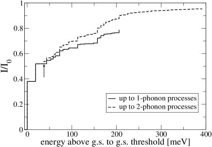
Figure 10: I-V curve predicted for $C_{72}$ for one-phonon process (solid line) and up to two-phonon processes (approximate, dashed line), using the DFT STO-3G basis set. The arrow indicates the position of the two-phonon contribution from the stretch mode.

Again, it is the stretch mode (whose identity is confirmed by displacing the equilibrium coordinates of the molecule by a distortion that is proportional to the eigenmode) that is important. Two-phonon emission may also be significant since experimentally pasupathy1 there is sometimes a second smaller peak at 22meV which may be due to two-phonon emission into the same 11meV mode. Two-phonon emission, however, yields a small contribution to the conductance. For two phonons emitted into the same mode, the contribution is given by the product of the single phonon overlaps. For two phonons emitted into different modes, the contribution cannot be simply described by such a product and the complete expression obtained from integrating the product of the relevant multidimensional gaussians is needed. Although we can calculate the probability of transition to 2-phonon up to n-phonon vibrational final states, we confine ourselves to one-phonon emission in our calculations because as will be illustrated in figure (10) two-phonon emission contributes a continuous background with the only sizeable contribution from two phonon emission into the 11meV mode.

VII Considering External Electric Fields

In reality, the molecule is not in a vacuum but in a real environment of leads and substrate. In the experiments pasupathy1 ; park2 , there is a range of g-factors for different experiments involving the same molecule. This implies that environmental effects play an important role and motivates our calculation of g-factors in the presence of external fields. We account for one feature of this variable environment by applying an electric field to the system. This external field can come about as a result of image charges that are set up across the substrate or across the leads when extra electrons are added to the quantum molecular dot.

In the Gaussian2003 program, we can impose an external field, relax the electronic wavefunction due to the induced polarization and measure the force (expressed as a $3N$ vector, in this case 216-vector) on each atom. The external field will polarize the charge on the molecule as seen in the following representation in figure (7) of the highest occupied molecular orbital under the influence of an external field along the inter-cage bond of the molecule (rendered using the freeware Molden).

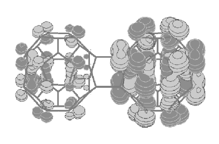
Figure 7: $|\Psi|^{2}$ of the HOMO level of $C_{72}$ under an electric field of $4\times 10^{9}$ V/m along inter-cage bond, showing the polarization of the electron density

This force will then act to distort the molecule’s atomic configuration via lattice relaxation, leading to an increase in pathways available to the electron via vibration assisted tunneling. The initial and final configurations in equations (2),(3),and (6) are ${\bf{r}}_{1}={\bf{r}}_{1}^{(0)}+\mathsf{K}_{1}^{-1}{\bf{f}}_{1}$ and ${\bf{r}}_{2}={\bf{r}}_{2}^{(0)}+\mathsf{K}_{2}^{-1}{\bf{f}}_{2}$, allowing us to calculate the $g_{\alpha}$ factors and hence the phonon emission rates from equation (50). Figure (8) shows that $g_{\alpha}$ for the 11meV line for $C_{140}$ increases substantially under an external field.

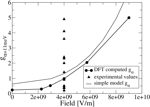
Figure 8: Field dependence of $g_{\alpha}$ for the C₁₄₀ $11$ meV stretch mode from the DFT calculation. The solid line is the field dependence for our simple model calculation which is explained further in section VIII. Experimental values (triangles) are taken at zero field, but included on the plot in a vertical column for visibility

As can be seen in the plot, the field does increase the g-factor from its bare value. At reasonable fields (those that we might expect to find in the experimental literature) such as the region where the field $\approx 3\times 10^{9}V/m$, $g_{\alpha}$ for the most represented mode (the stretch mode) increases to about 0.5. This field would correspond to a charge placed 7 angstroms away. And for a field corresponding to a charge placed 6 angstroms away (the closest plausible distance), $g_{\alpha}$ becomes around 1.0. However, in experiments, the g-factor varies from values of much less than 1 to values as high as 6. In order to reach these quantities in our present theory, we would need to impose much higher and unphysical fields.

Another dependence we examined was the g-factor dependence of the various modes on the angle of a fixed electric field. In figure (9), the electric field was fixed at a value of $4\times 10^{9}$ V/m. The leftmost figure is the 11meV mode – the stretch mode. Following it from left to right are the 3.7 meV mode magnified by a factor of 20,000; the 2.37 meV mode magnified by a factor of 20; the 15 meV mode magnified by a factor of 5; the 17 meV mode magnified by a factor of 200 and finally the 27.6 meV mode magnified by a factor of 500.

The molecule is oriented such that its long axis is aligned vertically. From the figure, we see that there is no coupling of the stretch mode (left shape) to the field when the field is aligned in a direction perpendicular to the stretch mode, and that there is maximum coupling in the direction parallel to the direction of the stretch mode. Note also that $g_{\alpha}$ is non-zero for $\alpha=$stretch mode even in the absence of a field. The symmetries of the plots in figure (9) reflects the symmetry of the modes and how they relate to the symmetry of the applied field. $C_{140}$ has $C_{2h}$ symmetry so it can be generated by a rotation of angle $\pi$ around a fixed axis and a symmetry on a plane orthogonal to the fixed axis. The normal modes of a molecule also possess a definite symmetry with respect to the planes of symmetry of the molecule. The symmetry of the stretch mode is even under reflection in the x-y plane, coinciding with the symmetry of the field $E_{x}$ and orthogonal to the field $E_{z}$. Thus, the strongest coupling of the stretch mode is to $E_{x}$.

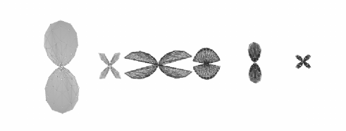
Figure 9: Angle Dependence of $g_{\alpha}=stretch$ for $C_{140}$. Leftmost figure is $g$ plotted as function of the angle of electric field (an extremely high field magnitude of $5\times 10^{12}V/m$) for the 11meV stretch mode; remaining figures to the right are for other modes, and have been magnified considerably to show their shape. The vertical represents fields along the long axis of the molecule.

VIII A simple model for overlaps and fields

To what extent are these quantum overlaps a result of complex quantum chemistry (bonding and anti-bonding and electronic rearrangements inside the two cages)? How much can we understand from simple electrostatics of dumbbells? By modeling the system simply as two rigid balls connected by a spring subject to an external field, we can obtain some understanding at how the dimensions of the problem as well as simple quantities might affect the overlap and g-factor.

We write down the total energy of the system and then minimize the energy with respect to the parameters of our problem and in the presence of an external field – for our case we choose to minimize the charge on one ball and the distance $x$ between the two balls.

The quantities we take into account are as follows:

$$E_{spring} = {1\over{2}}K(x_{2}-x_{1}-a)^{2}$$ (51)

$$E_{field} = q_{1}Ex_{1}+q_{2}Ex_{2}$$ (52)

$$E_{coulomb} = {Kq_{1}q_{2}\over{(x_{2}-x_{1})}}$$ (53)

$$E_{capacitance} = {{1\over{2}}{kq_{1}^{2}\over{r}}}+{{1\over{2}}{kq_{2}^{2}\over{r}}}$$ (54)

where $a$ is the equilibrium distance of the spring, $x_{1}$ and $x_{2}$ are the coordinates of the two balls, $r$ is their radius, $K$ is the spring constant of the system, and $k$ is the Coulomb constant.

We also note that $M_{total}=M_{ball_{1}}+M_{ball_{2}}=2M_{ball}$ and $M_{red}={{M_{ball_{1}}M_{ball_{2}}}\over{M_{ball_{1}}+M_{ball_{2}}}}=M_{ball}/2$ are the well-known center of mass and reduced mass for the system. The last assignment we make are expressions for the charges on each ball ($q_{1}$ and $q_{2}$) in terms of the charges in the system:

$$q_{1} = {Q\over{2}}+{q\over{2}}$$ (55)

$$q_{2} = {Q\over{2}}-{q\over{2}}$$ (56)

where $Q$ is the total charge of the system and $q$ is the difference between the charges on the two balls. The potential energy U then becomes:

$$U = E_{spring}+E_{field}+E_{coulomb}+E_{capacitance}$$ (57)

$$= {1\over{4r(a+x)}}\Big{\{}-2a^{2}Eqr+K(q^{2}(x-r)+Q^{2}(x+r))$$ (58)

$$+ 2rx(2EQX-Eqx+kx^{2})$$ (59)

$$+ a[K(q^{2}+Q^{2})+2r(2EQX-2Eqx+kx^{2})]\Big{\}}.$$ (60)

Here $x=x_{2}-x_{1}$ is the relative distance between the two balls and $X={x_{1}+x_{2}\over{2}}$ is the center of mass coordinates of the system. We next take the derivative of the potential with respect to $q$ the difference in charges on the two balls and set the resulting expression (${dU\over{dq}}$) equal to zero. Solving this expression for $q$ gives us the minimized distribution of charges on the balls under an external field:

$$q={{Er(a+x)^{2}}\over{K(a-r+x)}}.$$ (61)

Similarly, we take the derivative of the potential energy with respect to the deviation from equilibrium $x$ (${dU\over{dx}}$), set this expression equal to zero, and solve for $x$. We keep terms up to second order in $Q$ and $E$ and get:

$$x[Q]=AE^{2}+BQ^{2}+CE^{2}Q^{2}$$ (62)

where $A$, $B$, and $C$ are given by:

$$A = \left({{2a^{2}-5ar-3r^{2}}\over{4kK(a-r)^{3}}}\right)ra^{2}$$ (63)

$$B = {{K(a^{2}+r^{2}-2ar)}\over{4a^{2}k(a-r)^{2}}}$$ (64)

$$C = \left({{2r-a}\over{8k^{2}(a-r)^{3}}}\right)r.$$ (65)

In table (1), we compare the $\Delta r=x[Q_{2}]-x[Q_{1}]$ in the absence of a field for our the simple model and the full DFT calculation discussed earlier where $Q_{1}$ is the total charge for the initial system and $Q_{2}$ is the total charge for the final system. The simple model has between three and six times the distortion of the quantum chemistry calculation, likely due to a combination of more effective screening of the Coulomb repulsion between cages and quantum chemistry effects.

The constants from equation 63 which define the expression for $x$ in equation (62), in combination with the formula for the zero-point motion $x_{0}=\sqrt{{\hbar\over{M_{red}\omega_{0}}}}$ and the one-dimensional equivalent of equation (50) gives us an expression for $G$:

$$g=G={(x[Q_{2}]-x[Q_{1}])^{2}\over{4x_{0}^{2}}}$$ (66)

where in this one-mode limit the log $G$ of the total overlap equals the one-phonon emission ratio $g$. Here $M_{red}$ is is equal to ${70m_{Carbon}\over{2}}$, $\omega_{0}=\omega_{stretch}=11meV$ and the zero-point motion $x_{0}$ for $C_{140}$ is $2.17$ pm.

Therefore, using these formulas our $g$ factor for the $0\to 1$ transition of $C_{140}$ is 0.535 (and for $C_{72}$ it is 0.92). The complete $3N$-dimensional calculations in the absence of a field for the same transition yields a $g_{\alpha}$ for the stretch mode of $0.23$ for $C_{140}$ (and 0.33 for $C_{72}$). This difference is not as large as one would expect from the difference in the center–of–mass motions: the 11meV stretch mode incorporates motions that do not simply change the center of mass separation. In total, the many-body DFT calculations show a stretch–mode phonon emission about a factor of three smaller than that predicted from the simple physical model, and captures the cage size-dependence of $g$, rather well.

Finally, we compare the field dependence of the $g_{\alpha}$ between the simple model and the DFT calculation given in figure (8). The field dependence works out quite well. This simple model could be made more realistic by incorporating features from the DFT calculation (such as charging energies), but that would take us beyond our current illustrative goal.

IX Current due to phonon transitions

Using the g-factors corresponding to all of the different single phonon modes, we graphed a current vs. voltage graph for $C_{72}$ using the simplified formula where all the phonons are identical in both charge states of the molecule. Figure (11) gives the current divided by $I_{0}$ vs. the available energy above the ground state to ground state threshold for both one-phonon emission processes (solid line) and up to two-phonon processes (dashed line). The plots are constructed by iteratively calculating phonon emission from a pool of available energy. As energy decreases, less is available for emitting phonons. Our $g_{\alpha}$’s make use of the fact that the phonon quadratic forms $\Omega$ change between different charge states.

As you can see, the currents due to one-phonon processes and for up to two phonon processes share similar gross features at the beginning such as the jump in current at the $19$ meV energy mode corresponding to the stretch mode of the molecule. However they start to deviate as energy increases until they level off at different values of current (0.8 for the one-phonon process and 0.95 for the two-phonon processes) which would seem to indicate that two-phonon processes will play a role in the I-V characteristics of a molecular quantum dot.

In addition, the I-V curve that includes all n-phonon processes will asymptote to one. The two-phonon contribution forms almost a continuous background, except for $2\omega_{stretch}$, whose position is shown with an arrow in figure (11). We also note that the our treatment of two-identical-phonon emission is (for convenience) not the correct formula derived in equation (96) which allows the frequencies to change between the initial and final states, but the approximate formulas given by equations 67 and 68.

$$O_{0,2\alpha}\approx e^{-G}g_{\alpha}^{2}/2$$ (67)

$$I/I_{0}(E) = \sum_{\alpha}(0_{0,1\alpha}\Theta(E-\hbar\omega_{alpha})+O_{0,2\alpha}\Theta(E-2\hbar\omega_{\alpha}))$$ (68)

$$+ \sum_{\alpha,\alpha^{\prime}\neq\alpha}O_{0,1\alpha 1\alpha^{\prime}}\Theta(E-\hbar\omega_{\alpha}-\hbar\omega_{\alpha^{\prime}})$$ (69)

As one may observe, the approximate two-phonon rates form a featureless background except for the 2-stretch-mode phonon peak, a result of the weak couplings to the other modes.

X Conclusion

There is much recent interest in vibrating mechanical systems coupled to electron transport on the nanoscale, from nanomechanical resonators LaHaye ; Naik to single-electron shuttles Gorelik ; Blick . Vibrational effects on electron transport through molecules have been studied since the 1960s in devices containing many molecules Jaklevic , and more recently have been shown to be important in transport through single molecules measured using scanning tunneling microscopes stipe , single-molecule transistors park1 ; park2 ,and mechanical break junctions smit . In a natural extension of work done in the 1920s by Franck, Condon, et al. in atomic spectra, we have studied the effects of molecular vibrations on electron transport through a molecule. We have shown that density functional theory calculations of the normal modes and deformations, coupled to a straightforward linear algebra calculation, can provide quantitative predictions for the entire differential tunneling spectrum, even including external fields from the molecular environment.

X.1 Acknowledgments

We would like to thank Jonas Goldsmith and Geoff Hutchinson for helpful conversations. We would also like to thank the two referees for their careful reading of the manuscript and their many helpful suggestions for improvement. We acknowledge support from NSF grants DMR-0218475 and CHE-0403806 and from a GAANN fellowship DOEd P200A030111.

XI Appendix

Here we show how one can calculate the Franck-Condon factor for a transition from the neutral ground state to an excited state with one vibrational mode in a doubly-excited state. (For emission into general excited states, we would need to use the appropriate multi-dimensional gaussian multiplied by the appropriate Hermite polynomials. This calculation quickly becomes complicated KRLC93 , and for the molecules of interest to us, multiple phonon emission is rare.) From the vibrational states given in (20), we’re interested in the following integral:

$$O_{0,2}=\int\,d{\bf{y}}{\Psi_{0}^{(1)*}({\bf{y}})\Psi_{2,\alpha}^{(2)}({\bf{y}}-{\bf{\Delta}})}$$ (70)

where we can split the integral into two parts:

$$=\int\,d{\bf{y}}N_{1}N_{2}\sqrt{2}\omega_{\alpha}[{{\mbox{\boldmath$\epsilon$}}}_{\alpha}^{(2)}\cdot{({\bf{y}}-{\bf{\Delta}})}]^{2}e^{-{1\over{2\hbar}}\left({\bf{y}}^{\dagger}\mathsf{\Omega}_{1}{\bf{y}}\right)}$$ (71)

$$\times e^{-{1\over{2\hbar}}\left(({\bf{y}}-{\bf{\Delta}})^{\dagger}\mathsf{\Omega}_{2}({\bf{y}}-{\bf{\Delta}})\right)}$$ (72)

$$-\int\,d{\bf{y}}N_{1}N_{2}\sqrt{2}{1\over{2}}e^{-{1\over{2\hbar}}\left({\bf{y}}^{\dagger}\mathsf{\Omega}_{1}{\bf{y}}\right)}e^{-{1\over{2\hbar}}\left({\bf{y}}-{\bf{\Delta}})^{\dagger}\mathsf{\Omega}_{2}({\bf{y}}-{\bf{\Delta}})\right)}.$$ (73)

Expression (73) is just $-{1\over{\sqrt{2}}}O_{0,0}$; we concentrate on expression (71). First, as we did for the $O_{0,1}$ case, we rewrite this integral in terms of the quantities $\tilde{{\bf{\Delta}}}$ and $\mathsf{\bar{\Omega}}$:

$$N_{1}N_{2}\sqrt{2}({\omega_{\alpha}\over{\hbar}})\int{d{\bf{y}}}[\hat{{{\mbox{\boldmath$\epsilon$}}}}_{\alpha}^{(2)}\cdot({\bf{y}}-{\bf{\Delta}})]^{2}e^{-{1\over{\hbar}}({\bf{y}}-\tilde{{\bf{\Delta}}})^{\dagger}\mathsf{\bar{\Omega}}({\bf{y}}-\tilde{{\bf{\Delta}}})}$$ (74)

$$\times e^{-{1\over{2\hbar}}{{\bf{\Delta}}^{\dagger}\mathsf{\Omega}_{2}{\bf{\Delta}}}}e^{{1\over{2\hbar}}{\tilde{{\bf{\Delta}}}(\mathsf{\Omega}_{1}+\mathsf{\Omega}_{2})\tilde{{\bf{\Delta}}}}}.$$ (75)

We want to make this expression look like the known gaussian integral: $C_{1}\int{dx\,x^{2}e^{-x^{2}+C_{2}}}$ where $C_{1}$ and $C_{2}$ are constants. Changing variables to $\tilde{{\bf{y}}}$:

$$\tilde{{\bf{y}}}={\bf{y}}-\tilde{{\bf{\Delta}}}$$ (76)

$$d\tilde{{\bf{y}}}=d{\bf{y}}$$ (77)

$${\bf{y}}=\tilde{{\bf{y}}}+\tilde{{\bf{\Delta}}}$$ (78)

we rewrite the integral as one over $d^{n}\tilde{y}$:

$$N_{1}N_{2}\sqrt{2}({\omega_{\alpha}\over{\hbar}})\int{d\tilde{{\bf{y}}}}[\hat{{{\mbox{\boldmath$\epsilon$}}}}_{\alpha}^{(2)}\cdot(\tilde{{\bf{y}}}+\tilde{{\bf{\Delta}}}-{\bf{\Delta}})]^{2}e^{-{1\over{\hbar}}\tilde{{\bf{y}}}^{\dagger}\mathsf{\bar{\Omega}}\tilde{{\bf{y}}}}$$ (79)

$$\times e^{-{1\over{2\hbar}}{{\bf{\Delta}}^{\dagger}\mathsf{\Omega}_{2}{\bf{\Delta}}}}e^{{1\over{2\hbar}}{\tilde{{\bf{\Delta}}}(\mathsf{\Omega}_{1}+\mathsf{\Omega}_{2})\tilde{{\bf{\Delta}}}}}.$$ (80)

Expanding out the term in brackets in equation (79), we get:

$$[\hat{{{\mbox{\boldmath$\epsilon$}}}}_{\alpha}^{(2)}\cdot\tilde{{\bf{y}}} + \hat{{{\mbox{\boldmath$\epsilon$}}}}_{\alpha}^{(2)}\cdot(\tilde{{\bf{\Delta}}}-{\bf{\Delta}})]^{2}=[\hat{{{\mbox{\boldmath$\epsilon$}}}}_{\alpha}^{(2)}\cdot\tilde{{\bf{y}}}+{\bf{d}}^{2}]^{2}$$ (81)

$$= (\hat{{{\mbox{\boldmath$\epsilon$}}}}_{\alpha}^{(2)}\cdot\tilde{{\bf{y}}})^{2}+2{\bf{d}}(\hat{{{\mbox{\boldmath$\epsilon$}}}}_{\alpha}^{(2)}\cdot\tilde{{\bf{y}}})+{\bf{d}}^{2}$$ (82)

where $d=\hat{{{\mbox{\boldmath$\epsilon$}}}}_{\alpha}^{(2)}\cdot(\tilde{\bf{\Delta}}-{\bf{\Delta}})$.

The second term in equation (81) will be zero in the integral because of symmetry considerations which dictate that odd powered gaussian integrals of the form: $\int\,dx\,x^{n}e^{-x^{2}}$ where $n$ is odd always equal zero.. The only terms in the integral of equation (79) that remain are the first term and the constant ${\bf{d}}^{2}$.

We transform this integral into the appropriate normal mode basis. Since, we are integrating over the coordinates centered on $\tilde{\bf{\Delta}}$ for a system with a Hessian of $\mathsf{\bar{\Omega}}$, we want to rewrite everything in terms of the eigenmodes of the averaged $\mathsf{\bar{\Omega}}$. We’ll call these eigenmodes $\hat{{{\mbox{\boldmath$\rho$}}}}_{\beta}$ where the following definitions hold:

$$\tilde{{\bf{y}}} = \sum_{\beta}p_{\beta}\hat{{{\mbox{\boldmath$\rho$}}}}_{\beta}$$ (83)

$$\mathsf{\bar{\Omega}}\hat{{{\mbox{\boldmath$\rho$}}}}_{\beta} = \bar{\omega}_{\beta}\hat{{{\mbox{\boldmath$\rho$}}}}_{\beta}.$$ (84)

Here, $\hat{{{\mbox{\boldmath$\rho$}}}}_{\beta}$ are the orthonormal eigenvectors for $\mathsf{\bar{\Omega}}$ and $p_{\beta}$ are the weightings of each mode’s contribution to $\tilde{{\bf{y}}}$. Hence:

$$(\hat{\mbox{\boldmath$\epsilon$}}_{\alpha}^{(2)}\cdot\tilde{{\bf{y}}})^{2} = (\sum_{\beta}p_{\beta}\hat{\mbox{\boldmath$\epsilon$}}_{\alpha}^{(2)}\cdot\hat{\mbox{\boldmath$\rho$}}_{\beta})^{2}$$ (85)

$$= \sum_{\beta}p_{\beta}^{2}(\hat{\mbox{\boldmath$\epsilon$}}_{\alpha}^{(2)}\cdot\hat{\mbox{\boldmath$\rho$}}_{\beta})^{2}$$ (87)

$$+\sum_{\beta\neq\beta^{{}^{\prime}}}p_{\beta}p_{\beta^{{}^{\prime}}}(\hat{\mbox{\boldmath$\epsilon$}}_{\alpha}^{(2)}\cdot\hat{\mbox{\boldmath$\rho$}}_{\beta})(\hat{\mbox{\boldmath$\epsilon$}}_{\alpha}^{(2)}\cdot\hat{\mbox{\boldmath$\rho$}}_{\beta^{{}^{\prime}}}).$$

Again, the second term is odd in the new integration variables $p_{\beta}$ and will be zero. Rewriting the integral in $d\vec{p}$ and remembering that $\hat{\rho}$ diagonalizes $\bar{\Omega}$, the integral from equation (70) and (79) becomes:

$$N_{1}N_{2}\sqrt{2}({\omega_{\alpha}\over{\hbar}})[\int{d^{n}p}\sum_{\beta}p_{\beta}^{2}(\hat{\mbox{\boldmath$\epsilon$}}_{\alpha}^{(2)}\cdot\hat{\mbox{\boldmath$\rho$}}_{\beta})^{2}e^{-{1\over{\hbar}}\sum_{\beta^{{}^{\prime}}}p_{\beta^{{}^{\prime}}}^{2}\omega_{\beta^{{}^{\prime}}}}]$$ (89)

$$\times e^{-{1\over{2\hbar}}{{\bf{\Delta}}^{\dagger}\mathsf{\Omega}_{2}{\bf{\Delta}}}}e^{{1\over{2\hbar}}{\tilde{{\bf{\Delta}}}(\mathsf{\Omega}_{1}+\mathsf{\Omega}_{2})\tilde{{\bf{\Delta}}}}}$$

$$= N_{1}N_{2}\sqrt{2}({{\omega_{\alpha}}\over{\hbar}})\sum_{\beta}(\hat{\mbox{\boldmath$\epsilon$}}_{\alpha}^{(2)}\cdot\hat{\mbox{\boldmath$\rho$}}_{\beta})^{2}[\int{d^{n}p}p_{\beta}^{2}e^{-{1\over{\hbar}}\sum_{\beta^{{}^{\prime}}}p_{\beta^{{}^{\prime}}}^{2}\bar{\omega}_{\beta^{{}^{\prime}}}}]$$ (91)

$$\times e^{-{1\over{2\hbar}}{\bf{\Delta}}^{\dagger}\mathsf{\Omega}_{2}{\bf{\Delta}}}e^{{1\over{2\hbar}}{\tilde{{\bf{\Delta}}}(\mathsf{\Omega}_{1}+\mathsf{\Omega}_{2})\tilde{{\bf{\Delta}}}}}.$$

But $\int x^{2}e^{-Ax^{2}}dx={\sqrt{\pi}\over{2A^{3/2}}}={1\over{2A}}\int e^{-Ax^{2}}dx$, so

$$\int{d^{n}p}\,p_{\beta}^{2}\,e^{-{1\over{\hbar}}\sum_{\beta^{{}^{\prime}}}p_{\beta^{{}^{\prime}}}^{2}\bar{\omega}_{\beta^{{}^{\prime}}}} = {1\over{2\bar{\omega}_{\beta}/\hbar}}\sqrt{{{\pi\hbar}\over{\bar{\omega}_{\beta}}}}\prod_{\beta^{{}^{\prime}}\neq\beta}\sqrt{{\pi\hbar}\over{\bar{\omega}_{\beta^{{}^{\prime}}}}}$$ (92)

$$= \frac{\hbar}{2\bar{\omega}_{\beta}}\frac{1}{\bar{N}^{2}}.$$ (93)

Hence, the first term in (81) from equation (89) becomes:

$$N_{1}N_{2}\sqrt{2}({{\omega_{\alpha}}\over{\hbar}})\sum_{\beta}(\hat{\mbox{\boldmath$\epsilon$}}_{\alpha}^{(2)}\cdot\hat{\mbox{\boldmath$\rho$}_{\beta}})^{2}{{\hbar}\over{2\bar{\omega}_{\beta}}}{1\over{\bar{N}^{2}}}e^{{1\over{\hbar}}\tilde{{\bf{\Delta}}}^{\dagger}\mathsf{\bar{\Omega}}\tilde{{\bf{\Delta}}}}e^{-{1\over{2\hbar}}{\bf{\Delta}}^{\dagger}\mathsf{\Omega}_{2}{\bf{\Delta}}}$$ (94)

which from equation (38) we see is

$$O_{0,0}\sqrt{2}\omega_{\alpha}\sum_{\beta}{1\over{2\bar{\omega}_{\beta}}}(\hat{\mbox{\boldmath$\epsilon$}}_{\alpha}^{(2)}\cdot\hat{\mbox{\boldmath$\rho$}}_{\beta})^{2}.$$ (95)

Combining this with the third term from equation (81) and expression (73), our expression for the $0\rightarrow 2$ overlap becomes:

$$O_{0,2_{\alpha}} = O_{0,0}\Big{\{}\sqrt{2}\omega_{\alpha}\sum_{\beta}{1\over{2\bar{\omega}_{\beta}}}(\hat{\mbox{\boldmath$\epsilon$}}_{\alpha}^{(2)}\cdot\hat{\mbox{\boldmath$\rho$}}_{\beta})^{2}$$ (96)

$$+ \sqrt{2}({\omega_{\alpha}\over{\hbar}})[\hat{\mbox{\boldmath$\epsilon$}}_{\alpha}^{(2)}\cdot(\tilde{{\bf{\Delta}}}-{\bf{\Delta}})]^{2}-{1\over{\sqrt{2}}}\Big{\}}$$ (97)

$$= O_{0,0}\Big{\{}\sum_{\beta}{\omega_{\alpha}\over{\sqrt{2}\bar{\omega}_{\beta}}}(\hat{\mbox{\boldmath$\epsilon$}}_{\alpha}^{(2)}\cdot\hat{\mbox{\boldmath$\rho$}_{\beta}})^{2}$$ (98)

$$+ \sqrt{2}({\omega_{\alpha}\over{\hbar}})[\hat{\mbox{\boldmath$\epsilon$}}_{\alpha}^{(2)}\cdot(\tilde{{\bf{\Delta}}}-{\bf{\Delta}})]^{2}-{1\over{\sqrt{2}}}\Big{\}}.$$ (99)

If $\mathsf{\Omega_{1}}=\mathsf{\Omega}_{2}$ (i.e., there is no change in the harmonic potential), $\mathsf{\bar{\Omega}}=\mathsf{\Omega}_{2}$ and hence $\hat{\mbox{\boldmath$\epsilon$}}_{\alpha}^{(2)}\cdot\hat{\mbox{\boldmath$\rho$}}_{\beta}=\delta_{\alpha\beta}$ and $\bar{\omega}_{\beta}=\omega_{\beta}$. The first sum reduces to ${1\over{\sqrt{2}}}$, canceling the last term. Therefore in this case:

$$|{O_{0,2\alpha}\over{O_{0,0}}}|^{2}=2{({\omega_{\alpha}\over{\hbar}})}^{2}[\hat{\mbox{\boldmath$\epsilon$}}_{\alpha}^{(2)}\cdot(\tilde{{\bf{\Delta}}}-{\bf{\Delta}})]^{4}={g_{\alpha}^{2}\over{2}}.$$ (100)

The change in harmonic potential upon charging the molecule allows for phonon emission even in the absence of a configurational shift. Therefore, even if ${\bf{\Delta}}=\tilde{\bf{\Delta}}=0$, phonons can be emitted both because of frequency shifts $(\omega_{\alpha}\neq\bar{\omega}_{\beta})$ and because the normal modes change $(\hat{\mbox{\boldmath$\epsilon$}}_{\alpha}\neq\hat{\mbox{\boldmath$\rho$}}_{\beta})$.

The other overlaps could be performed in a similar way. The strategy is to write everything in terms of integrals of $\int dxx^{n}e^{-x^{2}}$ by transforming to the basis of the averaged gaussian with $\bar{\Omega}$. The odd powered integrals are eliminated and the even powered terms remain.

References

- (1) J.H. Schulman and W.D. Compton. Color Centers in Solids. MacMillan Company, New York, NY, 1962.
- (2) C.P. Flynn and A.M. Stoneham. Phys. Rev. B, 1(10):3966, 1987.
- (3) E.M. Conwell, H.Y. Choi, and S. Jeyadev. J. Phys. Chem., 96:2827, 1992.
- (4) D. Boese and H. Schoeller. Europhys. Lett., 54:668, 2001.
- (5) S Braig and K. Flensberg. Phys. Rev. B, 68:205324, 2003.
- (6) A. Mitra, I. Aleiner, and A.J. Millis. Phys. Rev. B, 69:245302, 2004.
- (7) X.H. Qiu, G.V. Nazin, and W. Ho. Phys. Rev. Lett., 92:206102, 2004.
- (8) B.C. Stipe, M.A. Rezaei, and W. Ho. Science, 280:1732, 1998.
- (9) RHM Smit, Y. Noat, C. Untiedt, N.D. Lang, M.C. van Hemert, and J.M. van Ruitenbeek. Nature, 419:906, 2002.
- (10) H. Park, J. Park, A.K.L. Kim, E.H. Anderson, A.P. Alivisatos, and P.L. McEuen. Nature, 57:407, 2000.
- (11) J. Park, A.N. Pasupathy, J.I. Goldsmith, C. Chang, Y. Yaish, J.R. Petta, M. Rinkoski, J.P. Sethna, H.D. Abruna, P.L. McEuen, and D.C. Ralph. Nature, 417:722, 2002.
- (12) J. Koch and F. von Oppen. Phys. Rev. B, 72:113308, 2005.
- (13) M.R. Wegewijs and K.C. Nowack. New J. of Phys., 7:239, 2005.
- (14) A. Nitzan. Ann. Rev. Phys. Chem., 52:681, 2001.
- (15) F. Duschinsky. Acta Physicochim. URSS, 7:551, 1937.
- (16) D.W. Kohn, E.S.J. Robles, C.F. Logan, and P. Chen. J. Phys. Chem., 97:4936, 1993.
- (17) F. Chau, J.M. Dyke, E. P. Lee, and D. Wang. J. of Electron Spectroscopy and Related Phenomena, 97:33, 1998.
- (18) G.C. Schatz and M.A. Ratner. Quantum Mechanics in Chemistry. Prentice Hall, Englewood Cliffs, NJ, 1993.
- (19) G. Herzberg. Molecular Spectra and Molecular Structure: I. Spectra of Diatomic Molecules. Van Nostrand Reinhold, NY, NY, 1950.
- (20) Coon J.B., Dewames R.E., and C.M. Loyd. J. Mol. Spectrosc., 8:285, 1962.
- (21) J. Franck. Faraday Soc., 21:536, 1925.
- (22) E.U. Condon. Phys. Rev., 32:858, 1928.
- (23) B.J. LeRoy, S.G. Lemay, J. Kong, and C. Dekker. Nature, 432:371–374. 2004.
- (24) M. Butticker, Y. Imry, R. Landauer and S. Pinhas. Phys. Rev. B, 31:6207–6215, 1985.
- (25) C.W.J. Beenakkr and H. van Houten. Solid State Physics: Semiconductor Heterostructures and Nanostructures.
- (26) R. Landauer. IBM J. Res. Dev., 1:233, 1957.
- (27) C.W.J. Beenakker. Phys. Rev. B, 44:1646–1656, 1991.
- (28) L.I. Glazman and R.I.Shekhter. Sov. Phys. JETP, 67:163, 1988.
- (29) A.N. Pasupathy, J. Park, C. Chang, A.V. Soldatov, S. Lebedkin, R.C. Bialczak, J.E. Grose, L.A.K. Donev, J.P. Sethna, D.C. Ralph, and P.L. McEuen. Nano Lett., 5(2):203, 2005.
- (30) S. Lebedkin, W.E. Hull, A. Soldatov, B. Renker, and M.M. Kappes. J. Phys. Chem. B., 104:4101, 2000.
- (31) MD LaHaye, P. Buu, B. Camarota, and KC Schwab. Science, 304:74, 2004
- (32) A. Naik, O. Buu1, MD LaHaye, AD Armour, AA Clerk, MP Blencowe and KC Schwab. Nature, 443:193, 2006
- (33) LY Gorelik, A. Isacsson, MV Vonova, B Kasemo, RI Shekhter and M. Jonson. Phys. Rev. Lett., 80:4526, 1998
- (34) A. Erbe, Blick RH, A. Tilke, A. Kriele and JP Kotthaus. Appl. Phys. Lett., 73:3751, 1998
- (35) RC Jaklevic and J. Lambe. Phys. Rev. Lett., 17:1139, 1966