Nonuniform Self-Organized Dynamical States in Superconductors with Periodic Pinning

Abstract

We consider magnetic flux moving in superconductors with periodic pinning arrays. We show that sample heating by moving vortices produces negative differential resistivity (NDR) of both N and S type (i.e., N- and S-shaped) in the voltage-current characteristic (VI curve). The uniform flux flow state is unstable in the NDR region of the VI curve. Domain structures appear during the NDR part of the VI curve of an $N$ type, while a filamentary instability is observed for the NDR of an $S$ type. The simultaneous existence of the NDR of both types gives rise to the appearance of striking self-organized (both stationary and non-stationary) two-dimensional dynamical structures.

Semiconductor devices sch exhibiting Negative Differential Resistivity (NDR) and Conductivity (NDC) have played a very important role in science and technology. These useful devices include sch : Gunn effect diodes, $pnpn$-junctions, etc. Here we study superconducting analogs of these semiconductor devices. Table 1 briefly compares NDR in superconductors, semiconductors, plasmas, and manganites. Conceptually, the non-uniform self-organized structures (e.g., filaments and overheated domains with higher or lower electric fields) are related for superconductors, plasmas, and semiconductors. However, the physical mechanism giving rise to the instability of the homogeneous state can be different in each case.

The magnetic flux behavior in superconductors with artificial pinning sites has attracted considerable attention due to the possibility of constructing samples with desired properties vvmdotprl ; fnsc2003 ; rwdot ; vvmbdot ; vvmfddot . Among such systems, samples with Periodic Arrays of Pinning Sites (PAPS) are studied intensely because advanced fabrication techniques allow to design well-defined periodic structures with controlled microscopic pinning parameters. For such systems, Ref. fn1, has revealed the existence of several dynamical vortex phases, which are similar to the ones shown in the inset of Fig. 1. At low current density $j$, the vortices are pinned and their average velocity, $\bar{v}$, is zero (phase I). Here $\bar{v}=N_{v}^{-1}\sum_{i}\mathbf{v}_{i}\cdot\mathbf{x}$, is the average vortex velocity in the $x$ direction. At higher $j,$ interstitial vortices start to move and the flux velocity increases with the drive (phase II). Then, a sharp jump in $\bar{v}(j)$ occurs since a fraction of the vortices depins and a very disordered uniform phase arises (phase III). This phase is analogous to the uniform electron motion in semiconductor devices. After increasing the applied current $j$ (for superconductors) or the applied voltage (for semiconductors), the vortex (electron) velocity shows a remarkable and non-intuitive sudden drop (i.e., the velocity drops even though the applied force increases). Indeed, when $j$ exceeds a threshold value, only incommensurate vortex rows move (phase IV). Finally, the increasing driving force completely overcomes the pinning (phase V). The dependence $\bar{v}(j)$ describes the voltage-current characteristic (VI curve) since the electric field $E$ is related to $\bar{v}$ by $E=-\bar{v}(j)B/c$. Here we prove that the flux motion in samples with PAPS results in an unusual, for superconductors, VI curve with NDR of the so-called $S$ type sch ; kun . That is, within some interval of voltages there exist three different current values corresponding to a single electric field. Such types of $S$-shaped VI curves play a very important role in plasmas and semiconductors, and give rise to a filamentary instability when a uniform current flow breaks into filaments with lower and higher current densities sch .

	Superconductors	Semiconductors	Plasmas	Manganites
Carriers	flux quanta	charge quanta:	electrons	electrons,
		electrons or holes		holes
Characteristic curve	voltage-current	current-voltage	IV curve	IV curve
	(VI) curve	(IV) curve
Homogeneous state	homogeneous flux	homogeneous	homogeneous	homogeneous
	and current flows	current flow	current flow	current flow
Origin of S-shape	in/commensurate vortex	non-linear electron	ionization	$-$
NDR	dynamical phases in PAPS	transport
Origin of N-shape	overheating, Cooper pair	overheating, electron	heating cap	heating tokunaga2
NDR	tunnelling Hueb ; vortex-core:	or hole tunnelling
	shrinkage LO ($T\approx T_{c}$);
	expansion kun , driven doettinger ($T\ll T_{c}$)
Filaments	supercurrent filaments	normal current filaments	pinch-effect	$-$
Domains	vortex-induced higher $E$	higher $E$	higher $E$	higher $E$
	field overheated domains	overheated domains	overheated domains	overheated domains

Table 1: Comparison between non-uniform non-equilibrium states in superconductors, semiconductors, plasmas, and manganites with VI curves having Negative Differential Resistivity (NDR). Since $IV$ curves in semiconductors map to $VI$ curves in superconductors, then NDC (for semiconductors) maps into NDR for superconductors. Here, $N$($S$) type shapes for semiconductors correspond to $S$($N$) type for superconductors GMR . The Negative Differential Conductivity (NDC) found in kun is analogous to the Gunn effect in semiconductors, where electron-charge modulations lead to steps in $j(E)$ in the NDC regime.

Sufficiently strong disorder in the pinning array gives rise to the disappearance of the described dynamical phase transitions fn1 and, consequently, the vanishing of the NDR for $S$-shaped VI curves. Higher thermal fluctuations also result in such an effect. Experimentally, the current density, $j$, at which the flux flow regime is observed in superconductors, is usually high BL ; GMR , and the Joule heat should also affect the picture described above. An increase in temperature $T$ results in a decrease of the pinning force. Thus, the current density can decay with increasing electric field, and a $N$-shaped VI curve with a NDR of $N$ type (red dashed line in Fig. 1) is commonly observed in superconductors for high current density GMR ; GM . The uniform state in samples with NDR of $N$ type is also unstable sch ; and a propagating resistive state boundary or the formation of resistive domains can destroy the uniform superconducting state GMR ; GM ; Hueb . For certain pinning parameters and cooling conditions, one can achieve a situation where the NDR of both $N$ and $S$ type simultaneously coexist in the VI curve (Fig. 1). In this case, we predict remarkable flux flow instabilities.

Here, we study the effect of Joule heating and disorder on the VI curve of superconductors with PAPS. Based on analytical and numerical analysis of the VI curve, we find the conditions under which the VI curve has a NDR region of either $S$ type or $N$ type, or both. We discuss the effect of the shape of the NDR on the vortex and current flow. We argue that the coexistence of the NDR of both, $S$ and $N$ types, gives rise to the macroscopically non-uniform self-organized dynamical structures in the flux flow regime.

We numerically integrate the two-dimensional overdamped equations of motion fn1 ; md01 ; md03Z for the flux lines driven, by the current $j$, in the $x$ direction over a square PAPS with lattice constant $a$: $\eta\mathbf{v}_{i}=\mathbf{F}_{i}^{vv}+\mathbf{F}_{i}^{vp}+\mathbf{F}_{i}^{T}+\mathbf{F}_{d}.$ Here $\eta$ is the flux flow viscosity BL , $\mathbf{v}_{i}$ is the velocity of $i$th vortex, $\mathbf{F}_{i}^{vv}$ is the force acting on the $i$th vortex per unit length due to the interaction with other vortices, $\mathbf{F}_{i}^{vp}$ is the $i$th vortex-pin interaction, $F_{d}=j\phi_{0}/c$ is the driving force, and $\phi_{0}$ is the flux quantum. The thermal fluctuation contribution to the force, $\mathbf{F}_{i}^{T}$, satisfies: $\langle F_{i}^{T}(t)\rangle_{t}=0$ and $\langle F_{i}^{T}(t)F_{j}^{T}(t^{\prime})\rangle_{t}=2\eta k_{B}T\delta_{ij}\delta(t-t^{\prime})$.

The vortex-vortex interaction is modelled by $\mathbf{F}_{i}^{vv}=\left(\phi_{0}^{2}/8\pi^{2}\lambda^{3}(T)\right)\sum_{j=1}^{N_{v}}K_{1}\left(|\mathbf{r}_{i}-\mathbf{r}_{j}|/\lambda(T)\right)\mathbf{\widehat{r}}_{ij},$ $K_{1}$ is the modified Bessel function, the summation is performed over the positions $\mathbf{r}_{j}$ of $N_{v}$ vortices in the sample, and $\mathbf{\widehat{r}}_{ij}=(\mathbf{r}_{i}-\mathbf{r}_{j})/|\mathbf{r}_{i}-\mathbf{r}_{j}|$. The temperature dependence of the penetration depth $\lambda$ is approximated as $\lambda(T)=\lambda_{0}(1-T^{2}/T_{c}^{2})^{-1/2}$. The Ginzburg-Landau formula for $H_{c2}(T)$ is used and we assume that the ratio $\kappa_{GL}=\lambda/\xi$ is temperature independent (here $\xi$ is the coherence length). The pinning is modelled as $N_{p}$ parabolic wells located at positions $\mathbf{r}_{k}^{(p)}$. The pinning force per unit length is $\mathbf{F}_{i}^{vp}=\left(F_{p}(T)/r_{p}\right)\sum_{k=1}^{N_{p}}|\mathbf{r}_{i}-\mathbf{r}_{k}^{(p)}|\Theta\left(r_{p}-|\mathbf{r}_{i}-\mathbf{r}_{k}^{(p)}|/\lambda_{0}\right)\mathbf{\widehat{r}}_{ik}^{(p)},$ where $r_{p}$ is the range of the pinning potential, $\Theta$ is the Heaviside step function, and $\mathbf{\widehat{r}}_{ik}^{(p)}=(\mathbf{r}_{i}-\mathbf{r}_{k}^{(p)})/|\mathbf{r}_{i}-\mathbf{r}_{k}^{(p)}|$. We estimate the maximum pinning force, $F_{p}=F_{p}(T)$, as $H_{c}^{2}\xi^{2}/r_{p}$ and, thus, $F_{p}(T)=F_{p0}(1-T^{2}/T_{c}^{2})$.

For brevity, the simulations shown here are for $18\times 12$ $\lambda_{0}^{2}$ periodic cells and at magnetic fields near the first matching field, $B_{\phi}=\phi_{0}/a^{2}$, where $N_{p}=N_{v}$. First, we start with a high-temperature vortex liquid. Then, the temperature is slowly decreased down to $T=0$. When cooling down, vortices adjust themselves to minimize their energy, simulating field-cooled experiments. Then we increase the driving current and compute the average vortex velocity $\bar{v}(j)$.

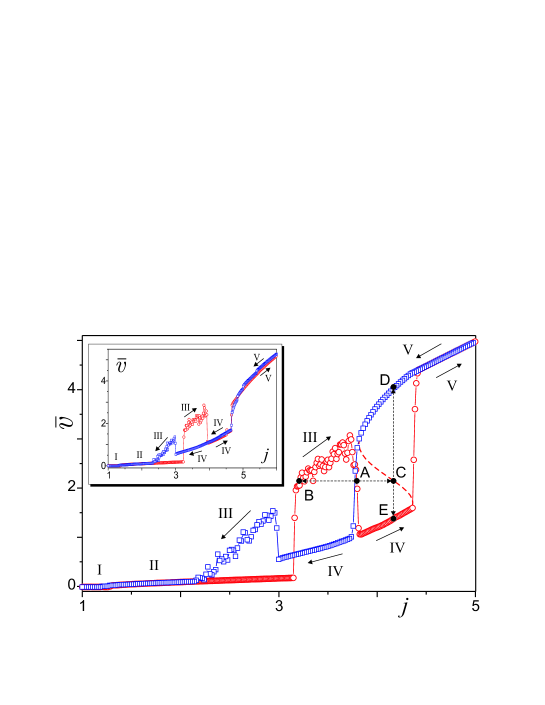
Figure 1: (Color online) The average vortex velocity $\bar{v}\propto E$ vs current $j$ for $B/B_{\Phi}=1.074$, $r_{p}=0.2\lambda_{0}$ and $F_{p}/F_{0}=2$ for increasing (red open circles) and for decreasing (blue open squares) $j$. State A is unstable and the sample divides into filaments, some in states B and some in C. State C is also unstable. The corresponding stable states are on the lower (point E) and on the upper (point D) VI curve branches. Inset: VI curve when no heating effects are taken into account.

The average power of Joule heating per unit volume is $jE=j\bar{v}B/c$. We assume that the temperature relaxation length is larger than any local scale and the sample thickness. Under such conditions, the local temperature increase due to vortex motion can be found from the heat balance equation GMR : $h_{0}S\left(T-T_{0}\right)=\bar{v}jBV/c$, where $h_{0}$ is the heat transfer coefficient, $T_{0}$ the ambient temperature, and $S$ and $V$ are the sample surface and volume. Further, we shall assume that $T_{0}\ll T_{c}$ and neglect $T_{0}$. We define the dimensionless driving force as $f_{d}=j/j_{0}$ and introduce the dimensionless parameters $V_{x}=\bar{v}/v_{0}$ and $b=B/B_{\phi}$, where $v_{0}=c^{2}/4\pi\kappa^{2}_{GL}\sigma_{n}\lambda_{0}$, and $j_{0}=c\phi_{0}/8\pi^{2}\lambda_{0}^{3}$. We assume that the normal state conductivity $\sigma_{n}$ is temperature-independent. As a result, the temperature and the driving force are related by: $T/T_{c}=K_{th}\,V_{x}\,f_{d}\,b$, where $K_{th}=j_{0}\,v_{0}\,B_{\phi}\,V/c\,h_{0}\,T_{c}\,S$ is the ratio of the characteristic heat release to heat removal. Using the rough estimates $\lambda_{0}=2000$ Å, $\kappa_{GL}=100$, $\sigma_{n}=10^{16}$ s^-1, $V/S=1000$ Å, $T_{c}=90$ K, $B_{\phi}=500$ G, and $h_{0}=1$ W/cm²K, we find $K_{th}=0.05-0.06$ and $F_{p0}$ is of the order of $F_{0}=\phi_{0}j_{0}/c$. In the simulations, we used $K_{th}=0.0525$.

The velocity $\bar{v}$ versus current $j$ (which coincides with the sample VI curve in dimensionless variables) is presented in Fig. 1 for increasing and for decreasing $j$ (if we neglect the heating effect, $\bar{v}(j)$ has the shape shown in the inset of Fig. 1, similar to Ref. fn1 ). For low currents, $j\lesssim 3$, the effect of heating is negligible; for $j\gtrsim 3.7$, the behavior of $\bar{v}(j)$ drastically changes, compared to the non-heating case shown in the inset of Fig. 1. In particular, an abrupt transition occurs between regimes IV and V. The most pronounced feature related to heating is the appearance of hysteresis in regions IV and V: the overheated vortex lattice (for decreasing $j$) keeps moving as a whole at lower currents than the “cold” one (for increasing $j$). As a result, we obtain a complex $N$ and $S$ type VI curve, characterized by two kinds of instabilities. For example, if the current density exceeds the value $j\approx 3.7$ (point A), the uniform current flow is unstable and the so-called filamentary instability sch occurs. Consequently, the current flow breaks into supercurrent filaments, some with lower $j_{B}$ (state B) and others with higher $j_{C}$ (state C). The state C is, in its turn, unstable. The corresponding stable states are on the lower (E) and on the upper (D) VI curve branches.

Note that a small amount of pinning disorder influences $\bar{v}(j)$ and can lead to the disappearance of phase III wendrl . However, the robust hysteresis, related to heating, remains.

For a sample included in an electric circuit (see inset in Fig. 2), the circuit equation is $L\dot{I}+RI+lE=U$, where $I=jA$, $L$ and $R$ are the inductance and resistance, $A$ and $l$ are the sample cross-section and length, and $U$ is a constant voltage. The circuit and Maxwell equations describe the development of small field perturbations $\delta\mathbf{E}$ and $\delta\mathbf{B}$ and current $\delta j$. We seek perturbations of the form $\delta\!E,\,\delta\!B,\,\delta j\propto\exp(\nu t/t_{0})$, where $\nu$ is the value to be found and $t_{0}=L/R$. An instability develops if $Re(\nu)>0$. In general, we should consider also the thermal equation, but for filamentary instabilities the temperature rise is not of importance. To find the instability criterion we consider $y$-dependent perturbations sch . In such a geometry, $\delta\mathbf{E}$ has only the $x$ component, while $\delta\mathbf{B}$ has only the $z$ component. Using $\delta\!B=ct_{0}\delta E^{\prime}/\nu w$, we find from the circuit and Maxwell equations that:

$$(\nu+1)\delta\bar{j}+\rho_{c}^{-1}\delta\bar{E} = 0,$$ (1)

$$\delta E^{\prime\prime}-\beta\delta E^{\prime}-\frac{\nu t_{s}}{t_{0}}\delta E = 0,$$ (2)

where $\delta\bar{j}$ and $\delta\!\bar{E}$ are the values averaged over the cross-section, prime is differentiation over the dimensionless coordinate $y/w$, $w$ is the sample half-width, $\rho_{c}=RA/l$, $t_{s}=(4\pi w^{2}/c^{2})(\partial j/\partial E)$, $\beta=(4\pi w/c)(\partial j/\partial B)$ are parameters, which are either positive or negative depending on the part of the VI curve for given background fields $E$ and $B$. All quantities are averaged over a volume which includes a large number of vortices.

The first boundary condition to Eq. (2), $\delta B(w)=-\delta B(-w)$, is obtained assuming that the applied magnetic field $B$ is constant. From Maxwell equations we derive $\delta B(w)-\delta B(-w)=8\pi w\delta\bar{j}/c$. Using these $\delta B$’s, and substituting $\delta\bar{j}$ from Eq. (1), we obtain the second boundary condition $\delta E^{\prime}(w)=-\gamma\nu\delta\bar{E}/(\nu+1)$, where $\gamma=4\pi w^{2}l/c^{2}AL$. Substituting the solution of Eq. (2), $\delta E=C_{1}\exp(p_{1}y/w)+C_{2}\exp(p_{2}y/w),$ to the boundary conditions and requiring a zero determinant for the obtained set of linear equations for constants $C_{i}$, we find the equation for the eigenvalues $\nu$

$$\left[p_{2}+\frac{\gamma\nu}{(\nu+1)p_{2}}\right]\frac{p_{1}\tanh p_{2}}{p_{2}\tanh p_{1}}=p_{1}+\frac{\gamma\nu}{(\nu+1)p_{1}}\ ,$$ (3)

where $p_{1,2}=\beta/2\pm\sqrt{\beta^{2}/4+\nu t_{s}/t_{0}}$.

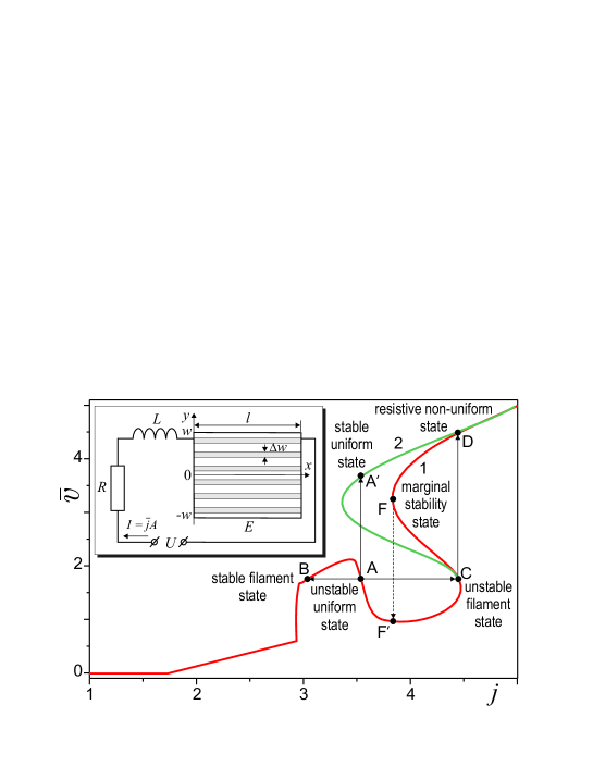
Figure 2: (Color online) Schematic VI curve of the superconductor for two different values of the hysteresis due to overheating. The more pronounced hysteresis loop (shown by the green solid line) corresponds to a larger value of the characteristic heat release. Inset: electrical circuit and the sample with filaments.

For small values of $|\partial j/\partial B|$, the solution of Eq. (3) can be found explicitly (with accuracy up to $|\beta^{2}|$): $\nu=-1-\gamma t_{0}/t_{s}$. It follows from this relation that the instability occurs only at the VI curve branch with NDR, if the drop of the voltage is large: $|\partial E/\partial j|>\rho_{c}$. The characteristic size of the arising filamentary structure is of the order of $\Delta w\propto w/|p_{1}|=w/\sqrt{|\gamma+t_{s}/t_{0}|}$. If $|\gamma t_{s}/t_{0}|\gg 1$, the filament width is small, $\Delta w\ll w$. Thus, the sample with NDR in the VI curve of $S$ type divides into small filaments with different current densities (in different dynamic flux flow phases III and IV) at $Rl/A\ll|\partial E/\partial j|$ and $L\ll 4\pi l/c^{2}A$. The obtained results are valid if $\rho_{c}^{-1}|\partial E/\partial j|\gg[(4\pi w/c)\partial j/\partial B]^{2}$. The instability occurs only if the left hand side of this last inequality is higher than unity; the right hand side is much smaller than 1 for the parameter range used above if $w<1$ mm. In the stationary inhomogeneous state that arises after development of the instability, the electric field should be uniform over the sample.

A more complex dynamics appears when the VI curve has simultaneously both NDR parts of $N$ and $S$ types (see Fig. 2). In this case, the filaments with higher current density $j_{C}$ are unstable if the system is far from the voltage-bias regime sch ; GMR . The instability of the filament with an $N$ type VI curve results in the switch of the filament into the overheated state GM D, giving rise to a non-uniform electric field distribution in the sample and, as a result, to non-zero $\dot{B}$. Thus, the state that appears after the instability develops is non-stationary. We consider two possible VI curves (type 1 red, type 2 green) shown in Fig. 2. In state D the flux lines move fast, which is accompanied with the acceleration of the flux flow in the lower-current filaments. In the nearly current-biased mode sch , if the VI curve is of type 2, the sample comes to the uniform stable state A^′ with the current density $j_{A}$. However, if the VI curve has the form shown in the (red) curve 1, the stable uniform state with the current density $j_{A}$ does not exist. In this case the high electric field state moves from point D to point F and falls down to a lower branch of the VI curve (point F^′). In this state, the electric field is also non-uniform and the lower and higher resistivity states will move towards A. However, this state is unstable and the cycle of transitions will be repeated ($A$ $\rightarrow$ $C$ $\rightarrow$ $D$ $\rightarrow$ $F$ $\rightarrow$ $F^{\prime}$ $\rightarrow$ $A$). Such a cyclical dynamic state could be realized in the form of flowing either stripes or resistive domain walls moving along the filaments.

It is important to stress that the described cyclical 5-step dynamics ($A$ $\rightarrow$ $C$ $\rightarrow$ $D$ $\rightarrow$ $F$ $\rightarrow$ $F^{\prime}$ $\rightarrow$ $A$) obtained for the IV curve having NDR of both $N$ and $S$ types cannot be realized for IV curves with either only N or only S type of NDR. The appearance of the non-stationary oscillatory regime for stationary external conditions is very unusual. This cyclic dynamics could be extended to different physical systems, e.g., plasmas or superconductors without artificial pins driven by a current flowing along the externally applied magnetic field brandt . Moreover, the predicted dynamical behavior (which can be generalized for several other systems, e.g., semiconductors) is potentially useful for the transformation of a dc input into either an ac-current or a voltage output which can be controlled by the parameters of the external circuit. In a broader sense, this general class of cyclic dynamics (ac output from dc input) is also found in other important nonlinear systems, like the dc Josephson effect.

In summary, for superconductors with periodic pinning arrays with certain pinning and heat transfer characteristics, we derive VI curves with NDR of $N$ type, $S$ type, or both. Complex dynamics and regimes including domain structures and filamentary instabilities appear when the VI curve has both $S$ and $N$ types of NDR. We analyzed the self-organized non-uniform dynamical regimes for these instabilities.

This work was supported in part by ARDA and NSA under AFOSR contract F49620-02-1-0334; and by the US NSF grant No. EIA-0130383.

References

- (1) See, e.g., E. Schöll, Nonequilibrium Phase Transitions in Semiconductors (Springer, Berlin, 1987); M.P. Shaw, V.V. Mitin, E. Schöll, H.L. Grubin, The Physics of Instabilities in Solid State Electron Devices (Plenum, London, 1992).
- (2) A.V. Gurevich, R.G. Mints, A.L. Rakhmanov, The Physics of Composite Superconductors (Begell, New York, 1997).
- (3) M.N. Kunchur et al., Phys. Rev. Lett. 84, 5204 (2000); 87, 177001 (2001).
- (4) A. Wehner et al., Phys. Rev. B63, 144511 (2001); O.M. Stoll et al., Phys. Rev. Lett. 81, 2994 (1998).
- (5) A.I. Larkin and Yu.N. Ovchinnikov, Zh. Eksp. Teor. Fiz. 68, 1915 (1975) [Sov. Phys. JETP 41, 960 (1976)].
- (6) S.G. Doettinger et al., Phys. Rev. Lett. 73, 1691 (1994); A.V. Samoilov et al., ibid 75, 4118 (1995); Z.L. Xiao et al., Phys. Rev. B 53, 15265 (1996).
- (7) F.F. Cap, Handbook on plasma instabilities (Academic, New York, 1976).
- (8) M. Tokunaga et al., Phys. Rev. Lett. 94, 157203 (2005).
- (9) M. Baert et al., Phys. Rev. Lett. 74, 3269 (1995); V.V. Moshchalkov et al., Phys. Rev. B 54, 7385 (1996).
- (10) J.E. Villegas et al., Science 302, 1188 (2003); Phys. Rev. B 68, 224504 (2003); M.I. Montero et al., Europhys. Lett. 63, 118 (2003).
- (11) A.M. Castellanos et al., Appl. Phys. Lett. 71, 962 (1997); R. Wördenweber et al., Phys. Rev. B 69, 184504 (2004).
- (12) L. Van Look et al., Phys. Rev. B 66, 214511 (2002).
- (13) A.V. Silhanek et al., Phys. Rev. B 67, 064502 (2003).
- (14) C. Reichhardt et al., Phys. Rev. Lett. 78, 2648 (1997); Phys. Rev. B58, 6534 (1998).
- (15) G. Blatter et al., Rev. Mod. Phys. 66, 1125 (1994); E.H. Brandt, Rep. Prog. Phys. 58, 1465 (1995).
- (16) A.V. Gurevich et al., Rev. Mod. Phys. 59, 941 (1987).
- (17) F. Nori, Science 271, 1373 (1996).
- (18) B.Y. Zhu et al., Phys. Rev. B 68, 014514 (2003); Physica (Amsterdam) 18E, 318 (2003); Physica (Amsterdam) 388-389C, 665 (2003); 404C, 260 (2004); Phys. Rev. Lett. 92, 180602 (2004).
- (19) V.R. Misko et al. (to be published).
- (20) See, e.g., E.H. Brandt, J. Low Temp. Phys. 39, 41 (1980).