Overdamped thermal ratchets in one and more dimensions. Kinesin transport and protein folding.

Abstract

The overdamped thermal ratchet driven by an external (Orstein-Uhlenbeck) noise is revisited. The ratchet we consider is unbounded in space and not necessarily periodic . We briefly discuss the conditions under which current is obtained by analyzing the corresponding Fokker-Planck equation and its lack of stationary states. Next, two examples in more than one dimension and related to biological systems are presented. First, a two-dimensional model of a “kinesin protein” on a “microtubule” is analyzed and, second, we suggest that a ratchet mechanism may be behind the folding of proteins; the latter is elaborated with a multidimensional ratchet model.

and

1 Introduction

The ratchet mechanism to produce directional current or motion has become a paradigm of the interplay of nonlinear phenomena with Brownian motion and external noise in mesoscopic systems[1, 2, 3]. We shall use the term “ratchet” for any conservative mechanical system that has an ingrained spatial asymmetry; a one-dimensional example is a particle in a saw-tooth like potential. Due to the potentiality of these systems to describe mesoscopic systems and their processes, such as biological ones[4], one should consider the ratchet to be immersed in a thermal bath, giving rise to Brownian motion. This adds dissipative and stochastic thermal forces that are related to each other through the fluctuation-dissipation theorem[5, 6]. As it was clearly pointed out by Feynman in his Lectures[7], the Second Law of Thermodynamics implies that a ratchet under the above conditions cannot generate directional motion. It is by now very well established that in order to obtain current or directional motion, it is indispensable to have the presence of an external unbiased time dependent force. This force can be deterministic, a so-called “rocking” ratchet, see Ref.[1], or stochastic in nature, see Ref.[8]. In any case, any of those forces should be of zero average in time in order not to produce any biased current; in the present article we shall be concerned with external stochastic forces only.

It is the opinion of the authors that the origin of the appearance of the current is not fully understood yet, although it is clear what the conditions are for its existence. In particular, a lot of attention has been devoted to the case in which the ratchet variable is periodic, such as an angle $\theta\in[0,2\pi]$, and many analytic and numerical results have been obtained[2, 9], yielding a clear picture of how current occurs in a stationary state. We believe the studies are not as exhaustive for the cases where the ratchet variable is not periodic, namely when the particle can move in all space, namely, when the position of the particle can take all real values, $x\in(-\infty,\infty)$. In this case, even in the absence of external forces, the system does not reach an stationary state[5]. One of the purposes of this article is to add to the understanding of the appearance of the current in the latter situation, by studying a novel non-periodic one-dimensional overdamped ratchet; this is done in Section 2.

Having established the conditions for the production of current in one dimension, we then proceed to the second purpose of the article and extend the model to more than one dimension in order to study two biology-related problems. One is the case of the motion of a kinesin protein on a microtubule, in Section 3, and the other is the process of protein folding in Section 4. The first has been studied already by several authors[10, 11] but here we consider a protein in two dimensions and the microtubule as a quasi-one dimensional structure. Our model of protein folding is at present speculative, and the idea is centered on the hypothesis that the energy landscape of the protein has a ratchet-like structure; by further assuming that there is an external agent that consumes energy, which could be the presence of chaperone proteins[12], one has all the ingredients to obtain directed motion. We shall show that, understanding by protein folding the search and finding of a target point or small section in the energy landscape, the ratchet mechanism is extremely fast with an almost perfect efficiency. An interesting consequence of this process is that the landscape need not have a funnel structure[13, 14].

2 Current in a one-dimensional overdamped ratchet

In this section we revisit the one-dimensional overdamped ratchet system, considering both periodic and non-periodic potentials. The main purpose here is to argue that the appearance of a current is a generic property of bounded asymmetric conservative systems, in interaction with a thermal bath, due to the presence of external (stochastic or deterministic) non-biased time dependent forces. That is, by showing that the absence of current without the external force must follow from the Second Law, we argue that there is nothing to prevent a current once the conditions required by the Second Law have been relaxed. The details of the numerical techniques we use can be found in Refs.[15, 16].

2.1 No current in the absence of external time-dependent forces

We initiate by writing down the the Langevin equation in the overdamped case for a particle subjected to a conservative potential $V(x)$, without an external time dependent force,

$$\gamma{dx\over dt}=-{\partial V\over\partial x}+f(t).$$ (1)

We consider a ratchet potential with a “quenched” random disorder both in the potential barriers and in the spatial periods, namely,

$$V(x) = -V_{0}^{(i)}\left[\sin\left(\frac{2\pi(x-y_{i})}{\lambda_{i}}\right)+\frac{2}{5}\sin\left(\frac{4\pi(x-y_{i})}{\lambda_{i}}\right)+\frac{1}{10}\sin\left(\frac{6\pi(x-y_{i})}{\lambda_{i}}\right)\right]$$ (2)

$$\>\>\>\>{\rm if}\>\>\>y_{i}\leq x<y_{i+1},$$

with $i$ taking all integer values and where the positions $y_{i}$ are chosen at random; $y_{0}$ is arbitrarily set equal to 0. Clearly, the spatial periods are given by $\lambda_{i}=y_{i+1}-y_{i}$. A typical form of the ratchet potential $V(x)$ is shown in Fig. 1. Note that this potential is not periodic. The usual periodic ratchet potential is $V_{0}^{(i)}\equiv V_{0}$ and $\lambda_{i}\equiv\lambda$ for all $i$[2].

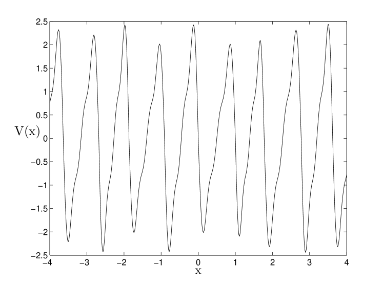
Figure 1: Ratchet potential with quenched random disorder both in the potential barriers and in the spatial periods. See Eq.(2).

Returning to the Langevin equation (1), $\gamma$ is the friction coefficient and $f(t)$ is the thermal force exerted by the thermal bath. The stochastic properties of this force are

$$\langle f(t)\rangle=0\>\>\>\>{\rm and}\>\>\>\>\langle f(t)f(t^{\prime})\rangle=2\gamma kT\delta(t-t^{\prime}).$$ (3)

It is further assumed that this process is Gaussian, so that Eqs.(3) suffice to completely specify the process $f(t)$. In the second equation $T$ is the temperature of the bath and the expression for the correlation of the force is the Fluctuation-Dissipation relation for this problem; it imposes detailed balance[5, 6].

Since the process $x(t)$ representing the position of the particle is Markovian, then, knowledge of the conditional probability distribution $\rho(x,t|x_{0})$ is enough to determine the process. It can be shown that this function obeys the following Fokker-Planck equation[5],

$${\partial\rho(x,t)\over\partial t}={1\over\gamma}{\partial\over\partial x}\left({\partial V\over dx}+kT{\partial\over\partial x}\right)\rho(x,t),$$ (4)

supplemented by the initial condition $\rho(x,0|x_{0})=\delta(x-x_{0})$.

In this discussion we are considering that the particle can move in all space, namely, $-\infty<x<\infty$. Thus, the normalization of the distribution,

$$\int_{-\infty}^{\infty}\rho(x,t)\>dx=1,$$ (5)

imposes the boundary conditions

$$\rho(x,t)\to 0\>\>\>\>{\rm for}\>\>\>\>x\to\pm\infty.$$ (6)

The Fokker-Planck equation, Eq.(4), is a continuity equation for the probability distribution. Therefore, one can read off the probability density current,

$$j(x,t)=-{1\over\gamma}{\partial V\over\partial x}\rho(x,t)-{kT\over\gamma}{\partial\rho(x,t)\over\partial x}.$$ (7)

We may define the “total” current as,

$$J(t) = \int_{-\infty}^{\infty}j(x,t)\>dx$$ (8)

$$= -{1\over\gamma}\langle{\partial V\over\partial x}\rangle$$

$$= {d\over dt}\langle x(t)\rangle,$$

where the last two lines follow from the definition of the density current and the Fokker-Planck equation, Eqs.(7) and (4).

If there exists a stationary distribution, $\rho_{s}(x)$, then detailed balance means that the stationary density current vanishes, $j_{s}(x)=0$, and therefore that the stationary distribution is

$$\rho_{s}\sim e^{-\beta V(x)},$$ (9)

with $\beta=1/kT$. Further, if $\rho(x,t)$ is not the stationary distribution, then, detailed balance implies that as $t\to\infty$, such a distribution approaches the stationary one. This is equivalent to the $H$-theorem.

In the context of ratchet-like potentials, one is faced with potentials that are bounded, that is, $V_{1}\leq V(x)\leq V_{2}$, for all $x$. Thus, strictly speaking, a stationary distribution cannot be reached[5]. However, it is clear that stationarity is achieved in the following sense,

$$\lim_{t\to\infty}{\rho(x,t)\over\rho(x^{\prime},t)}=e^{-\beta(V(x)-V(x^{\prime}))}.$$ (10)

Therefore, it must be true that, in the above sense, the probability density current $j(x,t)$ and the total current $J(t)$ must vanish as $t\to\infty$. However, this does not suffice to prevent an arbitrary current or displacement of the particle, as is routinely asserted in essentially all articles dealing with this problem. The main point that we want to emphasize here is that, since detailed balance is in accordance with the Second Law of Thermodynamics, the total current $J(t)$ must be bounded for all times. Using Eq.(8), this can be more precisely written as the following requirement,

$$|\langle x(t)\rangle-x_{0}|=\left|\int_{0}^{t}\>d\tau\>J(\tau)\right|<\bar{\lambda}(x_{0}),$$ (11)

where $x_{0}$ is the initial position of the particle and $\bar{\lambda}(x_{0})$ is the distance between the adjacent local maxima of the potential where the particle was initially at $x=x_{0}$. We have exhaustively numerically verified that this holds for ratchet potentials such as those ones in Fig. 1, and the results are exemplified in Fig. 2.

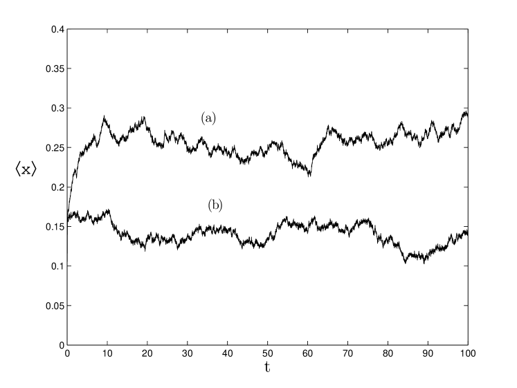
Figure 2: Average position of the particle $\langle x(t)\rangle$ as a function of time, for the case of no external time-dependent force, see Eq.(1). (a) For a disordered ratchet potential. (b) For a periodic ratchet potential. In both cases the initial condition is $x=-0.04$. Note that the particle, on the average, never leaves the well where it started, see Fig. 1.

For ratchet potentials this means that on the average the particle cannot leave the local well where it was initially; if it did, nothing would prevent the particle to “jump” to another well, and so on, thus moving an arbitrary distance. In other words, Eq.(11) expresses that fact that it is not possible to obtain a current that, on the average, could generate motion that would transport the particle farther than its initial well. Otherwise, this would yield the possibility to perform work on some external load or agent[17] violating Kelvin’s statement of the Second Law: “A transformation whose only final result is to transform into work heat extracted from a source which is at the same temperature throughout is impossible”[18]. In the opinion of the authors, this is what Feynman, in his Lectures[7], wants to convey in his discussion of a ratchet engine.

It is important to stress that we consider high enough temperatures so that the particle, even though it does not move on the average, it does perform normal diffusion. This is shown in Fig. 3.

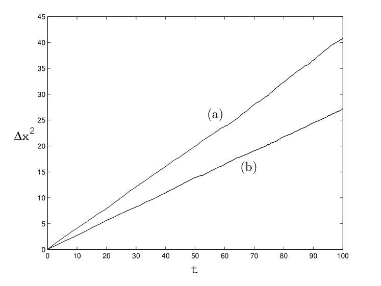
Figure 3: Second moment of the particle position distribution $\Delta x^{2}=\langle x^{2}(t)\rangle-\langle x(t)\rangle^{2}$ as a function of time, for the case of no external time-dependent force, see Eq.(1). (a) For a disordered ratchet potential. (b) For a periodic ratchet potential. As discussed in the text the particle performs normal diffusion.

2.2 Current in the presence of an external time-dependent force

In the presence of a time-dependent external force $F(t)$, the Langevin equation reads,

$$\gamma{dx\over dt}=-{\partial V\over\partial x}+f(t)+F(t),$$ (12)

where the thermal force $f(t)$ obeys the same properties as before, see Eqs.(3). As an example, the external force $F(t)$ may be generated by an Orstein-Uhlenbeck process

$$\tau_{0}{dF\over dt}=-F+\zeta(t),$$ (13)

with $\zeta(t)$ a given Gaussian, white, stochastic process:

$$\langle\zeta(t)\rangle=0\>\>\>\>\langle\zeta(t)\zeta(t^{\prime})\rangle=f_{0}^{2}\delta(t-t^{\prime}).$$ (14)

The parameters $\tau_{0}$ and $f_{0}$ determine the process. The first one is the correlation time for $F(t)$ and $f_{0}$ is a measure of its strength. In order to avoid any bias by this force, one must consider the initial condition $F(0)=0$.

Equations (12), (3), (13) and (14) are equivalent to the following bivariate Fokker-Planck equation[9],

$${\partial W(x,F,t)\over\partial t} = {1\over\gamma}{\partial\over\partial x}\left(-F+{\partial V\over\partial x}+kT{\partial\over\partial x}\right)W(x,F,t)$$ (15)

$$+{1\over\tau_{0}}{\partial\over\partial F}\left(F+{f_{0}^{2}\over 2\tau_{0}}{\partial\over\partial x}\right)W(x,F,t),$$

where $W(x,F,t|x_{0},0)$ is the conditional probability distribution to find values $x$ and $F$ for the corresponding stochastic variables, given that at $t=0$, $x=x_{0}$ and $F=0$. Initially, it is $W(x,F,0|x_{0},0)=\delta(x-x_{0})\delta(F)$.

By simple inspection we find that, even if a stationary distribution $W_{s}(x,F)$ exists, equation (15) does not obey detailed balance. The “offending” term is

$${1\over\gamma}{\partial\over\partial x}(-FW(x,F,t)).$$ (16)

This, of course, only means that $F(t)$ is “external”. Namely, $F$ acts on $x$ but not the opposite, Thus, there is no mechanism to establish equilibrium among the particle, the thermal bath and the external agent. Therefore, the system can withdraw energy from the external source and generate motion. In other words, there is nothing to prevent the total current from taking any value different from zero:

$$J(t)=-{1\over\gamma}\int_{-\infty}^{\infty}dx\int_{-\infty}^{\infty}dF\>W(x,F,t){\partial V(x)\over\partial x}\neq 0,$$ (17)

or

$$J(t)={d\over dt}\langle x(t)\rangle\neq 0.$$ (18)

In other words, in this case the Second Law does not impose any restriction on the appearance of a current. The Second Law will now impose restrictions on the efficiency of the process but that is not discussed here. Of course, if the potential $V(x)$ does have a “left-right” symmetry, the current vanishes as one should expect.

In Fig. 4 we exemplify the appearance of a current, both for the disordered potential and for the periodic one. On top of the current, the particle also performs normal diffusion, i.e. for long times $<x^{2}(t)>-<x(t)>^{2}\sim Dt$.

Figure 4: Average position $\langle x(t)\rangle$ as a function of time in the presence of an external time-dependent force. (a) For a disordered ratchet potential. (b) For a periodic ratchet potential.

3 A two-dimensional “kinesin on a microtubule” model

During the last few years there has been an increasing interest in studying the statistical behavior of the transport phenomena inside the cell carried out by protein motors and it has been proposed by several authors that ratchet models may be relevant in the description of these processes[1, 2, 8, 9, 10, 19]. Protein motors are responsible for carrying diverse kind of vesicles from one site to another in the cell in a much more efficient way than the obtained by simple diffusion[12]. To accomplish this task they consume chemical energy, usually stored in the form of adenosine-triphosphate (ATP), to convert it into mechanical motion [2]. Due to their dimensions, the erratic collisions with the solvent molecules represent a non negligible contribution to the protein motors dynamics and appear in the form of friction and thermal stochastic forces. This is why they are also called Brownian motors or molecular motors[4].

Molecular motors, as kinesin and dynein, present directed motion only when they are attached to microtubules, otherwise they perform standard Brownian motion. It has been also observed that they do not hydrolyze ATP at an appreciable rate unless they are attached[2]. Experimental observations of kinesin and dynein motion on microtubules[20] have shown that kinesins move mainly along one single protofilament, while dyneins visit often several protofilaments. One important characteristic of the microtubules is that they have an intrinsically periodic and asymmetric structure[12].

Most of the models motivated by these experimental results were initially restricted to the one dimensional case but it has become clear that more dimensions are needed[11, 21, 22, 23, 24, 25, 26, 27, 28, 29]. Some of these works[28, 29] approach the problem imposing ad hoc asymmetric probabilities thus obtaining transport. The others use Langevin equations and, in particular, those in Refs.[11, 21, 22, 23] have introduced more detailed models to understand the particular behavior of kinesin in microtubules.

As an step forward in the description of these processes, we are considering here a model for a kinesin on a microtubule as a ratchet in a two dimensional space, immersed in a thermal dissipative bath, and subjected to an external force of zero mean varying stochastically in time. At present we study general statistical properties of the model; a more detailed study and its comparison with real kinesin proteins will be presented elsewhere. Nevertheless, the results shown here resemble qualitatively what is observed in actual experiments with motor proteins and microtubules[12].

In order to model the interaction forces between the motor protein and the microtubule a two-dimensional potential is proposed, whose shape resembles a long attractive filament (or channel) with a typical ratchet structure inside on the longitudinal direction, as shown in Fig. 5.

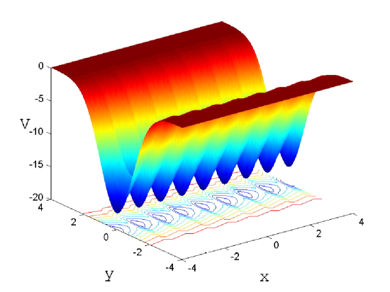
Figure 5: Two-dimensional potential with an infinite attractive filament (or channel) along the $x$ coordinate and a ratchet structure inside of it. The attractive filament has a mean depth of $V_{1}=15$ and a width determined by $\sigma=2$, while $\lambda=1$ represents the period of the ratchet and $V_{0}=2$ its amplitude. The longitudinal projection of this potential is similar as the used in one dimension models. In the transversal direction, $-\infty<y<\infty$.

The potential $V(x,y)$, called for simplicity the filament or microtubule potential, is given by the following function

$$V(x,y)=-e^{-y^{2}/\sigma^{2}}\left[V_{1}+V_{0}\left(\sin\left(\frac{2\pi x}{\lambda}\right)+\frac{4}{10}\sin\left(\frac{4\pi x}{\lambda}\right)+\frac{2}{10}\sin\left(\frac{6\pi x}{\lambda}\right)\right)\right],$$ (19)

where $V_{1}$ is the mean depth of the attractive filament and its width is determined by $\sigma$; $\lambda$ represents the period of the ratchet and $V_{0}$ the amplitude. The system is immersed in a thermal bath at temperature $T$ and there is present an external random force with zero mean that represents in the model the consumption of ATP by the protein motor. Depending on the temperature of the bath and on the statistical properties of the external force, the particle may be inside or outside the microtubule, i.e. $|y|\leq\sigma$ or $|y|>\sigma$ . Inside, it will feel the effect of the ratchet potential and may generate directed motion; outside, it will perform free Brownian motion.

The dynamics of the model are represented by the following coupled Langevin equations for a Brownian particle moving in an $x-y$ coordinate system:

$$\gamma\frac{dx}{dt}=-\frac{\partial V(x,y)}{\partial x}+f_{x}(t)+F_{x}(t),$$ (20)

and

$$\gamma\frac{dy}{dt}=-\frac{\partial V(x,y)}{\partial y}+f_{y}(t)+F_{y}(t),$$ (21)

where $\gamma$ is the friction coefficient and $f_{i}(t)$, with $i=x,y$, is the force exerted by the thermal bath. The stochastic properties of this force are

$$\langle f_{i}(t)\rangle=0\>\>\>\>{\rm and}\>\>\>\>\langle f_{i}(t)f_{j}(t^{\prime})\rangle=2\gamma kT\delta(t-t^{\prime})\delta_{ij}.$$ (22)

It is further assumed that these processes are Gaussian. The external force is $F_{i}(t)$ with $i=x,y$. Due to the lack of information with respect to the actual statistical properties of ATP consumption by the kinesin, and which is one the main difficulties to make precise predictions, we have decided to employ a stochastic force generated by an Ornstein-Uhlenbeck process

$$\tau_{0}\frac{dF_{i}(t)}{dt}=-F_{i}(t)+\zeta_{i}(t),$$ (23)

with $\zeta_{i}(t)$ a given Gaussian, white, stochastic process

$$\langle\zeta_{i}(t)\rangle=0\>\>\>\>{\rm and}\>\>\>\>\langle\zeta_{i}(t)\zeta_{j}(t^{\prime})\rangle=f_{o}^{2}\delta(t-t^{\prime})\delta_{ij}.$$ (24)

The parameters $\tau_{0}$ and $f_{0}$ determine the process and represent the correlation time and the magnitude of the external force, respectively. As it can be observed, the relations for $f_{i}(t)$ and $F_{i}(t)$ are exactly the same for both directions and they are ruled by the same parameters. In consequence, they act isotropically. However, each of them arise from an independent Gaussian noise, and thus, there is no correlation among them.

We now present the main statistical properties of this model. In all the results presented here the initial conditions are $x(0)=y(0)=0$. Variations of the different parameters, a thorough description of the behavior of the first and second moments of the position distribution of the particle, as well as a comparison with actual motor proteins, cannot be presented here due to the briefness of this report and will be discussed elsewhere.

As one should expect, the presence of the external time dependent force produces a net current along the $x$ direction due to the asymmetric properties of the ratchet inside the filament. In the present case, the total current is a two-dimensional vector,

$$\vec{J}(t)=J_{x}(t)\hat{i}+J_{y}(t)\hat{j}=\frac{d}{dt}\langle x(t)\rangle\hat{i}+\frac{d}{dt}\langle y(t)\rangle\hat{j}.$$ (25)

In Fig.6 we show the average $x$-position of the particle as a function of time, the current $J_{x}(t)$ being the derivative of such a curve. The current along $y$ is zero, $J_{y}(t)=0$, as expected.

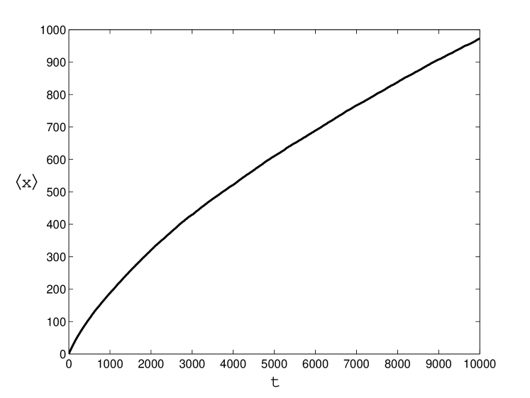
Figure 6: Average $x$-position of the particle as a function of time.

The current occurs, however, in an interesting manner. First, we realize that the particle feels the effect of the ratchet only when it is inside the filament. Outside, it performs diffusive standard Brownian motion. The net result is that the current tends, asymptotically and very slowly, towards zero. However, for any finite amount of time, the current is different from zero. Thus, a net transport is always realized. Another form of saying this is that, even though the particle may stay a long time outside the filament, it effectively has directional motion since it eventually returns to it. This is better seen in Fig.7, where we present four “snapshots” of the position probability distribution $\rho(x,y,t)$ for different times, and obtained from 2000 realizations of the process. The distribution acquires an arrow-like structure because of the ratchet within the filament and the centroid moves always to larger values of $x$, i.e. the distribution appears to be dragged by the filament.

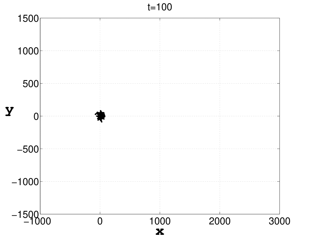
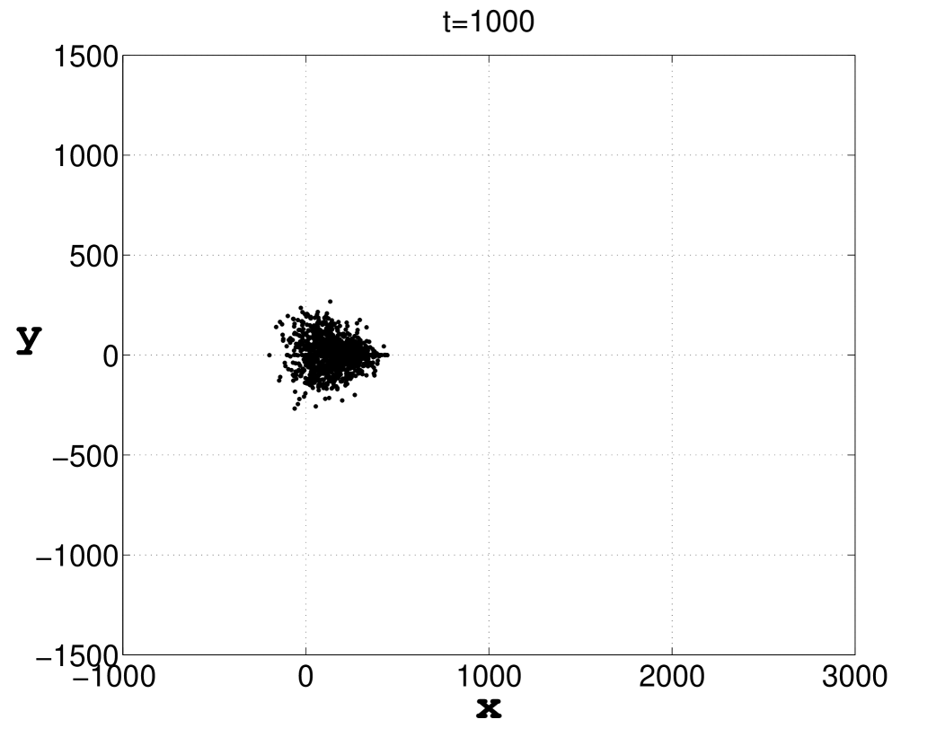
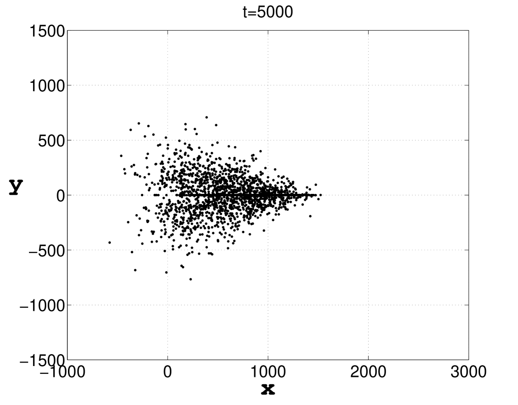
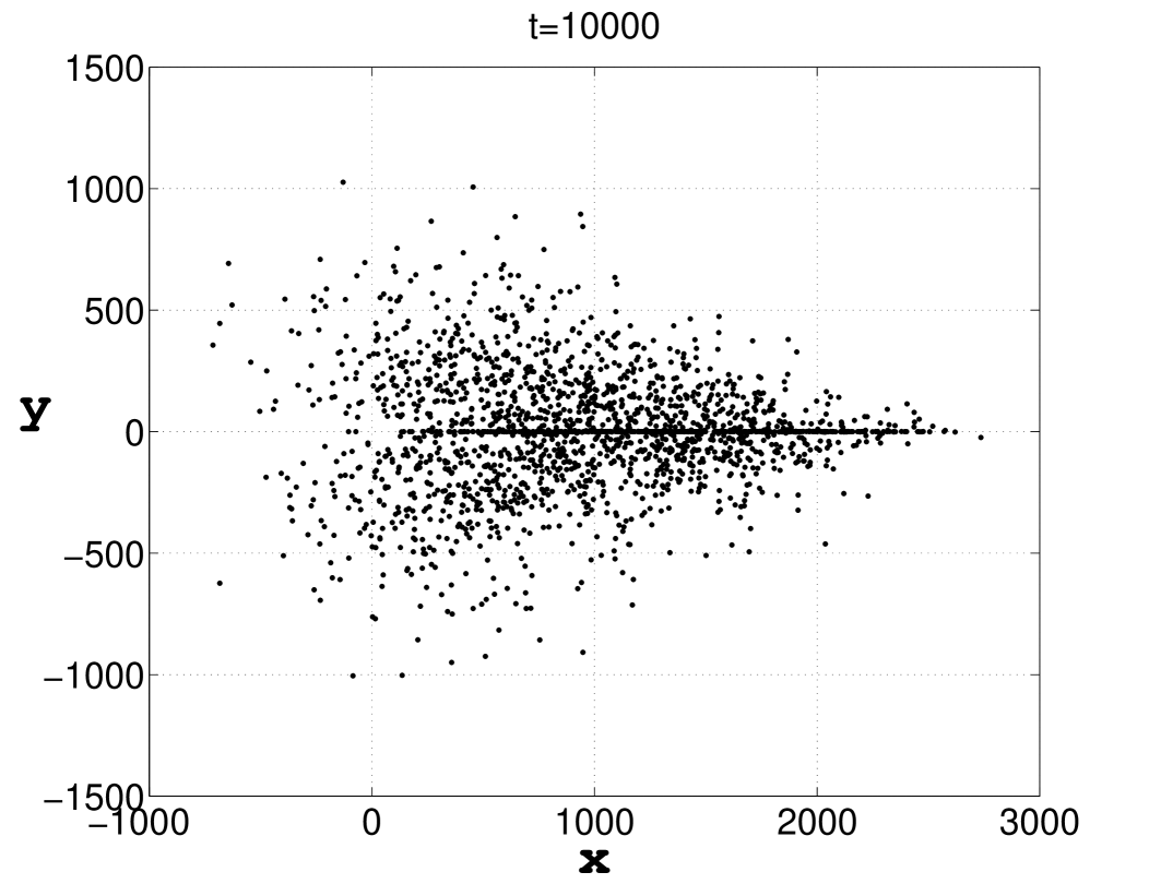
Figure 7: Snapshots of the position probability distribution $\rho(x,y,t)$ for four different times, obtained from 2000 realizations of the process.

The shape of the position distribution $\rho(x,y,t)$ suggests also a peculiar behavior of its second moment,

$$\Delta r^{2} = \Delta x^{2}+\Delta y^{2}$$ (26)

$$= \left(\langle x^{2}\rangle-\langle x\rangle^{2}\right)+\left(\langle y^{2}\rangle-\langle y\rangle^{2}\right).$$

In Fig. 8 we show these three deviations. The total second moment $\Delta r^{2}$ follows a power law $t^{\alpha}$ with $\alpha\approx 1.5$ after $t\approx 100$ time units. That is, the system effectively presents superdiffusion, in contrast to the one-dimensional case where it is always normal diffusion. The super diffusive behavior is also present in the $x$-direction, while in the $y$ direction the diffusion is normal.

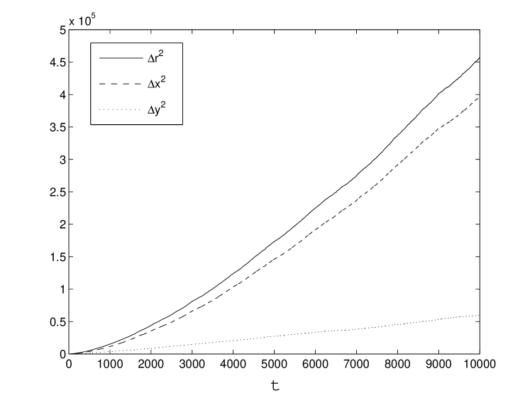
Figure 8: Total second moment $\Delta r^{2}$ and its components in $x$ and $y$, see Eq.(25), as a function of time. Note that both $\Delta r^{2}$ and $\Delta x^{2}$ show superdiffusive behavior, while $\Delta y^{2}$ shows normal diffusion.

The explanation for this behavior appears to be simple: When the particle is bound to the filament it feels the effect of the ratchet and tends to move preferentially in the positive $x$ direction. When it is outside of the channel performs a normal random walk, with normal diffusion, but it does not move preferentially to any direction. Thus, for those times when it is outside the filament, even though appears statistically to be dragged by the filament as mentioned above, the particle lags behind the centroid, hence effectively producing a wider distribution and a larger second moment. It is interesting to point out that the superdiffusive behavior is a consequence of “standard” noises coupled to a highly nonlinear process and does not arise from an exotic stochastic process[30].

4 A ratchet mechanism behind protein folding?

Following the classical work of Anfinsen[31] on protein folding, Levinthal[32] argued that if the multidimensional (free) energy landscape had a “golf course” like shape, with the hole being the protein native state, it would take essentially forever for a protein to fold correctly, provided the search were performed at random, namely, by Brownian motion. Since proteins in vivo fold extremely fast and efficiently[12] the concept of a funneled energy landscape was developed[13, 14], with the further possibility of folding pathways in which the protein folds following a path towards or within the funnel leading to the native state. But very importantly, the process being driven essentially by free energy differences, that is, by “falling” into the state of lowest free energy. This idea has been central in the study of protein folding and we do not pretend to review all the advances made by the many groups working on this field[33] nor to point out any possible pitfalls of the theories. Rather, we would like to point out an alternative way out to the so-called Levinthal paradox, without necessarily requiring a funnel leading to the native state. We shall appeal to a ratchet mechanism for the process of protein folding. This model requires, in addition to having a ratchet-like energy landscape as we discuss below, that the folding is a non-equilibrium process being driven by an “external” source.

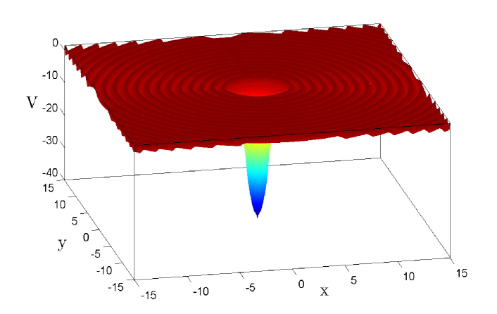
Figure 9: Two-dimensional “free energy” landscape of a protein, see Eq.(27). The landscape is flat on the average with a ratchet-like structure on top of it. The deep well in the center is the “native” structure of the protein.

The model consists of a “particle” moving in a multidimensional space, the coordinates representing the different configurations of a protein, or effective degrees of freedom[36]. The particle is affected by a conservative ratchet potential which maybe flat on the average (i.e. no need of a funnel) and with a “small and deep enough hole” representing the native state. On top of the average potential there is an asymmetry that makes the potential toward the native state, different than in the opposite direction. Fig. 9 is a two-dimensional example for visualization, but we have realized many multidimensional potentials with the same type of “toward-away” asymmetry, see below. Although we cannot justify the existence of such a potential, one may argue that the regularity specially in the secondary structures, at least at first order, suggest a kind of “universal” regular potential. Our proposal, undoubtedly not quite justified, is that such a regularity may have a ratchet-like form; after all, any coiling structure has an asymmetry since it distinguishes between “right” and “left”. The presence of the thermal bath needs no justification and simply represents the effect of a viscous environment at a fixed temperature. With only the last two ingredients, the ratchet potential and the bath, the “particle” will obey Levinthal paradox and would not find its way in a reasonable time, specially in a multidimensional space. However, if the there is an external source of energy, with random properties and zero bias, acting on the particle, the latter will definitely find its way toward the native state and, on the average, could do so in a short time. The efficiency of the process, of course, will depend on the values of the different parameters. What is the origin of the external source? We may generically argue that processes in living organisms are through states of non-equilibrium with all sorts of gradients of different physical properties, and that the maintenance of those gradients may be traced back to the consumption of ATP. In a more specific way, although it is not clear that occurs in all proteins, it is known that many proteins fold assisted by chaperone proteins, which in turn, consume ATP[34]. Thus, the proposed mechanism requires the presence of an external source, which in our opinion, is physically appealing since Life needs such a source for occurring as required by the Second Law. Nonetheless, we cannot say exactly what the mechanism is at the level of the protein.

The mathematical model is, therefore, a multidimensional version of Eqs.(20) and (21) for the kinesin-on-a-microtubule model, but now the ratchet potential has an overall ( topologically equivalent) spherical symmetry, with a “towards-away” asymmetry. For the numerical results we present below we consider periodic potentials such as the following,

$$V(x_{1},x_{2},\dots,x_{d}) = V_{0}\left[\sin(2\pi r/\lambda)+a\sin(4\pi r/\lambda)+b\sin(6\pi r/\lambda)\right]$$ (27)

$$-V_{1}e^{-cr^{2}}.$$

where $d$ is the dimension of the space, namely, the number of effective degrees of freedom of the protein; $r=(x_{1}^{2}+x_{2}^{2}+\cdots+x_{d}^{2})^{1/2}$; and $a$, $b$ , $c$, $V_{0}$ and $V_{1}$ real positive numbers. The last term in Eq.(27) represents the “hole” of the native state. We want to insist that the ratchet potential need not be periodic, that is, the saw-tooth structure can have “quenched” random distances between maxima and minima, such as in the one-dimensional case, see Fig. 2. Furthermore, the landscape does not have to be flat, namely, it can have valleys and peaks, wider and higher or lower than the average peaks of the ratchet, and the particle can still climb over the peaks provided they are not above the stall load of the ratchet[17]. Full analysis of these cases are beyond the briefness of this report and it will be presented elsewhere.

Fig.10 shows a typical example of the many different cases we have analyzed. It corresponds to a “protein” with 6 degrees of freedom. We show the average evolution of the protein coordinates $x_{i}(t)$, with $i=1,2,\dots,6$ over 100 runs for the same initial condition. In the presence of the external force, and for those parameters, we found more than 95$\%$ “folding”, namely, the particle reached the “native” state in the arbitrary maximum time of 15000 units. The average time of folding can be read off the graph and corresponds to 4000 unit times approximately, very short even in CPU time scales. When the external field was turned off, needles to say, we found 0$\%$ “folding”, and we believe it will essentially never find its way no matter how long we run the program.

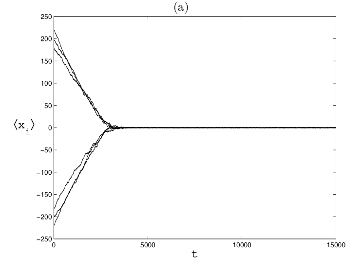
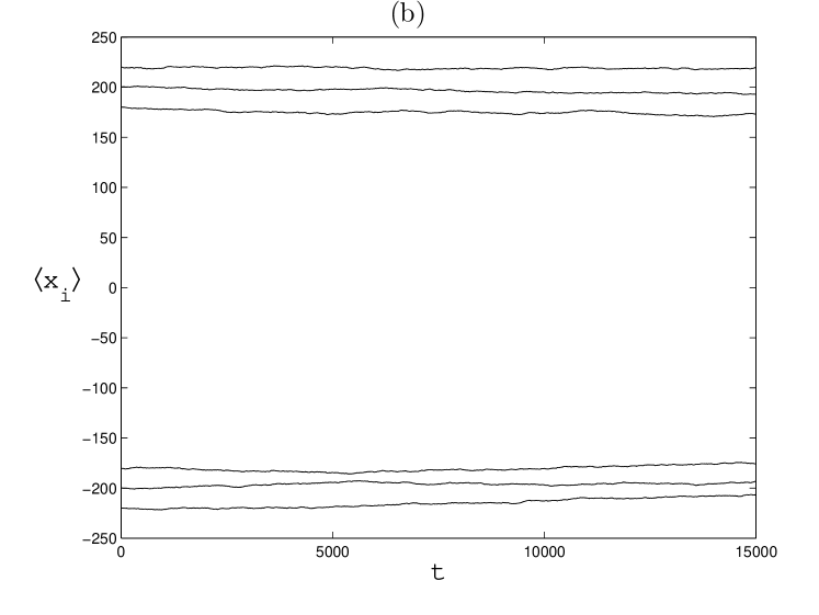
Figure 10: Average particle position $\langle x_{i}(t)\rangle$ in a six-dimensional space, $i=1,\dots,6$, as a function of time for 100 realizations and same initial conditions. The spatial period of the ratchet is $\lambda=1$. (a) In the presence of the external time dependent force, the “protein” folds. (b) In the absence of the external time dependent force, the “protein” essentially never folds.

5 Remarks

In this article we have revisited overdamped ratchet systems in one dimension and extended it to several dimensions in order to study biology related systems. For the case of one dimension we analyzed a novel disordered ratchet for the purpose of making explicit the fact that the space in which the systems move do not correspond to a periodic variable, as it is routinely done in the literature. For these systems, strictly speaking, do not exist a stationary state. The main result that we want to stress here is the fact that, in the absence of external time dependent forces, stochastic or deterministic, there cannot be a current for all times and not only as an asymptotic condition. This is a requirement of the Second Law. Once there is an external time dependent force, and the system shows an intrinsic asymmetry, such as a “left-right” one, there is nothing to prevent a current. The Second Law now acts by setting limits for the amount of work released, namely on the efficiency of the process. We did not address the latter limits although several workers have discussed this point[17].

The ratchet mechanism has become a potential candidate for many biological process, since, on the one hand resembles a thermal engine at a mesoscopic level, but on the other it does not appear to need a specific design such as the man-made engines. That is, by its inherent capacity to deliver work in the form of directional motion, one may be prompted to use it as a model in somewhat obvious biological situations in which a transport process, of some kind, is present. This has been the case of the motion of kinesin proteins on microtubules, where the protein appears to truly “walk” using ATP as the necessary input energy; there are other cases where ratchets have been used as models of intracellular motion, or as molecular motors, such as in the mitosis of the cell[35]. Granted, all the models are still at a very premature level of comparison with actual situations, mainly because the complicated biochemical processes involved in real life can hardly be thought to be described by systems with one or two degrees of freedom. Nevertheless, we believe it is worthwhile to keep exploring these models not only by its potential relevance in biological systems but for their own sake. Here, we have presented a two dimensional model of a kinesin in the presence of a quasi one-dimensional microtubule. The typical walks of the particle, wandering around until they hit the microtubule and then directionally moving, show a striking similarity with actual kinesin motion, as seen in videos of these systems[37]. Although one can always try to fit these simple results to known conditions, such as speed of kinesin walks or the energy released by the consumption of ATP, we believe further research is needed in two aspects of the model: first, we must confidently know how to relate the ratchet potential with the actual periodic structure of the microtubule and the form in which the protein attaches to it, and second, how to describe the consumption of ATP by means of an appropriate statistical process.

The third section of this article on considering protein folding as being driven by a ratchet mechanism is highly speculative, but we believe it is worthwhile to pursue it because, again, protein folding appears as a process with directional motion. Traditionally, this process has been thought to be driven by free energy differences leading towards a minimum, similarly to a chemical reaction[13], and thus the idea of a funnel in the free energy landscape of the protein. The presence of catalyzers and/or chaperone proteins may accelerate this process and their presence is welcome in the theory. Here, by following the idea that Life processes consume energy to yield their products, similarly to a man-made thermal engine, we have speculated that protein folding is driven by an “engine” in which the protein itself is part of it. This now makes a necessity the presence of choperones and/or catalyzers that in turn consume energy. At this moment, the hardest part to justify in our model is the ratchet structure of the energy landscape, and the best that we can say is that it is motivating to see that the secondary structure of proteins is universally made of $\alpha$-helices and $\beta$-sheets, structures with certain periodicity and asymmetry. On the other hand, we do not have evidence neither pro nor con that a ratchet structure is present since this would have to be seen in the highly multidimensional energy landscape. As mentioned before, the “folding” with this mechanism does not need a funnel, but of course, the interplay of both properties would make the process even more efficient. The simulations that we have performed, so far up to a landscape in 6 dimensions, are extremely encouraging since they can easily be tuned to a very fast and almost 100 $\%$ “folding”. Extending to an arbitrary number of dimensions only requires longer computer time and, at present, does not add anything fundamentally different. What is really needed is the actual form of an energy landscape, a hard problem with many researchers very much interested in it. However, without yet knowing the actual form of an energy landscape in its many dimensions, we can make models in which the ratchet is not periodic and in which the landscape have valleys and peaks to test the efficiency of the search for the “native” state. We shall present those results in future contributions.

References

- [1] M. Magnasco, Phys. Rev. Lett. 71 (1993) 1477.
- [2] P. Reimann, Phys. Rep. 2 (2001) 237, and references therein.
- [3] P. Hanggi, F. Marchesoni, and F. Nori, Ann. Phys. 14 (2005) 51, and references therein.
- [4] R.D. Astumian and P. Hanggi, Phys. Today 55 (2002) 33.
- [5] N.G. van Kampen, Stochastic Processes in Physics and Chemistry, North Holland, Amsterdam, 1981.
- [6] H. Risken, The Fokker-Planck equation, Springer, Berlin, 1984.
- [7] R.P. Feynman, R.B. Leighton, and M. Sands, The Feynman Lectures on Physics, Vol. I, Addison Wesley, Reading, 1963.
- [8] C.R. Doering, W. Horsthemke, and J. Riordan, Phys. Rev. Lett. 72 (1994) 2984.
- [9] R. Bartussek, P. Reimann, and P. Hanggi, Phys. Rev. Lett. 76 (1996) 1166.
- [10] R.D. Astumian and M. Bier, Phys. Rev. Lett. 72 (1994) 1766.
- [11] see J.L. Mateos in this issue.
- [12] B. Alberts, A. Johnson, J. Lewis, M. Raff, K. Roberts, and P. Walter, The molecular biology of the cell, Garland, New York, (2002).
- [13] J.D. Bryngelson, J.N. Onuchic, N.D. Socci, and P.G. Wolynes, Proteins: Struct., Funct., Genet. 21 (1995) 167.
- [14] K. Dill, S. Bromberg, K. Yue, K.M. Fiebig, D.P. Yee, P.D. Thomas, and H.S. Chan, Protein Sci. 4 (1995) 561.
- [15] L.A. Ibarra-Bracamontes and V. Romero-Rochin, Phys. Rev. E 56 (1997) 4048.
- [16] L. Viana and V. Romero-Rochin, Physica D 168 (2002) 193.
- [17] J.M.R. Parrondo and B.J. de Cisneros, Appl. Phys. A 75 (2002) 179.
- [18] E. Fermi, Thermodynamics, Dover, New York, 1956.
- [19] F. Julicher, A. Ajdari, J.P. Prost, Rev. Mod. Phys. 69 (1997) 1269.
- [20] Z. Wang, S. Khan, M.P. Sheetz, Biophys. J. 69 (1995) 2011.
- [21] S.Cilla and L.M. Floría, Il Nuovo Cimento, 20 (1998) 1761.
- [22] T.J. Zhao, Y.Z. Zhuo, Y. Zhan, Q. Yi, T.G. Cao, Mod. Phys. Lett. B 16 (2002) 999.
- [23] J. Middleton, J. A. Tuszynski, CRM Proceedings and Lecture Notes. 39 (2004) 251.
- [24] M. Kostur, L. Schimansky-Geier, Phys. Lett. A 265 (2000) 337.
- [25] J.D. Bao Phys. Rev. E 62 (2000) 4606.
- [26] J.D. Bao Phys. Rev. E 63 (2001) 061112.
- [27] R. Eichhorn, P. Reimann, P.Hanggi, Physica A 325 (2003) 101.
- [28] R. Lipowsky, S. Klumpp, T. M. Nieuwenhuizen, Phys. Rev. Lett. 87 (2001) 108101.
- [29] T. M. Nieuwenhuizen, S. Klumpp, R. Lipowsky, 58 (2002) 468.
- [30] J.M. Sancho, A.M. Lacasta, K. Lindenberg, I.M. Sokolov, and A.H. Romero, Phys. Rev. Lett. 92 (2004) 250601.
- [31] C.B. Anfinsen, E. Haber, M. Sela, and F.H. White, Proc. Natl. Acad. Sci. 47 (1961) 1309.
- [32] As quoted in Ref.[13].
- [33] The number of researchers working on protein folding is enormous, see the web page http://www.fccc.edu/research/labs/roder/foldinggroups.html.
- [34] R.J. Ellis and F.-U. Hartl, FASEB J. 10 (1996) 20.
- [35] F. Gibbons, J.-F. Chauwin, M. Despósito, and J.V. José, Biophys. J. 80 (2001) 2515.
- [36] The multidimensional free energy landscape may already have the information that the system is immersed in water. That is, the interaction potential should have all effective interactions due to the hydrophilic or hydrophobic properties of the different aminoacids.
- [37] See the videos in the DVD disk accompanying the book by Alberts et al., Ref.[12].