Global Optimization, the Gaussian Ensemble, and Universal Ensemble Equivalence

Abstract

Given a constrained minimization problem, under what conditions does there exist a related, unconstrained problem having the same minimum points? This basic question in global optimization motivates this paper, which answers it from the viewpoint of statistical mechanics. In this context, it reduces to the fundamental question of the equivalence and nonequivalence of ensembles, which is analyzed using the theory of large deviations and the theory of convex functions.

In a 2000 paper appearing in the Journal of Statistical Physics, we gave necessary and sufficient conditions for ensemble equivalence and nonequivalence in terms of support and concavity properties of the microcanonical entropy. In later research we significantly extended those results by introducing a class of Gaussian ensembles, which are obtained from the canonical ensemble by adding an exponential factor involving a quadratic function of the Hamiltonian. The present paper is an overview of our work on this topic. Our most important discovery is that even when the microcanonical and canonical ensembles are not equivalent, one can often find a Gaussian ensemble that satisfies a strong form of equivalence with the microcanonical ensemble known as universal equivalence. When translated back into optimization theory, this implies that an unconstrained minimization problem involving a Lagrange multiplier and a quadratic penalty function has the same minimum points as the original constrained problem.

The results on ensemble equivalence discussed in this paper are illustrated in the context of the Curie-Weiss-Potts lattice-spin model.

I Introduction

At the beginning of his groundbreaking 1973 paper, Oscar Lanford describes the underlying program of statistical mechanics (Lan, , p. 1).

The objective of statistical mechanics is to explain the macroscopic properties of matter on the basis of the behavior of the atoms and molecules of which it is composed. One of the most striking facts about macroscopic matter is that in spite of being fantastically complicated on the atomic level — to specify the positions and velocities of all molecules in a glass of water would mean specifying something of the order of $10^{25}$ parameters — its macroscopic behavior is describable in terms of a very small number of parameters; e.g., the temperature and density for a system containing only one kind of molecule.

Lanford shows how the theory of large deviations enables this objective to be realized. In statistical mechanics one determines the macroscopic behavior of physical systems not from the deterministic laws of Newtonian mechanics, but from a probability distribution that expresses both the behavior of the system on the microscopic level and the intrinsic inability to describe precisely what is happening on that level. Using the theory of large deviations, one shows that, with probability converging to 1 exponentially fast as the number of particles tends to $\infty$, the macroscopic behavior is describable in terms of a very small number of parameters

The success of this program depends on the correct choice of probability distribution, also known as an ensemble. One starts with a prior measure on configuration space, which, as an expression of the lack of information concerning the behavior of the system on the atomic level, is often taken to be the uniform measure. The most natural choice of ensemble is the microcanonical ensemble, obtained by conditioning the prior measure on the set of configurations for which the Hamiltonian per particle equals a constant energy $u$. Gibbs introduced a mathematically more tractable probability distribution known as the Gibbs ensemble or the canonical ensemble, in which the conditioning that defines the microcanonical ensemble is replaced by an exponential factor involving the Hamiltonian and the inverse temperature $\beta$, a parameter dual to the energy parameter $u$ Gibbs .

Among other reasons, the canonical ensemble was introduced by Gibbs in the hope that in the limit $n\rightarrow\infty$ the two ensembles are equivalent; i.e., all macroscopic properties of the model obtained via the microcanonical ensemble could be realized as macroscopic properties obtained via the canonical ensemble. While ensemble equivalence is valid for many standard and important models, ensemble equivalence does not hold in general, as numerous studies cited later in this introduction show. There are many examples of statistical mechanical models for which nonequivalence of ensembles holds over a wide range of model parameters and for which physically interesting microcanonical equilibria are often omitted by the canonical ensemble.

The present paper is an overview of our work on this topic. One of the beautiful aspects of the theory is that it elucidates a fundamental issue in global optimization, which in fact motivated our work on the Gaussian ensemble. Given a constrained minimization problem, under what conditions does there exist a related, unconstrained minimization problem having the same minimum points?

In order to explain the connection between ensemble equivalence and global optimization and in order to outline the contributions of this paper, we introduce some notation. Let ${\cal X}$ be a space, $I$ a function mapping ${\cal X}$ into $[0,\infty]$, and $\tilde{H}$ a function mapping ${\cal X}$ into ${\mathbb{R}}$. For $u\in{\mathbb{R}}$ we consider the following constrained minimization problem:

$$\mbox{minimize }I(x)\mbox{ over }x\in{\cal X}\mbox{ subject to the contraint }\tilde{H}(x)=u.$$ (1.1)

A partial answer to the question posed at the end of the preceding paragraph can be found by introducing the following related, unconstrained minimization problem for $\beta\in{\mathbb{R}}$:

$$\mbox{minimize }I(x)+\beta\tilde{H}(x)\mbox{ over }x\in{\cal X}.$$ (1.2)

The theory of Lagrange multipliers outlines suitable conditions under which the solutions of the constrained problem (1.1) lie among the critical points of $I+\beta\tilde{H}$. However, it does not give, as we will do in Theorems 3.1 and 3.3, necessary and sufficient conditions for the solutions of (1.1) to coincide with the solutions of the unconstrained minimization problem (1.2) and with the solutions of the unconstrained minimization problem appearing in (1.5).

We denote by ${\cal E}^{u}$ and ${\cal E}_{\beta}$ the respective sets of solutions of the minimization problems (1.1) and (1.2). These problems arise in a natural way in the context of equilibrium statistical mechanics EHT1 , where $u$ denotes the energy and $\beta$ the inverse temperature. As we will outline in Section 2, the theory of large deviations allows one to identify the solutions of these problems as the respective sets of equilibrium macrostates for the microcanonical ensemble and the canonical ensemble.

The paper EHT1 analyzes equivalence of ensembles in terms of relationships between ${\cal E}^{u}$ and ${\cal E}_{\beta}$. In turn, these relationships are expressed in terms of support and concavity properties of the microcanonical entropy

$$s(u)=-\inf\{I(x):x\in{\cal X},\tilde{H}(x)=u\}.$$ (1.3)

The main results in EHT1 are summarized in Theorem 3.1. Part (a) of that theorem states that if $s$ has a strictly supporting line at an energy value $u$, then full equivalence of ensembles holds in the sense that there exists a $\beta$ such that ${\cal E}^{u}={\cal E}_{\beta}$. In particular, if $s$ is strictly concave on $\mbox{dom}\,s$, then $s$ has a strictly supporting line at all $u$ except possibly boundary points [Thm. 3.2(a)] and thus full equivalence of ensembles holds at all such $u$. In this case we say that the microcanonical and canonical ensembles are universally equivalent.

The most surprising result, given in part (c), is that if $s$ does not have a supporting line at $u$, then nonequivalence of ensembles holds in the strong sense that ${\cal E}^{u}\cap{\cal E}_{\beta}=\emptyset$ for all $\beta\in{\mathbb{R}}^{\sigma}$. That is, if $s$ does not have a supporting line at $u$ — equivalently, if $s$ is not concave at $u$ — then microcanonical equilibrium macrostates cannot be realized canonically. This is to be contrasted with part (d), which states that for any $x\in{\cal E}_{\beta}$ there exists $u$ such that $x\in{\cal E}^{u}$; i.e., canonical equilibrium macrostates can always be realized microcanonically. Thus of the two ensembles the microcanonical is the richer.

The paper CosEllTouTur1 addresses the natural question suggested by part (c) of Theorem 3.1. If the microcanonical ensemble is not equivalent with the canonical ensemble on a subset of energy values $u$, then is it possible to replace the canonical ensemble with another ensemble that is universally equivalent with the microcanonical ensemble? We answered this question by introducing a penalty function $\gamma[\tilde{H}(x)-u]^{2}$ into the unconstrained minimization problem (1.2), obtaining the following:

$$\mbox{minimize }I(x)+\beta\tilde{H}(x)+\gamma[\tilde{H}(x)-u]^{2}\mbox{ over }x\in{\cal X}.$$ (1.4)

Since for each $x\in{\cal X}$

$$\lim_{\gamma\rightarrow\infty}\gamma[\tilde{H}(x)-u]^{2}=\left\{\begin{array}[]{ll}0&\ \mbox{ if }\tilde{H}(x)=u\\ \infty&\ \mbox{ if }\tilde{H}(x)\not=u,\end{array}\right.$$

it is plausible that for all sufficiently large $\gamma$ minimum points of the penalized problem (1.4) are also minimum points of the constrained problem (1.1). Since $\beta$ can be adjusted, (1.4) is equivalent to the following:

$$\mbox{minimize }I(x)+\beta\tilde{H}(x)+\gamma[\tilde{H}(x)]^{2}\mbox{ over }x\in{\cal X}.$$ (1.5)

The theory of large deviations allows one to identify the solution of this problem as the set of equilibrium macrostates for the so-called Gaussian ensemble. It is obtained from the canonical ensemble by adding an exponential factor involving $\gamma h_{n}^{2}$, where $h_{n}$ denotes the Hamiltonian energy per particle. The utility of the Gaussian ensemble rests on the simplicity with which the quadratic function $\gamma u^{2}$ defining this ensemble enters the formulation of ensemble equivalence. Essentially all the results in EHT1 concerning ensemble equivalence, including Theorem 3.1, generalize to the setting of the Gaussian ensemble by replacing the microcanonical entropy $s(u)$ by the generalized microcanonical entropy

$$s_{\gamma}(u)=s(u)-\gamma u^{2}.$$ (1.6)

The generalization of Theorem 3.1 is stated in Theorem 3.3, which gives all possible relationships between the set ${\cal E}^{u}$ of equilibrium macrostates for the microcanonical ensemble and the set ${\cal E}_{\beta,\gamma}$ of equilibrium macrostates for the Gaussian ensemble. These relationships are expressed in terms of support and concavity properties of $s_{\gamma}$.

For the purpose of applications the most important consequence of Theorem 3.3 is given in part (a), which states that if $s_{\gamma}$ has a strictly supporting line at an energy value $u$, then full equivalence of ensembles holds in the sense that there exists a $\beta$ such that ${\cal E}^{u}={\cal E}_{\beta,\gamma}$. In particular, if $s_{\gamma}$ is strictly concave on $\mbox{dom}\,s$, then $s_{\gamma}$ has a strictly supporting line at all $u$ except possibly boundary points [Thm. 3.4(a)] and thus full equivalence of ensembles holds at all such $u$. In this case we say that the microcanonical and Gaussian ensembles are universally equivalent.

In the case in which $s$ is $C^{2}$ and $s^{\prime\prime}$ is bounded above on the interior of $\mbox{dom}\,s$, then the strict concavity of $s_{\gamma}$ is easy to show. In fact, the strict concavity is a consequence of

$$s_{\gamma}^{\prime\prime}(u)=s^{\prime\prime}(u)-2\gamma<0\ \mbox{ for all }u\in\mbox{int(dom}\,s),$$

and this in turn is valid for all sufficiently large $\gamma$ [Thm. 4.2]. For such $\gamma$ it follows, therefore, that the microcanonical and Gaussian ensembles are universally equivalent.

Defined in (2.6), the Gaussian ensemble is mathematically much more tractable than the microcanonical ensemble, which is defined in terms of conditioning. The simpler form of the Gaussian ensemble is reflected in the simpler form of the unconstrained minimization problem (1.5) defining the set ${\cal E}_{\beta,\gamma}$ of Gaussian equilibrium macrostates. In (1.5) the constraint appearing in the minimization problem (1.1) defining the set ${\cal E}^{u}$ of microcanonical equilibrium macrostates is replaced by the linear and quadratic terms involving $\tilde{H}(x)$. The virtue of the Gaussian formulation should be clear. When the microcanonical and Gaussian ensembles are universally equivalent, then from a numerical point of view, it is better to use the Gaussian ensemble because this ensemble, contrary to the microcanonical one, does not involve an equality constraint, which is difficult to implement numerically. Furthermore, within the context of the Gaussian ensemble, it is possible to use Monte Carlo techniques without any constraint on the sampling CH1 ; CH2 .

By giving necessary and sufficient conditions for the equivalence of the three ensembles in Theorems 3.1 and 3.3, we make contact with the duality theory of global optimization and the method of augmented Lagrangians (Bertsekas, , §2.2), (Minoux, , §6.4). In the context of global optimization the primal function and the dual function play the same roles that the microcanonical entropy (resp., generalized microcanonical entropy) and the canonical free energy (resp., Gaussian free energy) play in statistical mechanics. Similarly, the replacement of the Lagrangian by the augmented Lagrangian in global optimization is paralleled by our replacement of the canonical ensemble by the Gaussian ensemble.

The Gaussian ensemble is a special case of the generalized canonical ensemble, which is obtained from the canonical ensemble by adding an exponential factor involving $g(h_{n})$, where $g$ is a continuous function that is bounded below. Our paper CosEllTouTur1 gives all possible relationships between the sets of equilibrium macrostates for the microcanonical and generalized canonical ensembles in terms of support and concavity properties of an appropriate entropy function. Our paper TouCosEllTur shows that the generalized canonical ensemble can be used to transform metastable or unstable nonequilibrium macrostates for the standard canonical ensemble into stable equilibrium macrostates for the generalized canonical ensemble.

Equivalence and nonequivalence of ensembles is the subject of a large literature. An overview is given in the introduction of LewPfiSul2 . A number of theoretical papers on this topic, including DeuStrZes ; EHT1 ; EyiSpo ; Geo ; LewPfiSul1 ; LewPfiSul2 ; RoeZes , investigate equivalence of ensembles using the theory of large deviations. In (LewPfiSul1, , §7) and (LewPfiSul2, , §7.3) there is a discussion of nonequivalence of ensembles for the simplest mean-field model in statistical mechanics; namely, the Curie-Weiss model of a ferromagnet. However, despite the mathematical sophistication of these and other studies, none of them except for our papers CosEllTouTur1 ; EHT1 explicitly addresses the general issue of the nonequivalence of ensembles.

Nonequivalence of ensembles has been observed in a wide range of systems that involve long-range interactions and that can be studied by the methods of CosEllTouTur1 ; EHT1 . In all of these cases the microcanonical formulation gives rise to a richer set of equilibrium macrostates. For example, it has been shown computationally that the strongly reversing zonal-jet structures on Jupiter as well as the Great Red Spot fall into the nonequivalent range of an appropriate microcanonical ensemble turmajhavdib . Other models for which ensemble nonequivalence has been observed include a number of long-range, mean-field spin models including the Hamiltonian mean-field model DauLatRapRufTor ; LatRapTsa2 , the mean-field X-Y model DHR , and the mean-field Blume-Emery-Griffith model BMR1 ; BMR2 ; ETT . For a mean-field version of the Potts model called the Curie-Weiss-Potts model, equivalence and nonequivalence of ensembles is analyzed in detail in CosEllTou1 ; CosEllTou2 . Ensemble nonequivalence has also been observed in models of turbulent vorticity dynamics CLMP ; DibMajGro ; DibMajTur ; EHT2 ; EyiSpo ; KieLeb ; RobSom , models of plasmas KieNeu2 ; SmiOne , gravitational systems Gross1 ; HerThi ; LynBelWoo ; Thi2 , and a model of the Lennard-Jones gas BorTsa . A detailed discussion of ensemble nonequivalence for models of coherent structures in two dimensional turbulence is given in (EHT1, , §1.4).

Gaussian ensembles were introduced in Heth1987 and studied further in CH1 ; CH2 ; Stump1987 ; JPV ; Stump21987 . As these papers discuss, an important feature of Gaussian ensembles is that they allow one to account for ensemble-dependent effects in finite systems. Although not referred to by name, the Gaussian ensemble also plays a key role in KieLeb , where it is used to address equivalence-of-ensemble questions for a point-vortex model of fluid turbulence.

Another seed out of which the research summarized in the present paper germinated is the paper EHT2 . There we study the equivalence of the microcanonical and canonical ensembles for statistical equilibrium models of coherent structures in two-dimensional and quasi-geostrophic turbulence. Numerical computations demonstrate that, as in other cases, nonequivalence of ensembles occurs over a wide range of model parameters and that physically interesting microcanonical equilibria are often omitted by the canonical ensemble. In addition, in Section 5 of EHT2 , we establish the nonlinear stability of the steady mean flows corresponding to microcanonical equilibria via a new Lyapunov argument. The associated stability theorem refines the well-known Arnold stability theorems, which do not apply when the microcanonical and canonical ensembles are not equivalent. The Lyapunov functional appearing in this new stability theorem is defined in terms of a generalized thermodynamic potential similar in form to $I(x)+\beta\tilde{H}(x)+\gamma[\tilde{H}(x)]^{2}$, the minimum points of which define the set of equilibrium macrostates for the Gaussian ensemble [see (II)].

Our goal in this paper is to give an overview of our theoretical work on ensemble equivalence presented in CosEllTouTur1 ; EHT1 . The paper CosEllTouTur2 investigates the physical principles underlying this theory. In Section 2 of the present paper, we first state the hypotheses on the statistical mechanical models to which the theory of the present paper applies. We then define the three ensembles — microcanonical, canonical, and Gaussian — and specify the three associated sets of equilibrium macrostates in terms of large deviation principles. In Section 3 we state two sets of results on ensemble equivalence. The first involves the equivalence of the microcanonical and canonical ensembles, necessary and sufficient conditions for which are given in terms of support properties of the microcanonical entropy $s$ defined in (1.3). The second involves the equivalence of the microcanonical and Gaussian ensembles, necessary and sufficient conditions for which are given in terms of support properties of the generalized microcanonical entropy $s_{\gamma}$ defined in (1.6). Section 4 addresses a basic foundational issue in statistical mechanics. There we show that when the canonical ensemble is nonequivalent to the microcanonical ensemble on a subset of energy values $u$, it can often be replaced by a Gaussian ensemble that is universally equivalent to the microcanonical ensemble. In Section 5 the results on ensemble equivalence discussed in this paper are illustrated in the context of the Curie-Weiss-Potts lattice-spin model, a mean-field approximation to the nearest-neighbor Potts model. Several of the results presented near the end of this section are new.

II Definitions of Models and Ensembles

One of the objectives of this paper is to show that when the canonical ensemble is nonequivalent to the microcanonical ensemble on a subset of energy values $u$, it can often be replaced by a Gaussian ensemble that is equivalent to the microcanonical ensemble for all $u$. Before introducing the various ensembles as well as the methodology for proving this result, we first specify the class of statistical mechanical models under consideration. The models are defined in terms of the following quantities.

1. A sequence of probability spaces $(\Omega_{n},{\cal F}_{n},P_{n})$ indexed by $n\in\mathbb{N}$, which typically represents a sequence of finite dimensional systems. The $\Omega_{n}$ are the configuration spaces, $\omega\in\Omega_{n}$ are the microstates, and the $P_{n}$ are the prior measures on the $\sigma$ fields ${\cal F}_{n}$.

2. A sequence of positive scaling constant $a_{n}\rightarrow\infty$ as $n\rightarrow\infty$. In general $a_{n}$ equals the total number of degrees of freedom in the model. In many cases $a_{n}$ equals the number of particles.

3. For each $n\in\mathbb{N}$ a measurable functions $H_{n}$ mapping $\Omega_{n}$ into ${\mathbb{R}}$. For $\omega\in\Omega_{n}$ we define the energy per degree of freedom by

   $$h_{n}(\omega)=\frac{1}{a_{n}}H_{n}(\omega).$$

Typically, $H_{n}$ in item 3 equals the Hamiltonian, which is associated with energy conservation in the model. The theory is easily generalized by replacing $H_{n}$ by a vector of appropriate functions representing additional dynamical invariants associated with the model CosEllTouTur1 ; EHT1 .

A large deviation analysis of the general model is possible provided that there exist a space of macrostates, macroscopic variables, and an interaction representation function and provided that the macroscopic variables satisfy the large deviation principle (LDP) on the space of macrostates. These concepts are explained next.

1. Space of macrostates. This is a complete, separable metric space ${\cal X}$, which represents the set of all possible macrostates.

2. Macroscopic variables. These are a sequence of random variables $Y_{n}$ mapping $\Omega_{n}$ into ${\cal X}$. These functions associate a macrostate in ${\cal X}$ with each microstate $\omega\in\Omega_{n}$.

3. Interaction representation function. This is a bounded, continuous functions $\tilde{H}$ mapping ${\cal X}$ into ${\mathbb{R}}$ such that as $n\rightarrow\infty$

   $$h_{n}(\omega)=\tilde{H}(Y_{n}(\omega))+\mbox{o}(1)\ \ \mbox{ uniformly for }\omega\in\Omega_{n};$$ (2.1)

   i.e.,

   $$\lim_{n\rightarrow\infty}\sup_{\omega\in\Omega_{n}}|h_{n}(\omega)-\tilde{H}(Y_{n}(\omega))|=0.$$

   The function $\tilde{H}$ enable us to write $h_{n}$, either exactly or asymptotically, as a function of the macrostate via the macroscopic variables $Y_{n}$.

4. LDP for the macroscopic variables. There exists a function $I$ mapping ${\cal X}$ into $[0,\infty]$ and having compact level sets such that with respect to $P_{n}$ the sequence $Y_{n}$ satisfies the LDP on ${\cal X}$ with rate function $I$ and scaling constants $a_{n}$. In other words, for any closed subset $F$ of ${\cal X}$

   $$\limsup_{n\rightarrow\infty}\frac{1}{a_{n}}\log P_{n}\{Y_{n}\in F\}\leq-\inf_{x\in F}I(x),$$

   and for any open subset $G$ of ${\cal X}$

   $$\liminf_{n\rightarrow\infty}\frac{1}{a_{n}}\log P_{n}\{Y_{n}\in G\}\geq-\inf_{x\in G}I(x).$$

   It is helpful to summarize the LDP by the formal notation $P_{n}\{Y_{n}\in dx\}\asymp\exp[-a_{n}I(x)]$. This notation expresses the fact that, to a first degree of approximation, $P_{n}\{Y_{n}\in dx\}$ behaves like an exponential that decays to 0 whenever $I(x)>0$.

A wide variety of statistical mechanical models satisfy the hypotheses listed in items 1–7 at the start of this section and so can be studied by the methods of CosEllTouTur1 ; EHT1 . These include the following.

1. The mean-field Blume-Emery-Griffiths model BEG is one of the simplest lattice-spin models known to exhibit, in the mean-field approximation, both a continuous, second-order phase transition and a discontinuous, first-order phase transition. The space of macrostates for this model is the set of probability measures on a certain finite set, the macroscopic variables are the empirical measures associated with the spin configurations, and the associated LDP is Sanov’s Theorem, for which the rate function is a relative entropy. Various features of this model are studied in BMR1 ; BMR2 ; EllOttTou ; ETT .

2. The Curie-Weiss-Potts model is a mean-field approximation to the nearest-neighbor Potts model Wu . For the Curie-Weiss-Potts model, the space of macrostates, the macroscopic variables, and the associated LDP are similar to those in the mean-field Blume-Emery-Griffiths model. The Curie-Weiss-Potts model nicely illustrates the general results on ensemble equivalence discussed in this paper and is discussed in Section V.

3. Short-range spin systems such as the Ising model on $\mathbb{Z}^{d}$ and numerous generalizations can also be handled by the methods of this paper. The large deviation techniques required to analyze these models are much more subtle than in the case of the long-range, mean-field models considered in items 1 and 2. For the Ising model the space of macrostates is the space of translation-invariant probability measures on $\mathbb{Z}^{d}$, the macroscopic variables are the empirical processes associated with the spin configurations, and the rate function in the associated LDP is the mean relative entropy Ell ; FoeOre ; Olla .

4. The Miller-Robert model is a model of coherent structures in an ideal, two-dimensional fluid that includes all the exact invariants of the vorticity transport equation Miller ; Robert . The space of macrostates is the space of Young measures on the vorticity field. The large deviation analysis of this model developed first in Robert and more recently in BouEllTur gives a rigorous derivation of maximum entropy principles governing the equilibrium behavior of the ideal fluid.

5. In geophysical applications, another version of the model in item 4 is preferred, in which the enstrophy integrals are treated canonically and the energy and circulation are treated microcanonically EHT2 . In those formulations, the space of macrostates is $L^{2}(\Lambda)$ or $L^{\infty}(\Lambda)$ depending on the contraints on the voriticty field. The large deviation analysis is carried out in EHT3 . The paper EHT2 shows how the nonlinear stability of the steady mean flows arising as equilibrium macrostates can be established by utilizing the appropriate generalized thermodynamic potentials.

6. A statistical equilibrium model of solitary wave structures in dispersive wave turbulence governed by a nonlinear Schrödinger equation is studied in EllJorOttTur . The large deviation analysis given in EllJorOttTur derives rigorously the concentration phenomenon observed in long-time numerical simulations and predicted by mean-field approximations JorTurZir ; LebRosSpe2 . The space of macrostates is $L^{2}(\Lambda)$, where $\Lambda$ is a bounded interval or more generally a bounded domain in ${\mathbb{R}}^{d}$. The macroscopic variables are certain Gaussian processes.

We now return to the general theory, first introducing the function whose support and concavity properties completely determine all aspects of ensemble equivalence and nonequivalence. This function is the microcanonical entropy, defined for $u\in{\mathbb{R}}$ by

$$s(u)=-\inf\{I(x):x\in{\cal X},\tilde{H}(x)=u\}.$$ (2.2)

Since $I$ maps ${\cal X}$ into $[0,\infty]$, $s$ maps ${\mathbb{R}}^{\sigma}$ into $[-\infty,0]$. Moreover, since $I$ is lower semicontinuous and $\tilde{H}$ is continuous on ${\cal X}$, $s$ is upper semicontinuous on ${\mathbb{R}}^{\sigma}$. We define $\mbox{dom}\,s$ to be the set of $u\in{\mathbb{R}}^{\sigma}$ for which $s(u)>-\infty$. In general, $\mbox{dom}\,s$ is nonempty since $-s$ is a rate function (EHT1, , Prop. 3.1(a)). For each $u\in\mbox{dom}\,s$, $r>0$, $n\in\mathbb{N}$, and set $B\in{\cal F}_{n}$ the microcanonical ensemble is defined to be the conditioned measure

$$P^{u,r}_{n}\{B\}=P_{n}\{B\mid h_{n}\in[u-r,u+r]\}.$$ (2.3)

As shown in (EHT1, , p. 1027), if $u\in\mbox{dom}\,s$, then for all sufficiently large $n$, $\,P_{n}\{h_{n}\in[u-r,u+r]\}>0$; thus the conditioned measures $P^{u,r}_{n}$ are well defined.

A mathematically more tractable probability measure is the canonical ensemble. For each $n\in\mathbb{N}$, $\beta\in{\mathbb{R}}$, and set $B\in{\cal F}_{n}$ we define the partition function

$$Z_{n}(\beta)=\int_{\Omega_{n}}\exp[-a_{n}\beta h_{n}]\,dP_{n},$$

which is well defined and finite, and the probability measure

$$P_{n,\beta}\{B\}=\frac{1}{Z_{n}(\beta)}\cdot\int_{B}\exp[-a_{n}\beta h_{n}]\,dP_{n}.$$ (2.4)

The measures $P_{n,\beta}$ are Gibbs states that define the canonical ensemble for the given model.

The Gaussian ensemble is a natural perturbation of the canonical ensemble. For each $n\in\mathbb{N}$, $\beta\in{\mathbb{R}}$, and $\gamma\in[0,\infty)$ we define the Gaussian partition function

$$Z_{n}(\beta,\gamma)=\int_{\Omega_{n}}\exp[-a_{n}\beta h_{n}-a_{n}\gamma h_{n}^{2}]\,dP_{n}.$$ (2.5)

This is well defined and finite because the $h_{n}$ are bounded. For $B\in{\cal F}_{n}$ we also define the probability measure

$$P_{n,\beta,\gamma}\{B\}=\frac{1}{Z_{n}(\beta,\gamma)}\cdot\int_{B}\exp[-a_{n}\beta h_{n}-a_{n}\gamma h_{n}^{2}]\,dP_{n},$$ (2.6)

which we call the Gaussian canonical ensemble. One can generalize this by replacing the quadratic function by a continuous function $g$ that is bounded below. This gives rise to the generalized canonical ensemble, which the theory developed in CosEllTouTur1 allows one to treat.

Using the theory of large deviations, one introduces the sets of equilibrium macrostates for each ensemble. It is proved in (EHT1, , Thm. 3.2) that with respect to the microcanonical ensemble $P_{n}^{u,r},$ $Y_{n}$ satisfies the LDP on ${\cal X}$, in the double limit $n\rightarrow\infty$ and $r\rightarrow 0$, with rate function

$$I^{u}(x)=\left\{\begin{array}[]{ll}I(x)+s(u)&\ \mbox{ if }\>\tilde{H}(x)=u\\ \infty&\ \mbox{ otherwise }.\end{array}\right.$$ (2.7)

$I^{u}$ is nonnegative on ${\cal X}$, and for $u\in\mbox{dom}\,s$, $I^{u}$ attains its infimum of 0 on the set

$${{\cal E}}^{u} = \{x\in{\cal X}:I^{u}(x)=0\}$$

$$= \{x\in{\cal X}:I(x)\mbox{ is minimized subject to }\tilde{H}(x)=u\}.$$

This set is precisely the set of solutions of the constrained minimization problem (1.1).

In order to state the LDPs for the other two ensembles, we bring in the canonical free energy, defined for $\beta\in{\mathbb{R}}$ by

$$\varphi(\beta)=-\lim_{n\rightarrow\infty}\frac{1}{a_{n}}\log Z_{n}(\beta),$$

and the Gaussian free energy, defined for $\beta\in{\mathbb{R}}$ and $\gamma\geq 0$ by

$$\varphi(\beta,\gamma)=-\lim_{n\rightarrow\infty}\frac{1}{a_{n}}\log Z_{n}(\beta,\gamma).$$

It is proved in (EHT1, , Thm. 2.4) that the limit defining $\varphi(\beta)$ exists and is given by

$$\varphi(\beta)=\inf_{y\in{\cal X}}\{I(y)+\beta\tilde{H}(y)\}$$ (2.9)

and that with respect to $P_{n,\beta}$, $Y_{n}$ satisfies the LDP on ${\cal X}$ with rate function

$$I_{\beta}(x)=I(x)+\beta\tilde{H}(x)-\varphi(\beta).$$ (2.10)

$I_{\beta}$ is nonnegative on ${\cal X}$ and attains its infimum of 0 on the set

$${{\cal E}}_{\beta} = \{x\in{\cal X}:I_{\beta}(x)=0\}$$

$$= \{x\in{\cal X}:I(x)+\langle\beta,\tilde{H}(x)\rangle\mbox{ is minimized}\}.$$

This set is precisely the set of solutions of the unconstrained minimization problem (1.2).

A straightforward extension of these results shows that the limit defining $\varphi(\beta,\gamma)$ exists and is given by

$$\varphi(\beta,\gamma)=\inf_{y\in{\cal X}}\{I(y)+\beta\tilde{H}(y)+\gamma[\tilde{H}(y)]^{2}\}$$ (2.12)

and that with respect to $P_{n,\beta,g}$, $Y_{n}$ satisfies the LDP on ${\cal X}$ with rate function

$$I_{\beta,\gamma}(x)=I(x)+\beta\tilde{H}(x)+\gamma[\tilde{H}(x)]^{2}-\varphi(\beta,\gamma).$$ (2.13)

$I_{\beta,\gamma}$ is nonnegative on ${\cal X}$ and attains its infimum of 0 on the set

$${{\cal E}}_{\beta,\gamma} = \{x\in{\cal X}:I_{\beta,\gamma}(x)=0\}$$

$$= \{x\in{\cal X}:I(x)+\langle\beta,\tilde{H}(x)\rangle+\gamma[\tilde{H}(x)]^{2}\mbox{ is minimized}\}.$$

This set is precisely the set of solutions of the penalized minimization problem (1.5).

For $u\in\mbox{dom}\,s$, let $x$ be any element of ${\cal X}$ satisfying $I^{u}(x)>0$. The formal notation

$$P_{n}^{u,r}\{Y_{n}\in dx\}\asymp e^{-a_{n}I^{u}(x)}$$

suggests that $x$ has an exponentially small probability of being observed in the limit $n\rightarrow\infty$, $r\rightarrow 0$. Hence it makes sense to identify ${\cal E}^{u}$ with the set of microcanonical equilibrium macrostates. In the same way we identify with ${\cal E}_{\beta}$ the set of canonical equilibrium macrostates and with ${\cal E}_{\beta,\gamma}$ the set of generalized canonical equilibrium macrostates. A rigorous justification is given in (EHT1, , Thm. 2.4(d)).

III Equivalence and Nonequivalence of the Three Ensembles

Having defined the sets of equilibrium macrostates ${\cal E}^{u}$, ${\cal E}_{\beta}$, and ${\cal E}_{\beta,\gamma}$ for the microcanonical, canonical and Gaussian ensembles, we now show how these sets are related to one another. In Theorem 3.1 we state the results proved in EHT1 concerning equivalence and nonequivalence of the microcanonical and canonical ensembles. Then in Theorem 3.3 we extend these results to the Gaussian ensemble CosEllTouTur1 .

Parts (a)–(c) of Theorem 3.1 give necessary and sufficient conditions, in terms of support properties of $s$, for equivalence and nonequivalence of ${\cal E}^{u}$ and ${\cal E}_{\beta}$. These assertions are proved in Theorems 4.4 and 4.8 in EHT1 . Part (a) states that $s$ has a strictly supporting line at $u$ if and only if full equivalence of ensembles holds; i.e., if and only if there exists a $\beta$ such that ${\cal E}^{u}={\cal E}_{\beta}$. The most surprising result, given in part (c), is that $s$ has no supporting line at $u$ if and only if nonequivalence of ensembles holds in the strong sense that ${\cal E}^{u}\cap{\cal E}_{\beta}=\emptyset$ for all $\beta$. Part (c) is to be contrasted with part (d), which states that for any $\beta$ canonical equilibrium macrostates can always be realized microcanonically. Part (d) is proved in Theorem 4.6 in EHT1 . Thus one conclusion of this theorem is that at the level of equilibrium macrostates the microcanonical ensemble is the richer of the two ensembles.

Theorem 3.1.

In parts (a), (b), and (c), $u$ denotes any point in $\mbox{{\em dom}}\,s$.

(a) Full equivalence.  There exists $\beta$ such that ${\cal E}^{u}={\cal E}_{\beta}$ if and only if $s$ has a strictly supporting line at $u$ with slope $\beta$; i.e.,

$$s(v)<s(u)+\beta(v-u)\mbox{ for all }v\not=u\,.$$

(b) Partial equivalence.  There exists $\beta$ such that ${\cal E}^{u}\subset{\cal E}_{\beta}$ but ${\cal E}^{u}\not={\cal E}_{\beta}$ if and only if $s$ has a nonstrictly supporting line at $u$ with slope $\beta$; i.e.,

$$s(v)\leq s(u)+\beta(v-u)\mbox{ for all }v\mbox{ with equality for some }v\not=u.$$

(c) Nonequivalence.  For all $\beta$, ${\cal E}^{u}\cap{\cal E}_{\beta}=\emptyset$ if and only if $s$ has no supporting line at $u$; i.e.,

$$\mbox{for all }\beta\mbox{ there exists }v\mbox{ such that }s(v)>s(u)+\beta(v-u).$$

(d) Canonical is always realized microcanonically.  For any $\beta\in{\mathbb{R}}$ we have $\tilde{H}({\cal E}_{\beta})\subset\mbox{\em dom}\,s$ and

$${\cal E}_{\beta}=\bigcup_{u\in\tilde{H}({\cal E}_{\beta})}{\cal E}^{u}.$$

We highlight several features of the theorem in order to illuminate their physical content. In part (a) we assume that for a given $u\in\mbox{dom}\,s$ there exists a unique $\beta$ such that ${\cal E}^{u}={\cal E}_{\beta}$. If $s$ is differentiable at $u$ and $s$ and the double-Legendre-Fenchel transform $s^{**}$ are equal in a neighborhood of $u$, then $\beta$ is given by the standard thermodynamic formula $\beta=s^{\prime}(u)$ (CosEllTouTur1, , Thm. A.4(b)). The inverse relationship can be obtained from part (d) of the theorem under the assumption that ${\cal E}_{\beta}$ consists of a unique macrostate or more generally that for all $x\in{\cal E}_{\beta}$ the values $\tilde{H}(x)$ are equal. Then ${\cal E}_{\beta}={\cal E}^{u(\beta)}$, where $u(\beta)=\tilde{H}(x)$ for any $x\in{\cal E}_{\beta}$; $u(\beta)$ denotes the mean energy realized at equilibrium in the canonical ensemble. The relationship $u=u(\beta)$ inverts the relationship $\beta=s^{\prime}(u)$. Partial ensemble equivalence can be seen in part (d) under the assumption that for a given $\beta$, ${\cal E}_{\beta}$ can be partitioned into at least two sets ${\cal E}_{\beta,i}$ such that for all $x\in{\cal E}_{\beta,i}$ the values $\tilde{H}(x)$ are equal but $\tilde{H}(x)\not=\tilde{H}(y)$ whenever $x\in{\cal E}_{\beta,i}$ and $y\in{\cal E}_{\beta,j}$ for $i\not=j$. Then ${\cal E}_{\beta}=\bigcup_{i}{\cal E}^{u_{i}(\beta)}$, where $u_{i}(\beta)=\tilde{H}(x)$, $x\in{\cal E}_{\beta,i}$. Clearly, for each $i$, ${\cal E}^{u_{i}(\beta)}\subset{\cal E}_{\beta}$ but ${\cal E}^{u_{i}(\beta)}\not={\cal E}_{\beta}$. Physically, this corresponds to a situation of coexisting phases that normally takes place at a first-order phase transition Touchette2004 .

Before continuing with our analysis of ensemble equivalence, we make a number of basic definitions. A function $f$ on ${\mathbb{R}}$ is said to be concave on ${\mathbb{R}}$ if $f$ maps ${\mathbb{R}}$ into ${\mathbb{R}}\cup\{-\infty\}$, $f\not\equiv-\infty$, and for all $u$ and $v$ in ${\mathbb{R}}$ and all $\lambda\in(0,1)$

$$f(\lambda u+(1-\lambda)v)\geq\lambda f(u)+(1-\lambda)f(v).$$

Let $f\not\equiv-\infty$ be a function mapping ${\mathbb{R}}$ into ${\mathbb{R}}\cup\{-\infty\}$. We define $\mbox{dom}\,f$ to be the set of $u$ for which $f(u)>-\infty$. For $\beta$ and $u$ in ${\mathbb{R}}$ the Legendre-Fenchel transforms $f^{*}$ and $f^{**}$ are defined by

$$f^{*}(\beta)=\inf_{u\in{\mathbb{R}}}\{\langle\beta,u\rangle-f(u)\}\ \mbox{ and }\ f^{**}(u)=\inf_{\beta\in{\mathbb{R}}}\{\langle\beta,u\rangle-f^{*}(\beta)\}.$$

The function $f^{*}$ is concave and upper semicontinuous on ${\mathbb{R}}$ and for all $u$ we have $f^{**}(u)=f(u)$ if and only if $f$ is concave and upper semicontinuous on ${\mathbb{R}}$ (Ell, , Thm. VI.5.3). When $f$ is not concave and upper semicontinuous, then $f^{**}$ is the smallest concave, upper semicontinuous function on ${\mathbb{R}}$ that satisfies $f^{**}(u)\geq f(u)$ for all $u$ (CosEllTouTur1, , Prop. A.2). In particular, if for some $u$, $f(u)\not=f^{**}(u)$, then $f(u)<f^{**}(u)$.

Let $f\not\equiv-\infty$ be a function mapping ${\mathbb{R}}$ into ${\mathbb{R}}\cup\{-\infty\}$, $u$ a point in $\mbox{dom}\,f$, and $K$ a convex subset of $\mbox{dom}\,f$. We have the following four additional definitions: $f$ is concave at $u$ if $f(u)=f^{**}(u)$; $f$ is not concave at $u$ if $f(u)<f^{**}(u)$; $f$ is concave on $K$ if $f$ is concave at all $u\in K$; and $f$ is strictly concave on $K$ if for all $u\not=v$ in $K$ and all $\lambda\in(0,1)$

$$f(\lambda u+(1-\lambda)v)>\lambda f(u)+(1-\lambda)f(v).$$

We also introduce two sets that play a central role in the theory. Let $f$ be a concave function on ${\mathbb{R}}$ whose domain is an interval having nonempty interior. For $u\in{\mathbb{R}}$ the superdifferential of $f$ at $u$, denoted by $\partial f(u)$, is defined to be the set of $\beta$ such that $\beta$ is the slope of a supporting line of $f$ at $u$. Any such $\beta$ is called a supergradient of $f$ at $u$. Thus, if $f$ is differentiable at $u\in\mbox{int(dom}\,f)$, then $\partial f(u)$ consists of the unique point $\beta=f^{\prime}(u)$. If $f$ is not differentiable at $u\in\mbox{int(dom}\,f)$, then $\mbox{dom}\,\partial f$ consists of all $\beta$ satisfying the inequalities

$$(f^{\prime})^{+}(u)\leq\beta\leq(f^{\prime})^{-}(u),$$

where $(f^{\prime})^{-}(u)$ and $(f^{\prime})^{+}(u)$ denote the left-hand and right-hand derivatives of $f$ at $u$. The domain of $\partial f$, denoted by $\mbox{dom}\,\partial f$, is then defined to be the set of $u$ for which $\partial f(u)\not=\emptyset$.

Complications arise because $\mbox{dom}\,\partial f$ can be a proper subset of $\mbox{dom}\,f$, as simple examples clearly show. Let $b$ be a boundary point of $\mbox{dom}\,f$ for which $f(b)>-\infty$. Then $b$ is in $\mbox{dom}\,\partial f$ if and only if the one-sided derivative of $f$ at $b$ is finite. For example, if $b$ is a left hand boundary point of $\mbox{dom}\,f$ and $(f^{\prime})^{+}(b)$ is finite, then $\partial f(b)=[(f^{\prime})^{+}(b),\infty)$; any $\beta\in\partial f(b)$ is the slope of a supporting line at $b$. The possible discrepancy between $\mbox{dom}\,\partial f$ and $\mbox{dom}\,f$ introduces unavoidable technicalities in the statements of several results concerning the existence of supporting lines.

One of our goals is to find concavity and support conditions on the microcanonical entropy guaranteeing that the microcanonical and canonical ensembles are fully equivalent at all points $u\in\mbox{dom}\,s$ except possibly boundary points. If this is the case, then we say that the ensembles are universally equivalent. Here is a basic result in that direction. The universal equivalence stated in part (b) follows from part (a) and from part (a) of Theorem 3.1. The rest of the theorem depends on facts concerning concave functions (CosEllTouTur1, , p. 1305).

Theorem 3.2.

Assume that $\mbox{{\em dom}}\,s$ is an interval having nonempty interior and that $s$ is strictly concave on $\mbox{{\em int(dom}}\,s)$ and continuous on $\mbox{dom}\,s$. The following conclusions hold.

(a) $s$ has a strictly supporting line at all $u\in\mbox{{\em dom}}\,s$ except possibly boundary points.

(b) The microcanonical and canonical ensembles are universally equivalent; i.e., fully equivalent at all $u\in\mbox{{\em dom}}\,s$ except possibly boundary points.

(c) $s$ is concave on ${\mathbb{R}}$, and for each $u$ in part (b) the corresponding $\beta$ in the statement of full equivalence is any element of $\partial s(u)$.

(d) If $s$ is differentiable at some $u\in\mbox{{\em dom}}\,s$, then the corresponding $\beta$ in part (b) is unique and is given by the standard thermodynamic formula $\beta=s^{\prime}(u)$.

The next theorem extends Theorem 3.1 by giving equivalence and nonequivalence results involving ${\cal E}^{u}$ and ${\cal E}_{\beta,\gamma}$, the sets of equilibrium macrostates with respect to the microcanonical and Gaussian ensembles. The chief innovation is that $s(u)$ in Theorem 3.1 is replaced here by the generalized microcanonical entropy $s(u)-\gamma u^{2}$. As we point out after the statement of Theorem 3.3, for the purpose of applications part (a) is its most important contribution. The usefulness of Theorem 3.3 is matched by the simplicity with which it follows from Theorem 3.1. Theorem 3.3 is a special case of Theorem 3.4 in CosEllTouTur1 , obtained by specializing the generalized canonical ensemble and the associated set of equilibrium macrostates to the Gaussian ensemble and the set ${\cal E}_{\beta,\gamma}$ of Gaussian equilibrium macrostates.

Theorem 3.3.

Given $\gamma\geq 0$, define $s_{\gamma}(u)=s(u)-\gamma u^{2}$. In parts (a), (b), and (c), $u$ denotes any point in $\mbox{\em{dom}}\,s$.

(a) Full equivalence.  There exists $\beta$ such that ${\cal E}^{u}={\cal E}_{\beta,\gamma}$ if and only if $s_{\gamma}$ has a strictly supporting line at $u$ with slope $\beta$.

(b) Partial equivalence.  There exists $\beta$ such that ${\cal E}^{u}\subset{\cal E}_{\beta,\gamma}$ but ${\cal E}^{u}\not={\cal E}_{\beta,\gamma}$ if and only if $s_{\gamma}$ has a nonstrictly supporting line at $u$ with slope $\beta$.

(c) Nonequivalence.  For all $\beta$, ${\cal E}^{u}\cap{\cal E}_{\beta,\gamma}=\emptyset$ if and only if $s_{\gamma}$ has no supporting line at $u$.

(d) Gaussian is always realized microcanonically.  For any $\beta$ we have $\tilde{H}({{\cal E}}_{\beta,\gamma})\subset\mbox{{\em dom}}\,s$ and

$${\cal E}_{\beta,\gamma}=\bigcup_{u\in\tilde{H}({{\cal E}}_{\beta,\gamma})}{\cal E}^{u}.$$

Proof. For $\gamma\geq 0$ and $B\in{\cal F}_{n}$ we define a new probability measure

$$P_{n,\gamma}\{B\}=\frac{1}{\displaystyle\int_{\Omega_{n}}\exp[-a_{n}\gamma h_{n}^{2}]\,dP_{n}}\cdot\int_{B}\exp[-a_{n}\gamma h_{n}^{2}]\,dP_{n}.$$

With respect to $P_{n,\gamma}$, $Y_{n}$ satisfies the LDP on ${\cal X}$ with rate function

$$I_{\gamma}(x)=I(x)+\gamma[\tilde{H}(x)]^{2}-\psi(\gamma),$$

where $\psi(\gamma)=\inf_{y\in{\cal X}}\{I(y)+\gamma[\tilde{H}(y)]^{2}\}$. Replacing the prior measure $P_{n}$ in the canonical ensemble with $P_{n,\gamma}$ gives the Gaussian ensemble $P_{n,\beta,\gamma}$, which has ${\cal E}_{\beta,\gamma}$ as the associated set of equilibrium macrostates. On the other hand, replacing the prior measure $P_{n}$ in the microcanonical ensemble with $P_{n,\gamma}$ gives

$$P_{n,\gamma}^{u,r}\{B\}=P_{n,\gamma}\{B\mid h_{n}\in[u-r,u+r]\},$$

By continuity, for $\omega$ satisfying $h_{n}(\omega)\in[u-r,u+r]$, $[h_{n}(\omega)]^{2}$ converges to $u^{2}$ uniformly in $\omega$ and $n$ as $r\rightarrow 0$. It follows that with respect to $P_{n,\gamma}^{u,r}$, $Y_{n}$ satisfies the LDP on ${\cal X}$, in the double limit $n\rightarrow\infty$ and $r\rightarrow 0$, with the same rate function $I^{u}$ as in the LDP for $Y_{n}$ with respect to $P_{n}^{u,r}$. As a result, the set of equilibrium macrostates corresponding to $P_{n,\gamma}^{u,r}$ coincides with the set ${\cal E}^{u}$ of microcanonical equilibrium macrostates.

It follows from parts (a)–(c) of Theorem 3.1 that all equivalence and nonequivalence relationships between ${\cal E}^{u}$ and ${\cal E}_{\beta,\gamma}$ are expressed in terms of support properties of the function $\tilde{s}_{\gamma}$ obtained from $s$ by replacing the rate function $I$ by the new rate function $I_{\gamma}$. The function $\tilde{s}_{\gamma}$ is given by

$$\tilde{s}_{\gamma}(u) = -\inf\{I_{\gamma}(x):x\in{\cal X},\tilde{H}(x)=u\}$$

$$= -\inf\{I(x)+\gamma\tilde{H}(x)^{2}:x\in{\cal X},\tilde{H}(x)=u\}+\psi(\gamma)$$

$$= s(u)-\gamma u^{2}+\psi(\gamma).$$

Since $\tilde{s}_{\gamma}(u)$ differs from $s_{\gamma}(u)=s(u)-\gamma u^{2}$ by the constant $\psi(\gamma)$, we conclude that all equivalence and nonequivalence relationships between $\mathcal{E}^{u}$ and ${\cal E}_{\beta,\gamma}$ are expressed in terms of the same support properties of $s_{\gamma}$. This completes the derivation of parts (a)–(c) of Theorem 3.3 from parts (a)–(c) of Theorem 3.1. Similarly, part (d) of Theorem 3.3 follows from part (d) of Theorem 3.1.   

The importance of part (a) of Theorem 3.3 in applications is emphasized by the following theorem, which will be applied in the sequel. This theorem is the analogue of Theorem 3.2 for the Gaussian ensemble, $s$ in that theorem being replaced by $s_{\gamma}$. The functions $s$ and $s_{\gamma}$ have the same domains. The universal equivalence stated in part (b) of the next theorem follows from part (a) and from part (a) of Theorem 3.3.

Theorem 3.4.

For $\gamma\geq 0$, define $s_{\gamma}(u)=s(u)-\gamma u^{2}$. Assume that $\mbox{{\em dom}}\,s$ is an interval having nonempty interior and that $s_{\gamma}$ is strictly concave on $\mbox{{\em int(dom}}\,s)$ and continuous on $\mbox{dom}\,s$. The following conclusions hold.

(a) $s_{\gamma}$ has a strictly supporting line at all $u\in\mbox{{\em dom}}\,s$ except possibly boundary points.

(b) The microcanonical ensemble and the Gaussian ensemble defined in terms of this $\gamma$ are universally equivalent; i.e., fully equivalent at all $u\in\mbox{{\em dom}}\,s$ except possibly boundary points.

(c) $s_{\gamma}$ is concave on ${\mathbb{R}}$, and for each $u$ in part (b) the corresponding $\beta$ in the statement of full equivalence is any element of $\partial s_{\gamma}(u)$.

(d) If $s_{\gamma}$ is differentiable at some $u\in\mbox{{\em dom}}\,s$, then the corresponding $\beta$ in part (b) is unique and is given by the thermodynamic formula $\beta=s_{\gamma}^{\prime}(u)$.

The most important repercussion of Theorem 3.4 is the ease with which one can prove that the microcanonical and Gaussian ensembles are universally equivalent in those cases in which the microcanonical and canonical ensembles are not fully or partially equivalent. This rests mainly on part (b) of Theorem 3.4, which states that universal equivalence of ensembles holds if there exists a $\gamma\geq 0$ such that $s_{\gamma}$ is strictly concave on $\mbox{int(dom}\,s)$. The existence of such a $\gamma$ follows from a natural set of hypotheses on $s$ stated in Theorem 4.2 in the next section.

IV Universal Equivalence via the Generalized Canonical Ensemble

This section addresses a basic foundational issue in statistical mechanics. Under the assumption that the microcanonical entropy is $C^{2}$ and $s^{\prime\prime}$ is bounded above, we show in Theorem 4.2 that when the canonical ensemble is nonequivalent to the microcanonical ensemble on a subset of energy values $u$, it can often be replaced by a Gaussian ensemble that is univerally equivalent to the microcanonical ensemble; i.e., fully equivalent at all $u\in\mbox{dom}\,s$ except possibly boundary points. Theorem 4.3 is a weaker version that can often be applied when $s^{\prime\prime}$ is not bounded above. In the last section of the paper, these results will be illustrated in the context of the Curie-Weiss-Potts lattice-spin model.

In Theorem 4.2 the strategy is to find a quadratic function $\gamma u^{2}$ such that $s_{\gamma}(u)=s(u)-\gamma u^{2}$ is strictly concave on $\mbox{int(dom}\,s)$ and continuous on $\mbox{dom}\,s$. Parts (a) and (b) of Theorem 3.4 then yields the universal equivalence. As the next proposition shows, an advantage of working with quadratic functions is that support properties of $s_{\gamma}$ involving a supporting line are equivalent to support properties of $s$ involving a supporting parabola defined in terms of $\gamma$. This observation gives a geometrically intuitive way to find a quadratic function guaranteeing universal ensemble equivalence.

In order to state the proposition, we need a definition. Let $f$ be a function mapping ${\mathbb{R}}$ into ${\mathbb{R}}\cup\{-\infty\}$, $u$ and $\beta$ points in ${\mathbb{R}}$, and $\gamma\geq 0$. We say that $f$ has a supporting parabola at $u$ with parameters $(\beta,\gamma)$ if

$$f(v)\leq f(u)+\langle\beta,v-u\rangle+\gamma(v-u)^{2}\ \mbox{ for all }v.$$ (4.1)

The parabola is said to be strictly supporting if the inequality is strict for all $v\not=u$.

Proposition 4.1.

$f$ has a (strictly) supporting parabola at $u$ with parameters $(\beta,\gamma)$ if and only if $f-\gamma(\cdot)^{2}$ has a (strictly) supporting line at $u$ with slope $\tilde{\beta}$. The quantities $\beta$ and $\tilde{\beta}$ are related by $\tilde{\beta}=\beta-2\gamma u$.

Proof. The proof is based on the identity $(v-u)^{2}=v^{2}-2u(v-u)-u^{2}$. If $f$ has a strictly supporting parabola at $u$ with parameters $(\beta,\gamma)$, then for all $v\not=u$

$$f(v)-\gamma v^{2}<f(u)-\gamma u^{2}+\tilde{\beta}(v-u),$$

where $\tilde{\beta}=\beta-2\gamma u$. Thus $f-\gamma(\cdot)^{2}$ has a strictly supporting line at $u$ with slope $\tilde{\beta}$. The converse is proved similarly, as is the case in which the supporting line or parabola is supporting but not strictly supporting.   

The first application of Theorem 3.4 is Theorem 4.2, which gives a criterion guaranteeing the existence of a quadratic function $\gamma u^{2}$ such that $s_{\gamma}(u)=s(u)-\gamma u^{2}$ is strictly concave on $\mbox{dom}\,s$. The criterion — that $s^{\prime\prime}$ is bounded above on the interior of $\mbox{dom}\,s$ — is essentially optimal for the existence of a fixed quadratic function $\gamma u^{2}$ guaranteeing the strict concavity of $s_{\gamma}$. The situation in which $s^{\prime\prime}$ is not bounded above on the interior of $\mbox{dom}\,s$ can often be handled by Theorem 4.3, which is a local version of Theorem 4.2.

Theorem 4.2.

Assume that $\mbox{dom}\,s$ is an interval having nonempty interior. Assume also that $s$ is continuous on $\mbox{{\em dom}}\,s$, $s$ is twice continuously differentiable on $\mbox{{\em int(dom}}\,s)$, and $s^{\prime\prime}$ is bounded above on $\mbox{{\em int(dom}}\,s)$. Then for all sufficiently large $\gamma\geq 0$, conclusions (a)–(c) hold. Specifically, if $s$ is strictly concave on $\mbox{{\em dom}}\,s$, then we choose any $\gamma\geq 0$, and otherwise we choose

$$\gamma>\gamma_{0}=\textstyle\frac{1}{2}\cdot\displaystyle\sup_{u\in\mbox{\scriptsize{\em int(dom}}\,s)}s^{\prime\prime}(u).$$ (4.2)

(a) $s_{\gamma}(u)=s(u)-\gamma u^{2}$ is strictly concave and continuous on $\mbox{{\em dom}}\,s$.

(b) $s_{\gamma}$ has a strictly supporting line, and $s$ has a strictly supporting parabola, at all $u\in\mbox{{\em dom}}\,s$ except possibly boundary points. At a boundary point $s_{\gamma}$ has a strictly supporting line, and $s$ has a strictly supporting parabola, if and only if the one-sided derivative of $s_{\gamma}$ is finite at that boundary point.

(c) The microcanonical ensemble and the Gaussian ensemble defined in terms of this $\gamma$ are universally equivalent; i.e., fully equivalent at all $u\in\mbox{{\em dom}}\,s$ except possibly boundary points. For all $u\in\mbox{{\em int(dom}}\,s)$ the value of $\beta$ defining the universally equivalent Gaussian ensemble is unique and is given by $\beta=s^{\prime}(u)-2\gamma u$.

Proof. (a) If $s$ is strictly concave on $\mbox{dom}\,s$, then $s_{\gamma}$ is also strictly concave on this set for any $\gamma\geq 0$. We now consider the case in which $s$ is not strictly concave on $\mbox{dom}\,s$. For any $\gamma\geq 0$, $s_{\gamma}$ is continuous on $\mbox{dom}\,s$. If, in addition, we choose $\gamma>\gamma_{0}$ in accordance with (4.2), then for all $u\in\mbox{int(dom}\,s)$

$$s_{\gamma}^{\prime\prime}(u)=s^{\prime\prime}(u)-2\gamma<0.$$

A straightforward extension of the proof of Theorem 4.4 in Rock , in which the inequalities in the first two displays are replaced by strict inequalities, shows that $-s_{\gamma}$ is strictly convex on $\mbox{int(dom}\,s)$ and thus that $s_{\gamma}$ is strictly concave on $\mbox{int(dom}\,s)$. If $s_{\gamma}$ is not strictly concave on $\mbox{dom}\,s$, then $s_{\gamma}$ must be affine on an interval. Since this violates the strict concavity on $\mbox{int(dom}\,s)$, part (a) is proved.

(b) The first assertion follows from part (a) of the present theorem, part (a) of Theorem 3.4, and Proposition 4.1. Concerning the second assertion about boundary points, the reader is referred to the discussion before Theorem 3.2.

(c) The universal equivalence of the two ensembles is a consequence of part (a) of the present theorem and part (b) of Theorem 3.4. The full equivalence of the ensembles at all $u\in\mbox{int(dom}\,s)$ is equivalent to the existence of a strictly supporting line at each $u\in\mbox{int(dom}\,s)$ [Thm. 3.3(a)]. Since $s_{\gamma}(u)$ is differentiable at all $u\in\mbox{int(dom}\,s)$, for each $u$ the slope of the strictly supporting line at $u$ is unique and equals $s_{\gamma}^{\prime}(u)$ (CosEllTouTur1, , Thm. A.1(b)).   

Suppose that $s$ is $C^{2}$ on the interior of $\mbox{dom}\,s$ but the second-order partial derivatives of $s$ are not bounded above. This arises, for example, in the Curie-Weiss-Potts model, in which $\mbox{dom}\,s$ is a closed, bounded interval of ${\mathbb{R}}$ and $s^{\prime\prime}(u)\rightarrow\infty$ as $u$ approaches the right hand endpoint of $\mbox{dom}\,s$ [see §V]. In such cases one cannot expect that the conclusions of Theorems 4.2 will be satisfied; in particular, that there exists $\gamma\geq 0$ such that $s_{\gamma}(u)=s(u)-\gamma u^{2}$ has a strictly supporting line at each point of the interior of $\mbox{dom}\,s$ and thus that the ensembles are universally equivalent.

In order to overcome this difficulty, we introduce Theorem 4.3, a local version of Theorem 4.2. Theorem 4.3 handles the case in which $s$ is $C^{2}$ on an open set $K$ but either $K$ is not all of $\mbox{int(dom}\,s)$ or $K=\mbox{int(dom}\,s)$ and the second-order partial derivatives of $s$ are not all bounded above on $K$. In neither of these situations are the hypotheses of Theorem 4.2 satisfied.

In Theorem 4.3 other hypotheses are given guaranteeing that for each $u\in K$ there exists $\gamma$ such that $s_{\gamma}$ has a strictly supporting line at $u$; in general, $\gamma$ depends on $u$. However, with the same $\gamma$, $s_{\gamma}$ might also have a strictly supporting line at other values of $u$. In general, as one increases $\gamma$, the set of $u$ at which $s_{\gamma}$ has a strictly supporting line cannot decrease. Because of part (a) of Theorem 3.3, this can be restated in terms of ensemble equivalence involving the set ${\cal E}_{\beta,\gamma}$ of Gaussian equilibrium macrostates. Defining

$$F_{\gamma}=\{u\in K:\mbox{there exists }\beta\mbox{ such that }{\cal E}_{\beta,\gamma}={\cal E}^{u}\},$$

we have $F_{\gamma_{1}}\subset F_{\gamma_{2}}$ whenever $\gamma_{2}>\gamma_{1}$ and because of Theorem 4.3, $\bigcup_{\gamma>0}F_{\gamma}=K$. This phenomenon is investigated in Section V for the Curie-Weiss-Potts model.

In order to state Theorem 4.3, we define for $u\in K$ and $\lambda\geq 0$

$$D(u,s^{\prime}(u),\lambda)=\left\{v\in\mbox{dom}\,s:s(v)\geq s(u)+s^{\prime}(u)(v-u)+\lambda(v-u)^{2}\right\}.$$

Geometrically, this set contains all points for which the parabola with parameters $(s^{\prime}(u),\lambda)$ passing through $(u,s(u))$ lies below the graph of $s$. Clearly, since $\lambda\geq 0$, we have $D(u,s^{\prime}(u),\lambda)$ $\subset D(u,s^{\prime}(u),0)$; the set $D(u,s^{\prime}(u),0)$ contains all points for which the graph of the line with slope $s^{\prime}(u)$ passing through $(u,s(u))$ lies below the graph of $s$. Thus, in the next theorem the hypothesis that for each $u\in K$ the set $D(u,s^{\prime}(u),\lambda)$ is bounded for some $\lambda\geq 0$ is satisfied if $\mbox{dom}\,s$ is bounded or, more generally, if $D(u,s^{\prime}(u),0)$ is bounded. The latter set is bounded if, for example, $-s$ is superlinear; i.e.,

$$\lim_{|v|\rightarrow\infty}s(v)/|v|=-\infty.$$

The quantity $\gamma_{0}(u)$ appearing in the next theorem is defined in equation (5.7) in CosEllTouTur1 .

Theorem 4.3.

Let $K$ an open subset of $\mbox{{\em dom}}\,s$ and assume that $s$ is twice continuously differentiable on $K$. Assume also that $\mbox{{\em dom}}\,s$ is bounded or, more generally, that for every $u\in\mbox{{\em int}}\,K$ there exists $\lambda\geq 0$ such that $D(u,s^{\prime}(u),\lambda)$ is bounded. Then for each $u\in K$ there exists $\gamma_{0}(u)\geq 0$ with the following properties.

(a) For each $u\in K$ and any $\gamma>\gamma_{0}(u)$, $s$ has a strictly supporting parabola at $u$ with parameters $(s^{\prime}(u),\gamma)$.

(b) For each $u\in K$ and any $\gamma>\gamma_{0}(u)$, $s_{\gamma}=s-\gamma(\cdot)^{2}$ has a strictly supporting line at $u$ with slope $s^{\prime}(u)-2\gamma u$.

(c) For each $u\in K$ and any $\gamma>\gamma_{0}(u)$, the microcanonical ensemble and the Gaussian ensemble defined in terms of this $\gamma$ are fully equivalent at $u$. The value of $\beta$ defining the Gaussian ensemble is unique and is given by $\beta=s^{\prime}(u)-2\gamma u$.

Comments on the Proof. (a) We first choose a parabola that is strictly supporting in a neighborhood of $u$ and then adjust $\gamma$ so that the parabola becomes strictly supporting on all ${\mathbb{R}}$. Proposition 4.1 guarantees that $s-\gamma(\cdot)^{2}$ has a strictly supporting line at $u$. Details are given in (CosEllTouTur1, , pp. 1319–1321).

(b) This follows from part (a) of the present theorem and Proposition 4.1.

(c) For $u\in K$ the full equivalence of the ensembles follows from part (b) of the present theorem and part (a) of Theorem 3.3. The value of $\beta$ defining the fully equivalent Gaussian ensemble is determined by a routine argument given in (CosEllTouTur1, , p. 1321).   

Theorem 4.3 suggests an extended form of the notion of universal equivalence of ensembles. In Theorem 4.2 we are able to achieve full equivalence of ensembles for all $u\in\mbox{dom}\,s$ except possibly boundary points by choosing an appropriate $\gamma$ that is valid for all $u$. This leads to the observation that the microcanonical ensemble and the Gaussian ensemble defined in terms of this $\gamma$ are universally equivalent. In Theorem 4.3 we can also achieve full equivalence of ensembles for all $u\in K$. However, in contrast to Theorem 4.2, the choice of $\gamma$ for which the two ensembles are fully equivalent depends on $u$. We summarize the ensemble equivalence property articulated in part (c) of Theorem 4.3 by saying that relative to the set of quadratic functions, the microcanonical and Gaussian ensembles are universally equivalent on the open set $K$ of energy values.

We complete our discussion of the generalized canonical ensemble and its equivalence with the microcanonical ensemble by noting that the smoothness hypothesis on $s$ in Theorem 4.3 is essentially satisfied whenever the microcanonical ensemble exhibits no phase transition at any $u\in K$. In order to see this, we recall that a point $u_{c}$ at which $s$ is not differentiable represents a first-order, microcanonical phase transition (ETT, , Fig. 3). In addition, a point $u_{c}$ at which $s$ is differentiable but not twice differentiable represents a second-order, microcanonical phase transition (ETT, , Fig. 4). It follows that $s$ is smooth on any open set $K$ not containing such phase-transition points. Hence, if the other conditions in Theorem 4.3 are valid, then the microcanonical and Gaussian ensembles are universally equivalent on $K$ relative to the set of quadratic functions. In particular, if the microcanonical ensemble exhibits no phase transitions, then $s$ is smooth on all of $\mbox{int(dom}\,s)$. This implies the universal equivalence of the two ensembles provided that the other conditions are valid in Theorem 4.2.

In the next section we apply the results in this paper to the Curie-Weiss-Potts model.

V Applications to the Curie-Weiss-Potts Model

The Curie-Weiss-Potts model is a mean-field approximation to the nearest-neighbor Potts model, which takes its place next to the Ising model as one of the most versatile models in equilibrium statistical mechanics Wu . Although the Curie-Weiss-Potts model is considerably simpler to analyze, it is an excellent model to illustrate the general theory presented in this paper, lying at the boundary of the set of models for which a complete analysis involving explicit formulas is available. As we will see, there exists an interval $N$ such that for any $u\in N$ the microcanonical ensembe is nonequivalent to the canonical ensemble. The main result, stated in Theorem 5.2, is that for any $u\in N$ there exists $\gamma\geq 0$ such that the microcanonical ensemble and the Gaussian ensemble defined in terms of this $\gamma$ are fully equivalent for all $v\leq u$. While not as strong as universal equivalence, the ensemble equivalence proved in Theorem 5.2 is considerably stronger than the local equivalence stated in Theorem 4.3.

Let $q\geq 3$ be a fixed integer and define $\Lambda=\{\theta^{1},\theta^{2},\ldots,\theta^{q}\}$, where the $\theta^{i}$ are any $q$ distinct vectors in ${\mathbb{R}}^{q}$. In the definition of the Curie-Weiss-Potts model, the precise values of these vectors is immaterial. For each $n\in\mathbb{N}$ the model is defined by spin random variables $\omega_{1},\omega_{2},\ldots,\omega_{n}$ that take values in $\Lambda$. The ensembles for the model are defined in terms of probability measures on the configuration spaces $\Lambda^{n}$, which consist of the microstates $\omega=(\omega_{1},\omega_{2},\ldots,\omega_{n})$. We also introduce the $n$-fold product measure $P_{n}$ on $\Lambda^{n}$ with identical one-dimensional marginals

$$\bar{\rho}=\frac{1}{q}\sum_{i=1}^{q}\delta_{\theta^{i}}.$$

Thus for all $\omega\in\Lambda^{n}$, $P_{n}(\omega)=\frac{1}{q^{n}}$. For $n\in\mathbb{N}$ and $\omega\in\Lambda^{n}$ the Hamiltonian for the $q$-state Curie-Weiss-Potts model is defined by

$$H_{n}(\omega)=-\frac{1}{2n}\sum_{j,k=1}^{n}\delta(\omega_{j},\omega_{k}),$$

where $\delta(\omega_{j},\omega_{k})$ equals 1 if $\omega_{j}=\omega_{k}$ and equals 0 otherwise. The energy per particle is defined by $h_{n}(\omega)=\frac{1}{n}H_{n}(\omega)$.

With this choice of $h_{n}$ and with $a_{n}=n$, the microcanonical, canonical, and Gaussian ensembles for the model are the probability measures on $\Lambda^{n}$ defined as in (2.3), (2.4), and (2.6). The key to our analysis of the Curie-Weiss-Potts model is to express $h_{n}$ in terms of the macroscopic variables

$$L_{n}=L_{n}(\omega)=(L_{n,1}(\omega),L_{n,2}(\omega),\ldots,L_{n,q}(\omega)),$$

the $i$th component of which is defined by

$$L_{n,i}(\omega)=\frac{1}{n}\sum_{j=1}^{n}\delta(\omega_{j},\theta^{i}).$$

This quantity equals the relative frequency with which $\omega_{j},j\in\{1,\ldots,n\},$ equals $\theta^{i}$. The empirical vectors $L_{n}$ take values in the set of probability vectors

$$\mathcal{P}=\left\{\nu\in{\mathbb{R}}^{q}:\nu=(\nu_{1},\nu_{2},\ldots,\nu_{q}),\mbox{ each }\nu_{i}\geq 0,\sum_{i=1}^{q}\nu_{i}=1\right\}.$$

Each probability vector in $\mathcal{P}$ represents a possible equilibrium macrostate for the model.

There is a one-to-one correspondence between $\mathcal{P}$ and the set $\mathcal{P}(\Lambda)$ of probability measures on $\Lambda$, $\nu\in\mathcal{P}$ corresponding to the probability measure $\sum_{i=1}^{q}\nu_{i}\delta_{\theta^{i}}$. The element $\rho\in\mathcal{P}$ corresponding to the one-dimensional marginal $\bar{\rho}$ of the prior measures $P_{n}$ is the uniform vector having equal components $\frac{1}{q}$. For $\omega\in\Lambda^{n}$ the element of $\mathcal{P}$ corresponding to the empirical vector $L_{n}(\omega)$ is the empirical measure of the spin random variables $\omega_{1},\omega_{2},\ldots,\omega_{n}$.

We denote by $\langle\cdot,\cdot\rangle$ the inner product on ${\mathbb{R}}^{q}$. Since

$$\sum_{i=1}^{q}\sum_{j=1}^{n}\delta(\omega_{j},\xi^{i})\cdot\sum_{k=1}^{n}\delta(\omega_{k},\xi^{i})=\sum_{j,k=1}^{n}\delta(\omega_{j},\omega_{k}),$$

it follows that the energy per particle can be rewritten as

$$h_{n}(\omega)=-\frac{1}{2n^{2}}\sum_{j,k=1}^{n}\delta(\omega_{j},\omega_{k})=-\textstyle\frac{1}{2}\langle L_{n}(\omega),L_{n}(\omega)\rangle,$$

i.e.,

$$h_{n}(\omega)=\tilde{H}(L_{n}(\omega)),\mbox{ where }\tilde{H}(\nu)=-\textstyle\frac{1}{2}\langle\nu,\nu\rangle\mbox{ for }\nu\in\mathcal{P}.$$

$\tilde{H}$ is the energy representation function for the model.

In order to define the sets of equilibrium macrostates with respect to the three ensembles, we appeal to Sanov’s Theorem. This states that with respect to the product measures $P_{n}$, the empirical vectors $L_{n}$ satisfy the LDP on $\mathcal{P}$ with rate function given by the relative entropy $R(\cdot|\rho)$ (Ell, , Thm. VIII.2.1). For $\nu\in\mathcal{P}$ this is defined by

$$R(\nu|\rho)=\sum_{i=1}^{q}\nu_{i}\log(q\nu_{i}).$$

With the choices $I=R(\cdot|\rho)$, $\tilde{H}=-\frac{1}{2}\langle\cdot,\cdot\rangle$, and $a_{n}=n$, $L_{n}$ satisfies the LDP on $\mathcal{P}$ with respect to each of the three ensembles with the rate functions given by (2.7), (2.10), and (2.13). In turn, the corresponding sets of equilibrium macrostates are given by

$${\cal E}^{u}=\left\{\nu\in\mathcal{P}:R(\nu|\rho)\mbox{ is minimized subject to }\textstyle\tilde{H}(\nu)=u\!\right\}.$$

$${\cal E}_{\beta}=\left\{\nu\in\mathcal{P}:R(\nu|\rho)+\textstyle\beta\tilde{H}(\nu)\mbox{ is minimized }\!\right\},$$

and

$${\cal E}_{\beta,\gamma}=\left\{\nu\in\mathcal{P}:R(\nu|\rho)+\textstyle\beta\tilde{H}(\nu)+\gamma[\tilde{H}(\nu)]^{2}\mbox{ is minimized }\!\right\},$$

Each element $\nu$ in ${\cal E}^{u}$, ${\cal E}_{\beta}$, and ${\cal E}_{\beta,\gamma}$ describes an equilibrium configuration of the model with respect to the corresponding ensemble in the thermodynamic limit. The $i$th component $\nu_{i}$ gives the asymptotic relative frequency of spins taking the value $\theta^{i}$.

As in (2.2), the microcanonical entropy is defined by

$$s(u)=-\inf\{R(\nu|\rho)\,:\,\nu\in\mathcal{P},\tilde{H}(\nu)=u\}.$$

Since $R(\nu|\rho)<\infty$ for all $\nu\in\mathcal{P}$, $\mbox{dom}\,s$ equals the range of $\tilde{H}(\nu)=-\frac{1}{2}\langle\nu,\nu\rangle$ on $\mathcal{P}$, which is the closed interval $[-\frac{1}{2},-\frac{1}{2q}]$. The set ${\cal E}^{u}$ of microcanonical equilibrium macrostates is nonempty precisely for $u\in\mbox{dom}\,s$. For $q=3$, the microcanonical entropy can be determined explicitly. For all $q\geq 4$ the microcanonical entropy can also be determined explicitly provided Conjecture 4.1 in CosEllTou1 is valid; this conjecture has been verified numerically for all $q\in\{4,5,\ldots,10^{4}\}$. The formulas for the microcanonical entropy are given in Theorem 4.3 in CosEllTou1 .

We first consider the relationships between ${\cal E}^{u}$ and ${\cal E}_{\beta}$, which according to Theorem 3.1 are determined by support properties of $s$. These properties can be seen in Figure 1. The quantity $u_{0}$ appearing in this figure equals $[-q^{2}+3q-3]/[2q(q-1)]$ (CosEllTou1, , Lem. 6.1). Figure 1 is not the actual graph of $s$ but a schematic graph that accentuates the shape of the graph of $s$ together with the intervals of strict concavity and nonconcavity of this function.

These and other details of the graph of $s$ are also crucial in analyzing the relationships between ${\cal E}^{u}$ and ${\cal E}_{\beta,\gamma}$. Denote $\mbox{dom}\,s$ by $[u_{\ell},u_{r}]$, where $u_{\ell}=-\frac{1}{2}$ and $u_{r}=-\frac{1}{2q}$. These details include the observation that there exists $w_{0}\in(u_{0},u_{r})$ such that $s$ is a concave-convex function with break point $w_{0}$; i.e., the restriction of $s$ to $(u_{\ell},w_{0})$ is strictly concave and the restriction of $s$ to $(w_{0},u_{r})$ is strictly convex. A difficulty with this determination is that for certain values of $q$, including $q=3$, the intervals of strict concavity and strict convexity are shallow and therefore difficult to discern. Furthermore, what seem to be strictly concave and strictly convex portions of this function on the scale of the entire graph might reveal themselves to be much less regular on a finer scale. Conjecture 5.1 gives a set of properties of $s$ implying there exists $w_{0}\in(u_{0},u_{r})$ such that $s$ is a concave-convex function with break point $w_{0}$. In particular, this property of $s$ guarantees that $s$ has the support properties stated in the three items appearing in the next paragraph. Conjecture 5.1 has been verified numerically for all $q\in\{4,5,\ldots,10^{4}\}$.

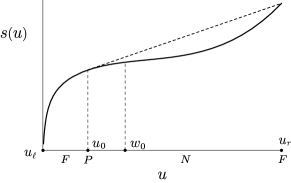
Figure 1: Schematic graph of $s(u)$, showing the set $F=(u_{\ell},u_{0})\cup\{u_{r}\}$ of full ensemble equivalence, the singleton set $P=\{u_{0}\}$ of partial equivalence, and the set $N=(u_{0},u_{r})$ of nonequivalence, where $u_{\ell}=-\frac{1}{2}$ and $u_{r}=-\frac{1}{2q}$. For $u\in F\cup P=(u_{\ell},u_{0}]\cup\{u_{r}\}$, $s(u)=s^{**}(u)$; for $u\in N$, $s(u)<s^{**}(u)$ and the graph of $s^{**}$ consists of the dotted line segment with slope $\beta_{c}$. The slope of $s$ at $u_{\ell}$ is $\infty$. The quantity $w_{0}$ is discussed after Conjecture 5.1.

We define the sets

$$F=(u_{\ell},u_{0})\cup\{u_{r}\},\ P=\{u_{0}\},\ and\ N=(u_{0},u_{r}).$$

Figure 1 and Theorem 3.1 then show that these sets are respectively the sets of full equivalence, partial equivalence, and nonequivalence of the microcanonical and canonical ensembles. The details are given in the next three items. In Theorem 6.2 in CosEllTou1 all these conclusions concerning ensemble equivalence and nonequivalence are proved analytically without reference to the form of $s$ given in Figure 1.

1. $s$ is strictly concave on the interval $(u_{\ell},u_{0})$ and has a strictly supporting line at each $u\in(u_{\ell},u_{0})$ and at $u_{r}$. Hence for $u\in F=(u_{\ell},u_{0})\cup\{u_{r}\}$ the ensembles are fully equivalent in the sense that there exists $\beta$ such that ${\cal E}^{u}={\cal E}_{\beta}$ [Thm. 3.1(a)].

2. $s$ is concave but not strictly concave at $u_{0}$ and has a nonstrictly supporting line at $u_{0}$ that also touches the graph of $s$ over the right hand endpoint $u_{r}$. Hence for $u\in P=\{u_{0}\}$ the ensembles are partially equivalent in the sense that there exists $\beta$ such that ${\cal E}^{u}\subset{\cal E}_{\beta}$ but ${\cal E}^{u}\not={\cal E}_{\beta}$ [Thm. 3.1(b)].

3. $s$ is not concave on $N=(u_{0},u_{r})$ and has no supporting line at any $u\in N$. Hence for $u\in N$ the ensembles are nonequivalent in the sense that for all $\beta$, ${\cal E}^{u}\cap{\cal E}_{\beta}=\emptyset$ [Thm. 3.1(c)].

The explicit calculation of the elements of ${\cal E}_{\beta}$ and ${\cal E}^{u}$ given in CosEllTou1 shows different continuity properties of these two sets. ${\cal E}_{\beta}$ undergoes a discontinuous phase transition as $\beta$ increases through the critical inverse temperature $\beta_{c}=\frac{2(q-1)}{q-2}\log(q-1)$, the unique macrostate $\rho$ for $\beta<\beta_{c}$ bifurcating discontinuously into the $q$ distinct macrostates for $\beta>\beta_{c}$. By contrast, ${\cal E}^{u}$ undergoes a continuous phase transition as $u$ decreases from the maximum value $u_{r}=-\frac{1}{2q}$, the unique macrostate $\rho$ for $u=u_{r}$ bifurcating continuously into the $q$ distinct macrostates for $u<u_{r}$. The different continuity properties of these phase transitions shows already that the canonical and microcanonical ensembles are nonequivalent.

For $u$ in the interval $N$ of ensemble nonequivalence, the graph of $s^{**}$ is affine; this is depicted by the dotted line segment in Figure 1. One can show that the slope of the affine portion of the graph of $s^{**}$ equals the critical inverse temperature $\beta_{c}$.

This completes the discussion of the equivalence and nonequivalence of the microcanonical and canonical ensembles. The equivalence and nonequivalence of the microcanonical and Gaussian ensembles depends on the relationships between the sets ${\cal E}^{u}$ and ${\cal E}_{\beta,\gamma}$ of corresponding equilibrium macrostates, which in turn are determined by support properties of the generalized microcanonical entropy $s_{\gamma}(u)=s(u)-\gamma u^{2}$. As we just saw, for each $u\in N=(u_{0},u_{r})$, the microcanonical and canonical ensembles are nonequivalent. For $u\in N$ we would like to recover equivalence by replacing the canonical ensemble by an appropriate Gaussian ensemble.

Unfortunately, Theorem 4.2 is not applicable. Although the first three of the hypotheses are valid, unfortunately $s^{\prime\prime}$ is not bounded above on the interior of $\mbox{dom}\,s$. Indeed, using the explicit formula for $s$ given in Theorem 4.3 in CosEllTou1 , one verifies that $\lim_{u\rightarrow(u_{r})^{-}}s^{\prime\prime}(u)=\infty$. However, we can appeal to Theorem 4.3, which is applicable since $s$ is twice continuously differentiable on $N$. We conclude that for each $u\in N$ and all sufficiently large $\gamma$ there exists a corresponding Gaussian ensemble that is equivalent to the microcanonical ensemble for that $u$.

By using other conjectured properties of the microcanonical entropy, we are able to deduce the stronger result on the equivalence of the microcanonical and Gaussian ensembles stated in Theorem 5.2. As before, we denote $\mbox{dom}\,s$ by $[u_{\ell},u_{r}]$, where $u_{\ell}=-\frac{1}{2}$ and $u_{r}=-\frac{1}{2q}$, and write

$$s^{\prime}(u_{\ell})=\lim_{u\rightarrow(u_{\ell})^{+}}s^{\prime}(u)\ \mbox{ and }\ s^{\prime}(u_{r})=\lim_{u\rightarrow(u_{r})^{-}}s^{\prime}(u)$$

with a similar notation for $s^{\prime\prime}(u_{\ell})$ and $s^{\prime\prime}(u_{r})$. Using the explicit but complicated formula for $s$ given in Theorem 4.2 in CosEllTou1 , the following conjecture was verified numerically for all $q\in\{4,5,\ldots,10^{4}\}$ and all $u\in(u_{\ell},u_{r})$ of the form $u=u_{\ell}+0.02k$, where $k$ is a positive integer.

Conjecture 5.1.

For all $q\geq 3$ the microcanonical entropy $s$ has the following two properties.

(a) $s^{\prime\prime\prime}(u)>0$ for all $u\in(u_{\ell},u_{r})$.

(b) $s^{\prime}(u_{\ell})=\infty,\ 0<s^{\prime}(u_{r})<\infty,\ s^{\prime\prime}(u_{\ell})=-\infty,\ \mbox{ and }\ s^{\prime\prime}(u_{r})=\infty$.

The conjecture implies that $s^{\prime\prime}$ is an increasing bijection of $(u_{\ell},u_{r})$ onto ${\mathbb{R}}$. Therefore, there exists a unique point $w_{0}\in(u_{\ell},u_{r})$ such that $s^{\prime\prime}(u)<0$ for all $u\in(u_{\ell},w_{0})$, $s^{\prime\prime}(w_{0})=0$, and $s^{\prime\prime}(u)>0$ for all $u\in(w_{0},u_{r})$. It follows that the restriction of $s$ to $[u_{\ell},w_{0}]$ is strictly concave and the restriction of $s$ to $[w_{0},u_{r}]$ is strictly convex. These properties, which can be seen in Figure 1, are summarized by saying that $s$ is a concave-convex function with break point $w_{0}$.

The interval $N=(u_{0},u_{r})$ exhibited in Figure 1 contains all energy values $u$ for which there exists no canonical ensemble that is equivalent with the microcanonical ensemble. Assuming the truth of Conjecture 5.1, we now show that for each $u\in N$ there exists $\gamma\geq 0$ and an associated Gaussian ensemble that is equivalent with the microcanonical ensemble for all $v\leq u$. In order to do this, for $\gamma\geq 0$ we bring in the generalized microcanonical entropy

$$s_{\gamma}(u)=s(u)-\gamma u^{2}$$

and note that the properties of $s$ stated in Conjecture 5.1 are invariant under the addition of the quadratic $-\gamma u^{2}$. Hence, if Conjecture 5.1 is valid, then $s_{\gamma}$ satisfies the same properties as $s$. In particular, $s_{\gamma}$ must be a concave-convex function with some break point $w_{\gamma}$, which is the unique point in $(u_{\ell},u_{r})$ such that $s_{\gamma}^{\prime\prime}(u)<0$ for all $u\in(u_{\ell},w_{\gamma})$, $s_{\gamma}^{\prime\prime}(w_{\gamma})=0$, and $s_{\gamma}^{\prime\prime}(u)>0$ for all $u\in(w_{\gamma},u_{r})$. A straightforward argument, which we omit, and an appeal to Theorem 3.3 show that there exists a unique point $u_{\gamma}\in(u_{\ell},w_{\gamma})$ having the properties listed in the next three items. These properties show that $u_{\gamma}$ plays the same role for ensemble equivalence involving the Gaussian ensemble that the point $u_{0}$ plays for ensemble equivalence involving the canonical ensemble.

1. For $\gamma\geq 0$, $s_{\gamma}$ is strictly concave on the interval $(u_{\ell},u_{\gamma})$ and has a strictly supporting line at each $u\in(u_{\ell},u_{\gamma})$ and at $u_{r}$. Hence for $u\in F_{\gamma}=(u_{\ell},u_{\gamma})\cup\{u_{r}\}$ the ensembles are fully equivalent in the sense that there exists $\beta$ such that ${\cal E}^{u}={\cal E}_{\beta,\gamma}$ [Thm. 3.3(a)].

2. For $\gamma\geq 0$, $s_{\gamma}$ is concave but not strictly concave at $u_{\gamma}$ and has a nonstrictly supporting line at $u_{\gamma}$ that also touches the graph of $s$ over the right hand endpoint $u_{r}$. Hence for $u\in P_{\gamma}=\{u_{\gamma}\}$ the ensembles are partially equivalent in the sense that there exists $\beta$ such that ${\cal E}^{u}\subset{\cal E}_{\beta,\gamma}$ but ${\cal E}^{u}\not={\cal E}_{\beta,\gamma}$ [Thm. 3.3(b)].

3. For $\gamma\geq 0$, $s_{\gamma}$ is not concave on the interval $N=(u_{\gamma},u_{r})$ and has no supporting line at any $u\in N$. Hence for $u\in N_{\gamma}$ the ensembles are nonequivalent in the sense that for all $\beta$, ${\cal E}^{u}\cap{\cal E}_{\beta,\gamma}=\emptyset$ [Thm. 3.3(c)].

We now state our main result.

Theorem 5.2.

We assume that Conjecture 5.1 is valid. Then as a function of $\gamma\geq 0$, $F_{\gamma}=(u_{\ell},u_{\gamma})\cup\{u_{r}\}$ is strictly increasing, and as $\gamma\rightarrow\infty$, $F_{\gamma}\uparrow(u_{\ell},u_{r}]$. It follows that for any $u\in N=(u_{0},u_{r})$, there exists $\gamma\geq 0$ such that the microcanonical ensemble and the Gaussian ensemble defined in terms of this $\gamma$ are fully equivalent for all $v\in(u_{\ell},u_{r})$ satisfying $v\leq u$. The value of $\beta$ defining the Gaussian ensemble is unique and is given by $\beta=s^{\prime}(v)-2\gamma v$.

The proof of the theorem relies on the next lemma, part (a) of which uses Proposition 4.1. When applied to $s_{\gamma}$, this proposition states that $s_{\gamma}$ has a strictly supporting line at a point if and only if $s$ has a strictly supporting parabola at that point. Proposition 4.1 illustrates why one can achieve full equivalence with the Gaussian ensemble when full equivalence with the canonical ensemble fails. Namely, even when $s$ does not have a supporting line at a point, it might have a supporting parabola at that point; in this case the supporting parabola can be made strictly supporting by increasing $\gamma$. The proofs of parts (b)–(d) of the next lemma rely on Theorem 4.3 and on the properties of the sets $F_{\gamma}$, $P_{\gamma}$, and $N_{\gamma}$ stated in the three items appearing just before the last theorem.

Lemma 5.3.

We assume that Conjecture 5.1 is valid. Then the following conclusions hold.

(a) If for some $\gamma\geq 0$, $s_{\gamma}$ has a supporting line at a point $u$, then for any $\tilde{\gamma}>\gamma$, $s_{\tilde{\gamma}}$ has a strictly supporting line at $u$.

(b) For any $0\leq\gamma<\tilde{\gamma}$, $F_{\gamma}\cup P_{\gamma}\subset F_{\tilde{\gamma}}$.

(c) $u_{\gamma}$ is a strictly increasing function of $\gamma\geq 0$ and $\lim_{\gamma\rightarrow\infty}u_{\gamma}=u_{r}$.

(d) As a function of $\gamma\geq 0$, $F_{\gamma}$ is strictly increasing.

Proof. (a) Suppose that $s_{\gamma}$ has a supporting line at $u$ with slope $\bar{\beta}$. Then by Proposition 4.1 $s$ has a supporting parabola at $u$ with parameters $(\beta,\gamma)$, where $\beta=\bar{\beta}+2\gamma u$. As the definition (4.1) makes clear, replacing $\gamma$ by any $\tilde{\gamma}>\gamma$ makes the supporting parabola at $u$ strictly supporting. Again by Proposition 4.1 $s_{\tilde{\gamma}}$ has a strictly supporting line at $u$.

(b) If $u\in F_{\gamma}\cup P_{\gamma}$, then $s_{\gamma}$ has a supporting line at $u$. Since $0\leq\gamma<\tilde{\gamma}$, part (a) implies that $s_{\tilde{\gamma}}$ has a strictly supporting line at $u$. Hence $u$ must be an element of $F_{\tilde{\gamma}}$.

(c) If $0\leq\gamma<\tilde{\gamma}$, then by part (a) of the present lemma $u_{\gamma}\in P_{\gamma}\subset F_{\tilde{\gamma}}$. Since $F_{\tilde{\gamma}}=(u_{\ell},u_{\tilde{\gamma}})\cup\{u_{r}\}$ and since $u_{\gamma}<u_{r}$, it follows that $u_{\gamma}<u_{\tilde{\gamma}}$. Thus $u_{\gamma}$ is a strictly increasing function of $\gamma\geq 0$. We now prove that $\lim_{\gamma\rightarrow\infty}u_{\gamma}=u_{r}$. For any $u\in(u_{\ell},u_{r})$, part (b) of Theorem 4.3 states that there exists $\gamma_{u}>0$ such that $s_{\gamma_{u}}(u)$ has a strictly supporting line at $u$. It follows that $u\in F_{\gamma_{u}}=(u_{\ell},u_{\gamma_{u}})\cup\{u_{r}\}$ and thus that $u<u_{\gamma_{u}}<u_{r}$. Since $u_{\gamma}$ is a strictly increasing function of $\gamma$, it follows that for all $\gamma>\gamma_{u}$, we have $u_{\gamma}>u_{\gamma_{u}}>u$. We have shown that for any $u\in(u_{\ell},u_{r})$, there exists $\gamma_{u}>0$ such that for all $\gamma>\gamma_{u}$, we have $u_{\gamma}>u$. This completes the proof that $\lim_{\gamma\rightarrow\infty}u_{\gamma}=u_{r}$.

(d) Since $F_{\gamma}=(u_{\ell},u_{\gamma})\cup\{u_{r}\}$, this follows immediately from the first property of $u_{\gamma}$ in part (c). The proof of the lemma is complete.   

We are now ready to prove Theorem 5.2. The properties of $F_{\gamma}$ stated there follow immediately from Lemma 5.3. Indeed, since $u_{\gamma}$ is a strictly increasing function of $\gamma\geq 0$, $F_{\gamma}$ is also strictly increasing. In addition, since $\lim_{\gamma\rightarrow\infty}u_{\gamma}=u_{r}$ it follows that as $\gamma\rightarrow\infty$, $F_{\gamma}\uparrow(u_{\ell},u_{r}]$. Since $F_{\gamma}$ is the set of full ensemble equivalence, we conclude that for any $u\in N=(u_{0},u_{r})$, there exists $\gamma>0$ such that the microcanonical ensemble and the Gaussian ensemble defined in terms of this $\gamma$ are fully equivalent for all $v\in(u_{\ell},u_{r})$ satisfying $v\leq u$. The last statement concerning $\beta$ is a consequence of part (c) of Theorem 4.3. The proof of Theorem 5.2 is complete.

- (1) J. Barré, D. Mukamel, and S. Ruffo. Ensemble inequivalence in mean-field models of magnetism. T. Dauxois, S. Ruffo, E. Arimondo, M. Wilkens (editors). Dynamics and Thermodynamics of Systems with Long Interactions, pp. 45–67. Volume 602 of Lecture Notes in Physics. New York: Springer-Verlag, 2002.
- (2) J. Barré, D. Mukamel, and S. Ruffo. Inequivalence of ensembles in a system with long-range interactions. Phys. Rev. Lett. 87:030601, 2001.
- (3) D. P. Bertsekas. Constrained Optimization and Lagrange Multiplier Methods. New York: Academic Press, 1982.
- (4) M. Blume, V. J. Emery, and R. B. Griffiths. Ising model for the transition and phase separation in - mixtures. Phys. Rev. A 4:1071–1077, 1971.
- (5) E. P. Borges and C. Tsallis. Negative specific heat in a Lennard-Jones-like gas with long-range interactions. Physica A 305:148–151, 2002.
- (6) C. Boucher, R. S. Ellis, and B. Turkington. Derivation of maximum entropy principles in two-dimensional turbulence via large deviations. J. Statist. Phys. 98:1235–1278, 2000.
- (7) E. Caglioti, P. L. Lions, C. Marchioro, and M. Pulvirenti. A special class of stationary flows for two-dimensional Euler equations: a statistical mechanical description. Commun. Math. Phys. 143:501–525, 1992.
- (8) M. S. S. Challa and J. H. Hetherington. Gaussian ensemble: an alternate Monte-Carlo scheme. Phys. Rev. A 38:6324–6337, 1988.
- (9) M. S. S. Challa and J. H. Hetherington. Gaussian ensemble as an interpolating ensemble. Phys. Rev. Lett. 60:77–80, 1988.
- (10) M. Costeniuc, R. S. Ellis, and H. Touchette. Complete analysis of phase transitions and ensemble equivalence for the Curie-Weiss-Potts model. J. Math. Phys. 46:063301, 2005
- (11) M. Costeniuc, R. S. Ellis, and H. Touchette. Nonconcave entropies from generalized canonical ensembles. Submitted to Phys. Rev. Lett., 2006. LANL reprint cond-mat/0605213.
- (12) M. Costeniuc, R. S. Ellis, H. Touchette, and B. Turkington. The generalized canonical ensemble and its universal equivalence with the microcanonical ensemble. J. Stat. Phys. 119:1283–1329, 2005.
- (13) M. Costeniuc, R. S. Ellis, H. Touchette, and B. Turkington. Generalized canonical ensembles and ensemble equivalence. Phys. Rev. E 73:026105, 2006.
- (14) T. Dauxois, V. Latora, A. Rapisarda, S. Ruffo, and A. Torcini. The Hamiltonian mean field model: from dynamics to statistical mechanics and back. In T. Dauxois, S. Ruffo, E. Arimondo, and M. Wilkens, editors, Dynamics and Thermodynamics of Systems with Long-Range Interactions, volume 602 of Lecture Notes in Physics, pages 458–487, New York, 2002. Springer-Verlag.
- (15) T. Dauxois, P. Holdsworth, and S. Ruffo. Violation of ensemble equivalence in the antiferromagnetic mean-field XY model. Eur. Phys. J. B 16:659, 2000.
- (16) J.-D. Deuschel, D. W. Stroock, and H. Zessin. Microcanonical distributions for lattice gases. Commun. Math. Phys. 139:83–101, 1991.
- (17) M. DiBattista, A. Majda, and M. Grote. Meta-stability of equilibrium statistical structures for prototype geophysical flows with damping and driving. Physica D 151:271–304, 2000.
- (18) M. DiBattista, A. Majda, and B. Turkington. Prototype geophysical vortex structures via large-scale statistical theory. Geophys. Astrophys. Fluid Dyn. 89:235–283, 1998.
- (19) R. S. Ellis. Entropy, Large Deviations, and Statistical Mechanics. New York: Springer-Verlag, 1985. Reprinted in Classics in Mathematics, 2006.
- (20) R. S. Ellis, K. Haven, and B. Turkington. Analysis of statistical equilibrium models of geostrophic turbulence. J. Appl. Math. Stoch. Anal. 15:341–361, 2002.
- (21) R. S. Ellis, K. Haven, and B. Turkington. Large deviation principles and complete equivalence and nonequivalence results for pure and mixed ensembles. J. Statist. Phys. 101:999–1064 , 2000.
- (22) R. S. Ellis, K. Haven, and B. Turkington. Nonequivalent statistical equilibrium ensembles and refined stability theorems for most probable flows. Nonlinearity 15:239–255, 2002.
- (23) R. S. Ellis, R. Jordan, P. Otto, and B. Turkington. A statistical approach to the asymptotic behavior of a generalized class of nonlinear Schrödinger equations. Commun. Math. Phys. 244:187–208, 2004.
- (24) R. S. Ellis, P. Otto, and H. Touchette. Analysis of phase transitions in the mean-field Blume-Emery-Griffiths model. Ann. Appl. Prob. 15:2203 –2254, 2004.
- (25) R. S. Ellis, H. Touchette, and B. Turkington. Thermodynamic versus statistical nonequivalence of ensembles for the mean-field Blume-Emery-Griffith model. Physica A 335:518 –538, 2004.
- (26) G. L. Eyink and H. Spohn. Negative-temperature states and large-scale, long-lived vortices in two-dimensional turbulence. J. Statist. Phys. 70:833–886, 1993.
- (27) H. Föllmer and S. Orey, Large deviations for the empirical field of a Gibbs measure. Ann. Prob. 16:961–977, 1987.
- (28) H.-O. Georgii. Large deviations and maximum entropy principle for interacting random fields on . Ann. Probab. 21:1845–1875, 1993.
- (29) J. W. Gibbs. Elementary Principles in Statistical Mechanics with Especial Reference to the Rational Foundation of Thermodynamics. Yale University Press, New Haven, 1902. Reprinted by Dover, New York, 1960.
- (30) D. H. E. Gross. Microcanonical thermodynamics and statistical fragmentation of dissipative systems: the topological structure of the -body phase space. Phys. Rep. 279:119–202, 1997.
- (31) P. Hertel and W. Thirring. A soluble model for a system with negative specific heat. Ann. Phys. (NY) 63:520, 1971.
- (32) J. H. Hetherington. Solid 3He magnetism in the classical approximation. J. Low Temp. Phys. 66:145–154, 1987.
- (33) J. H. Hetherington and D. R. Stump. Sampling a Gaussian energy distribution to study phase transitions of the Z(2) and U(1) lattice gauge theories. Phys. Rev. D 35:1972–1978, 1987.
- (34) R. S. Johal, A. Planes, and E. Vives. Statistical mechanics in the extended Gaussian ensemble. Phys. Rev. E 68:056113, 2003.
- (35) R. Jordan, B. Turkington, and C. L. Zirbel A mean-field statistical theory for the nonlinear Schrödinger equation. Physica D 137:353–378, 2000.
- (36) M. K.-H. Kiessling and J. L. Lebowitz. The micro-canonical point vortex ensemble: beyond equivalence. Lett. Math. Phys. 42:43–56, 1997.
- (37) M. K.-H. Kiessling and T. Neukirch. Negative specific heat of a magnetically self-confined plasma torus. Proc. Natl. Acad. Sci. USA 100:1510–1514, 2003.
- (38) O. E. Lanford. Entropy and equilibrium states in classical statistical mechanics. In Statistical Mechanics and Mathematical Problems: Battelle Seattle 1971 Rencontres, ed. A. Lenard, 1–113. Lecture Notes in Physics, Vol. 20. Springer-Verlag, Berlin, 1973.
- (39) V. Latora, A. Rapisarda, and C. Tsallis. Non-Gaussian equilibrium in a long-range Hamiltonian system. Phys. Rev. E 64:056134, 2001.
- (40) J. L. Lebowitz, H. A. Rose, and E. R. Speer. Statistical mechanics of a nonlinear Schrödinger equation. II. Mean field approximation. J. Statist. Phys. 54:17–56, 1989.
- (41) J. T. Lewis, C.-E. Pfister, and W. G. Sullivan. The equivalence of ensembles for lattice systems: some examples and a counterexample. J. Statist. Phys. 77:397–419, 1994.
- (42) J. T. Lewis, C.-E. Pfister, and W. G. Sullivan. Entropy, concentration of probability and conditional limit theorems. Markov Proc. Related Fields 1:319–386, 1995.
- (43) D. Lynden-Bell and R. Wood. The gravo-thermal catastrophe in isothermal spheres and the onset of red-giant structure for stellar systems. Mon. Notic. Roy. Astron. Soc. 138:495, 1968.
- (44) J. Miller. Statistical mechanics of Euler equations in two dimensions. Phys. Rev. Lett. 65:2137–2140, 1990.
- (45) M. Minoux. Mathematical Programming: Theory and Algorithms. Chichester: Wiley-Interscience, John-Wiley and Sons, 1986.
- (46) S. Olla. Large deviations for Gibbs random fields. Probab. Th. Rel. Fields 77:343–359, 1988.
- (47) R. Robert. A maximum-entropy principle for two-dimensional perfect fluid dynamics. J. Statist. Phys. 65:531–553, 1991.
- (48) R. Robert and J. Sommeria. Statistical equilibrium states for two-dimensional flows. J. Fluid Mech. 229:291–310, 1991.
- (49) R. T. Rockafellar. Convex Analysis. Princeton, NJ: Princeton University Press, 1970.
- (50) S. Roelly and H. Zessin. The equivalence of equilibrium principles in statistical mechanics and some applications to large particle systems. Expositiones Mathematicae 11:384–405, 1993.
- (51) R. A. Smith and T. M. O’Neil. Nonaxisymmetric thermal equilibria of a cylindrically bounded guiding center plasma or discrete vortex system. Phys. Fluids B 2:2961–2975, 1990.
- (52) D. R. Stump and J. H. Hetherington. Remarks on the use of a microcanonical ensemble to study phase transitions in the lattice gauge theory. Phys. Lett. B 188:359–363, 1987.
- (53) W. Thirring. Systems with negative specific heat. Z. Physik 235:339–352, 1970.
- (54) H. Touchette, M. Costeniuc, R. S. Ellis, and B. Turkington. Metastability within the generalized canonical ensemble. Physica A 365:132–137, 2006.
- (55) H. Touchette, R. S. Ellis, and B. Turkington. An introduction to the thermodynamic and macrostate levels of nonequivalent ensembles. Physica A 340:138–146, 2004.
- (56) B. Turkington, A. Majda, K. Haven, and M. DiBattista. Statistical equilibrium predictions of jets and spots on Jupiter. Proc. Natl. Acad. Sci. USA 98:12346–12350, 2001.
- (57) F. Y. Wu. The Potts model. Rev. Mod. Phys. 54:235–268, 1982.