An Analytic Equation of State for Ising-like Models

Abstract

Using an Environmentally Friendly Renormalization we derive, from an underlying field theory representation, a formal expression for the equation of state, $y=f(x)$, that exhibits all desired asymptotic and analyticity properties in the three limits $x\rightarrow 0$, $x\rightarrow\infty$ and $x\rightarrow-1$. The only necessary inputs are the Wilson functions $\gamma_{\lambda}$, $\gamma_{\varphi}$ and $\gamma_{\varphi^{2}}$, associated with a renormalization of the transverse vertex functions. These Wilson functions exhibit a crossover between the Wilson-Fisher fixed point and the fixed point that controls the coexistence curve. Restricting to the case $N=1$, we derive a one-loop equation of state for $2<d<4$ naturally parameterized by a ratio of non-linear scaling fields. For $d=3$ we show that a non-parameterized analytic form can be deduced. Various asymptotic amplitudes are calculated directly from the equation of state in all three asymptotic limits of interest and comparison made with known results. By positing a scaling form for the equation of state inspired by the one-loop result, but adjusted to fit the known values of the critical exponents, we obtain better agreement with known asymptotic amplitudes.

I Introduction

The universal equation of state for the Landau-Ginzburg-Wilson $O(N)$ model remains a subject of great interest (see, for instance, zinnjustin and Pelisseto for recent reviews). Its calculation from first principles is much more difficult than the calculation of other universal quantities, such as critical exponents or amplitude ratios. The universal equation of state for the scaling function exhibits crossover behavior between three distinct, asymptotic regimes - the critical region when approached from the critical isotherm, or when approached along the critical isochor, and the coexistence curve. Maintaining the correct analyticity properties of the equation of state in all these three distinct regimes has not been possible within the confines of first principle calculations, such as from a field-theoretic, microscopic Hamiltonian. Rather, appeal has been made to a parameterized phenomenological scaling ansatz Schofield that exhibits the right asymptotics, the underlying microscopic theory then being used to fix various free parameters that exist in the ansatz.

In this paper we use a renormalization group methodology - Environmentally Friendly Renormalization Stephens - based only on an underlying Landau-Ginzburg-Wilson Hamiltonian and without the need for any phenomenological ansatz, to derive an equation of state that exhibits all desired analyticity properties in the three distinct asymptotic regimes.

II The Equation of State

As first noted by Widom Widom , in the critical region, the equation of state is a homogeneous function relating an external magnetic field $H$, the reduced temperature $t$, and the magnetization $\varphi$, which can be expressed by

$$y=f\left(x\right)$$ (1)

where $f(x)$ is universal, the scaling variables $y$ and $x$ are $y=B_{c}^{\delta}H/\varphi^{\delta}$ and $x=B^{1/\beta}t/\varphi^{1/\beta}$, and $B_{c}$ and $B$ are non-universal amplitudes associated with the behavior on the critical isotherm $t=0$ and the coexistence curve $t<0$, $H=0$.

The scaling function $f(x)$ is normalized such that $f(0)=1$ on the critical isotherm, and $f(-1)=0$ on the coexistence curve. Several properties of the universal equation of state are known rigorously. For instance, it is known that $f(x)$ has a regular Taylor expansion around the limit $x=0$ given by

$$f(x)=1+\sum_{n=1}^{\infty}f^{0}_{n}x^{n},$$ (2)

while in the limit $x\rightarrow\infty$, by Griffith’s analyticity, one has an expansion of the form

$$f(x)=x^{\gamma}\sum_{n=0}^{\infty}f^{\infty}_{n}x^{-2n\beta}$$ (3)

In the limit $x\rightarrow\infty$ a natural variable is $z=b_{1}\varphi/t^{\beta}$, where $b_{1}={(-C_{4}^{+}/{(C^{+})}^{3})}^{1/2}$ and the $C_{2n}^{+}$ are the amplitudes of the $2n$-point correlation functions for $T>T_{c}$, $C^{+}$ being the amplitude of the susceptibility. In terms of $z$ the equation of state takes the form

$$H=-(-C^{+}/C_{4}^{+})^{1/2}t^{\beta\delta}F(z)$$ (4)

where the universal scaling function $F(z)$ for small $z$ has an expansion of the form

$$F(z)=z+\frac{1}{6}z^{3}+\sum_{n=3}^{\infty}\frac{r_{2n}}{(2n-1)!}z^{2n-1}$$ (5)

where $r_{2}=r_{4}=1$ by choice of normalization. As (5) is an expansion in $\varphi$, the constants $r_{2n}$ are related to the $2n$-point correlation functions at $\varphi=0$ and hence are very natural observables to calculate in lattice simulations. In the limit $z\rightarrow\infty$, $F(z)$ has an expansion of the form

$$F(z)=z^{\delta}\sum_{k=0}^{\infty}F_{k}^{\infty}z^{-k/\beta}$$ (6)

The universal scaling functions $f(x)$ and $F(z)$ are related via

$$z^{-\delta}F(z)=F_{0}^{\infty}f(x)$$ (7)

with $z=z_{0}x^{-\beta}$, where $z_{0}$ is the universal zero of the equation of state in terms of the variable $z$. Hence, the expansion coefficients of the two functions can be related to find

$$f_{n}^{\infty} = z_{0}^{2n+1-\delta}\frac{r_{2n+2}}{F_{0}^{\infty}(2n+1)!}$$ (8)

$$f_{n}^{0} = \frac{F_{n}^{\infty}}{F_{0}^{\infty}}z_{0}^{-n/\beta}$$ (9)

Thus, we see it is sufficient to know the expansion coefficients of $f(x)$ in the limits $x\rightarrow 0$ and $\infty$ in order to calculate the asymptotic properties of $F(z)$ and the interesting coefficients $r_{2n}$.

Unlike the limits $x\rightarrow 0$ and $\infty$, near the coexistence curve, $x\rightarrow-1$, there are no rigorous mathematical arguments as to the analyticity properties of $f(x)$, although there do exist conjectures. For instance, for $N>1$ in Wallace , based on an $\varepsilon$-expansion analysis, it was conjectured that $(1+x)$ has a double expansion in powers of $y$ and $y^{(d-2)/2}$ of the form

$$1+x=c_{1}y+c_{2}y^{1-\epsilon/2}+d_{1}y^{2}+d_{2}y^{2-\epsilon/2}+...$$ (10)

In three dimensions it predicts an expansion of $(1+x)$ in powers of $y^{1/2}$.

Of course, the behavior in the vicinity of the coexistence curve depends on the value of $N$. For $N=1$, the longitudinal correlation length remains finite away from the critical point on the coexistence curve, while for $N>1$, the existence of Goldstone bosons leads to infrared singularities. For $N=1$, one may formally posit that in the vicinity of the coexistence curve

$$f(x)=\sum_{n=1}^{\infty}f_{n}^{c}(1+x)^{n}$$ (11)

the integer powers being a reflection of the finite longitudinal correlation length. For Ising-like systems essential singularities are to be expected. Of course, these cannot be captured within the confines of an ansatz like (11). For $N>1$ studies of the non-linear $\sigma$ model lead one to expect a leading behavior of the form

$$f(x)\sim c_{f}(1+x)^{2/(d-2)}$$ (12)

though, as mentioned, the nature of the corrections to this behavior is not well understood, although (10) is one conjecture. In the $1/N$ expansion there is some evidence Pelisseto for logarithmic corrections of the form $\ln(1+x)$ in three dimensions.

Early field theoretic calculations using the renormalization group with an $\varepsilon$-expansion Brezin foundered on the fact that they did not exhibit Griffiths analyticity in the large $x$ limit. Irrespective of the expansion method - $\varepsilon$-, fixed-dimension, $1/N$ etc. - there will remain a fundamental difficulty - that an expansion around a particular fixed point will not readily access the universal equation of state in the entire phase diagram, due to the presence of other fixed points that must be accessed. Simply put, the equation of state exhibits crossovers, and the nature of these crossovers depends on $N$. For $N=1$ the theory is controlled by a “Gaussian” or mean-field fixed point, wherein fluctuations are suppressed on the coexistence curve away from the critical point by the non-vanishing longitudinal mass. In distinction, for $N>1$, the theory is dominated by the massless Goldstone excitations on the coexistence curve and the non-linear $\sigma$ model gives a good description Lawrie .

The problem of incorporating Griffiths analyticity was solved by using a parameterized formulation in terms of new variables $R$ and $\theta$, related to $t$ and $\varphi$ via

$$\varphi=m_{0}R^{\beta}m(\theta)$$

$$t=R(1-\theta^{2})$$

$$H=h_{0}R^{\beta\delta}h(\theta)$$

where the two functions $m(\theta)$ and $h(\theta)$ are undetermined. In this new parameterization the scaling variable $x$ and the scaling function $f(x)$ are given by

$$x = \frac{1-\theta^{2}}{\theta_{0}^{2}-1}\left(\frac{m\left(\theta_{0}\right)}{m\left(\theta\right)}\right)^{1/\beta}$$ (13)

$$f\left(x\right) = \left(\frac{m\left(\theta\right)}{m\left(1\right)}\right)^{-\delta}\frac{h\left(\theta\right)}{h\left(1\right)}$$ (14)

Most current field theoretic formulations for determining the equation of state (see zinnjustin ; Pelisseto for comprehensive reviews) rely on such formulations. The drawback is that the underlying microscopic theory is not used to determine the functional form of $m(\theta)$ and $h(\theta)$, rather an ansatz is made as to the general functional form which depends on certain unknown parameters and then the underlying microscopic theory is used to fix these parameters. The most common ansatz is that the functions are polynomials in $\theta$. The coefficients of the powers of $\theta$ are then determined by calculating certain observables independently from the underlying microscopic theory and then using the values of these observables to determine the coefficients. Various methodologies have been used Pelisseto ; Engels ; zinnjustin using a variety of methods. For instance, an expansion of the effective potential for small $\varphi$ for $t>0$ using $\epsilon$ or fixed dimension expansions. Results from Monte-Carlo simulations or high temperature expansions have also been used.

In this paper we apply a new method to describe the equation of state in a uniform manner. Using environmentally friendly renormalizationStephens , we find a schema able to capture the crossover between the Wilson-Fisher fixed point and the fixed point that controls the coexistence curve. By integrating along curves of constant magnetization, we obtain the equation of state in the whole critical region. Moreover, the equation of state that we obtain is parameterized in terms of the inverse of the transverse correlation length, a quantity well defined over the entire phase diagram. The representation we have found is valid for both large and small values of the scaling variables and satisfies Griffiths analyticity. Although our approach works for any $N$ we here concentrate on the case $N=1$.

III A Renormalization Group Representation of the Equation of State

In this section we briefly outline the derivation of the equation of state for a theory described by the standard LGW Hamiltonian with $O(N)$ symmetry

$${\cal H}[{\bf\varphi}]=\int\!d^{d}x\left({1\over 2}\nabla\varphi^{a}\nabla\varphi^{a}\!+{1\over 2}r(x)\varphi^{a}\varphi^{a}\!+{\lambda_{B}\over 4!}(\varphi^{a}\varphi^{a})^{2}\!\right).$$ (15)

with $r=r_{c}+t_{B}$, where $r_{c}$ is the value of $r$ at the critical temperature $T_{c}$ and $t_{B}=\Lambda^{2}\ {(T-T_{c})\over T_{c}}$, $\Lambda$ being the microscopic scale. We denote a generic vertex function by $\Gamma^{(N,M)}_{l\dots lt\dots t}$, where the number of $l$ and $t$ subscripts indicates whether a longitudinal or a transverse propagator is to be attached to the vertex at the corresponding point. When all subscripts are either $l$ or $t$ we will use a single $l$ or $t$, for example $\Gamma^{(N,M)}_{t\dots t}$ will be abbreviated $\Gamma^{(N,M)}_{t}$. Furthermore, when there are no $\varphi^{2}$ insertions (i.e. $M=0$) the second index will be left off e.g. $\Gamma^{(N)}$ indicates $\Gamma^{(N,0)}$.

Due to the Ward identities of the model, it is sufficient to know only the $\Gamma^{(N,M)}_{t}$, as all the other vertex functions can be reconstructed from these. The equation of state is

$$H=\Gamma^{(2)}_{t}\varphi$$ (16)

III.1 Renormalization in terms of Non-Linear Scaling Fields

Due to the existence of large fluctuations in the critical regime a renormalization of the microscopic bare parameters of the form

$$t(m,\kappa) = Z_{\varphi^{2}}^{-1}(\kappa)t_{B}(m)$$ (17)

$$\lambda(\kappa) = Z_{\lambda}(\kappa)\lambda_{B}$$ (18)

$$\varphi(\kappa) = Z_{\varphi}^{-1/2}(\kappa)\varphi_{B}$$ (19)

must be imposed, where $\kappa$ is an arbitrary renormalization scale. The renormalized parameters satisfy the differential equations

$$\kappa{dt(\kappa)\over d\kappa} = \gamma_{\varphi^{2}}(\kappa)t(\kappa)$$ (20)

$$\kappa{d\lambda(\kappa)\over d\kappa} = \gamma_{\lambda}(\kappa)\lambda(\kappa)$$ (21)

$$\kappa{d\varphi(\kappa)\over d\kappa} = -{1\over 2}\gamma_{\varphi}(\kappa)\varphi(\kappa)$$ (22)

where the Wilson functions associated with this coordinate transformation are

$$\gamma_{\varphi^{2}}(\kappa) = -\left.{\kappa{d\over d\kappa}\ln Z_{\varphi^{2}}}\right|_{c}$$ (23)

$$\gamma_{\lambda}(\kappa) = \left.{\kappa{d\over d\kappa}\ln Z_{\lambda}}\right|_{c}$$ (24)

$$\gamma_{\varphi}(\kappa) = \left.{\kappa{d\over d\kappa}\ln Z_{\varphi}}\right|_{c}$$ (25)

and the derivative is taken along an appropriately chosen curve in the phase diagram, which we here denote by $c$. Similarly, integration of the renormalization group equation for any multiplicatively renormalizable $\Gamma^{(N,M)}_{t}$ yields

$$\Gamma^{(N,M)}_{t}(t,\lambda,\varphi)=\ \ \ \ \ \ \ \ \ \ \ \ \ \ \ \ \ \ \ \ \ \ \ \ \ \ \ \ \ \ \ \ \$$

$${\rm e}^{\int^{m_{t}}_{\kappa}({N\over 2}\gamma_{\varphi}-M\gamma_{\varphi^{2}}){dx\over x}}\Gamma^{(N,M)}_{t}(t(\kappa),\lambda(\kappa),\varphi(\kappa))$$ (26)

To impose a specific, as opposed to abstract, coordinate transformation between bare and renormalized theory the renormalization constants $Z_{\varphi}$, $Z_{\varphi^{2}}$ and $Z_{\lambda}$ must be fixed. Here, we impose the explicitly magnetization dependent normalization conditions

$$\left.\partial_{p^{2}}\Gamma_{t}^{(2)}(p,t(\kappa,\kappa),\lambda(\kappa),\varphi(\kappa),\kappa)\right|_{p^{2}=0} = 1$$ (27)

$$\Gamma_{t}^{(2,1)}(0,t(\kappa,\kappa),\lambda(\kappa),\varphi(\kappa),\kappa) = 1$$ (28)

$$\Gamma_{t}^{(4)}(0,t(\kappa,\kappa),\lambda(\kappa),\varphi(\kappa),\kappa) = \lambda.$$ (29)

Note that in this case we impose the normalization conditions on the transverse correlation functions. These conditions serve to fix the three $Z$ functions associated with $\varphi_{B}$, $t_{B}$ and $\lambda_{B}$ while the condition

$$\kappa^{2}=\Gamma_{t}^{(2)}(0,t(\kappa,\kappa),\lambda(\kappa),\varphi(\kappa),\kappa),$$ (30)

serves as a gauge fixing condition that relates the sliding renormalization scale $\kappa$ to the physical temperature $t$ and the physical magnetization $\varphi$. Physically, $\kappa$ is a fiducial value of the non-linear scaling field $m_{t}$, which is the inverse transverse correlation length.

Besides $m_{t}$, the other non-linear scaling field we use to parameterize our results is

$$m_{\varphi}^{2}={1\over 3}{\Gamma_{t}^{(4)}\varphi^{2}\over\partial_{p^{2}}\Gamma_{t}^{(2)}|_{p^{2}=0}}$$ (31)

which is an RG invariant. It represents the anisotropy in the masses of the longitudinal and transverse modes and is related to the stiffness constant $\rho_{s}=\varphi^{2}\partial_{p^{2}}\Gamma_{t}^{(2)}|_{p^{2}=0}$ via $m_{\varphi}^{2}={1\over 3}\lambda\rho_{s}$.

With a given renormalization prescription one may determine the equation of state in terms of the non-linear scaling fields $m_{t}$ and $m_{\varphi}$, as the transverse and longitudinal propagators that appear in all perturbative diagrams can be parameterized in terms of them. One of the main motivations for this reparametrization in terms of non-linear scaling fields is that it eliminates all tadpole diagrams at higher loop order. However, what is required is the equation of state in terms of the linear scaling fields $t$ and $\varphi$. One must therefore determine the coordinate transformation, $t=t(m_{t},m_{\varphi})$, $\varphi=\varphi(m_{t},m_{\varphi})$, between them.

III.2 Relating Non-linear and Linear Scaling Fields

This may be done by specifying a particular curve, $c$, in the phase diagram along which we integrate the differential relation for the tranverse vertex functions $\Gamma^{(N)}_{t}$. For example,

$$d\Gamma^{(2)}_{t}=\Gamma^{(2,1)}_{t}dt+{1\over 6}\Gamma^{(4)}_{t}d\varphi^{2}$$ (32)

can be integrated along a curve of constant $\varphi$ to yield $dt=d\Gamma^{(2)}_{t}/\Gamma^{(2,1)}_{t}$, where the right hand side is naturally written in the coordinate system $(m_{t},m_{\varphi})$. To integrate the renormalization group equation for the vertex functions it is most natural to use $m_{t}=\kappa$ as the flow variable and hold $m_{\varphi}$ constant. However, if we then wish to integrate (32) along a curve of constant $\varphi$ we must include a Jacobian factor, $2/(2-\gamma_{\lambda}+\gamma_{\varphi})$, that takes into account the variation of $m_{\varphi}$ along a constant $\varphi$ curve. The relation between $m_{\varphi}$ and $\varphi$ is specified by (31) using the renormalization group equations for $\partial_{p^{2}}\Gamma_{t}^{(2)}$ and $\Gamma_{t}^{(4)}$ with the normalization conditions (27) and (29). Using (III.1) for $\Gamma_{t}^{(2)}$ and $\Gamma_{t}^{(2,1)}$ and the normalization conditions (28) and (30) one may write

$$\frac{d\Gamma^{(2)}_{t}}{\Gamma^{(2,1)}_{t}}=(2-\gamma_{\varphi}){\rm e}^{-\int^{\kappa}_{\kappa_{0}}\gamma_{\varphi^{2}}\frac{dx}{x}}\kappa d\kappa$$ (33)

In the universal limit, where $\lambda\rightarrow\infty$, the crossover to mean field theory is pushed off to infinity and the theory is then controlled in the limit $\kappa\rightarrow\infty$ by the Wilson-Fisher fixed point. Hence, $\gamma_{i}\rightarrow\gamma_{i}^{\rm WF}$, where $\gamma_{i}^{\rm WF}$ is the Wilson function $\gamma_{i}$ at the Wilson-Fisher fixed point. Defining $\Delta\gamma_{i}=(\gamma_{i}-\gamma_{i}^{\rm WF})$ (33) yields

$$dt=(2-\gamma_{\varphi}){\rm e}^{-\int^{\kappa}_{\kappa_{0}}\Delta\gamma_{\varphi^{2}}\frac{dx}{x}}\left({\kappa\over\kappa_{0}}\right)^{-\gamma_{\varphi^{2}}}\kappa d\kappa$$ (34)

To integrate (34) we need to fix some boundary condition. The coexistence curve, where $m_{t}=0$, is a natural one. In this case, $dt$ integrates to the temperature variable $(T-T_{c}(\varphi))$, where $T_{c}(\varphi)$ corresponds to that point on the coexistence curve where the magnetization is $\varphi$. As we wish to use as temperature variable $t=(T-T_{c})$, we may write $(T-T_{c}(\varphi))=t+\Delta$, where $\Delta=(T_{c}-T_{c}(\varphi))$ is the temperature shift that measures the distance between the critical point and the point on the coexistence curve, $T_{c}(\varphi)$. In the integral, $-\int^{\kappa}_{\kappa_{0}}\Delta\gamma_{\varphi^{2}}dx/x$, one may safely take the universal limit, $\kappa_{0}\rightarrow\infty$. In this universal scaling limit, in terms of the linear scaling fields $t$ and $\varphi$, the problem has only one scaling variable, $x$. In terms of the coordinates $m_{t}$ and $m_{\varphi}$, this manifests itself as a reduction to the single scaling variable, $z=m_{t}/m_{\varphi}$. Passing to this variable, using (31), and integrating this along a curve of constant $\varphi$ (taking into account the Jacobian factor) one finds

$$A_{1}(1+x) = \mathcal{F}(z)$$ (35)

where the scaling variable $x=B^{1/\beta}t/\varphi^{1/\beta}$, $B$ being the non-universal amplitude introduced previously, and the universal scaling function $\mathcal{F}(z)$ is

$$\mathcal{F}(z)=\int_{0}^{z}\frac{2(2-\gamma_{\varphi})}{2-\gamma_{\lambda}+\gamma_{\varphi}}D(x)x^{1\over\beta}\frac{dx}{x}$$

where

$$D(x)=\exp\left({-\int_{\infty}^{x}2\left({\frac{\Delta\gamma_{\varphi^{2}}-\frac{\Delta\gamma_{\lambda}}{2\beta}+\frac{\Delta\gamma_{\varphi}}{2\beta}}{2-\gamma_{\lambda}+\gamma_{\varphi}}}\right)\frac{dy}{y}}\right)$$ (36)

The quantity $A_{1}$ is related to the universal zero of the equation of state. In terms of the amplitude $B$

$$B^{2}=\frac{\lambda}{3\kappa^{(4-d-\eta)}}A_{1}^{2\beta}$$ (37)

Equation (35) determines the coordinate transformation, $t=t(m_{t},m_{\varphi})$ $\varphi=\varphi(m_{t},m_{\varphi})$, in the scaling limit where there is only one relevant scaling variable associated with the linear scaling fields, $x\sim t/\varphi^{1/\beta}$, and one relevant scaling variable associated with the non-linear scaling fields, $z=m_{t}/m_{\varphi}$. Hence, we determine the coordinate transformation $x=x(z)$. Note that the geometry of this transformation has some unusual properties relative to the $(T,\varphi)$ plane. The coexistence curve is mapped to the single point $x=-1$, the critical isotherm is mapped to the single point $x=0$, and the critical isochor, for $t>0$, maps to the single point at infinity. However, the critical point itself - as the intersection of the coexistence curve, critical isotherm and critical isochor - maps to all these points.

To proceed to the equation of state we use (16) and the renormalization group equation for $\Gamma_{t}^{(2)}$. Once again, passing to the variable $z$ and including in the Jacobian factor, one obtains

$${H\over\varphi^{\delta}}=\left(\frac{\lambda}{3\kappa^{2}}\right)^{(\delta-1)\over 2}{\mathcal{G}(z)}$$ (38)

where the universal scaling function $\mathcal{G}(z)$ is given by

$$\mathcal{G}(z)=z^{\frac{\gamma}{\beta}}{\rm e}^{\frac{\gamma}{\beta}\int_{\infty}^{z}\frac{\Delta\gamma_{\lambda}-\Delta\gamma_{\varphi}}{2-\gamma_{\lambda}+\gamma_{\varphi}}\frac{dy}{y}}{\rm e}^{-\int_{\infty}^{z}\frac{2\Delta\gamma_{\varphi}}{2-\gamma_{\lambda}+\gamma_{\varphi}}\frac{dy}{y}}$$ (39)

Introducing the scaling variable $y=A_{3}^{-1}(H/\varphi^{\delta})$, where $A_{3}$ is related to the non-universal amplitude $B_{c}$ via

$$B_{c}^{\delta}=A_{3}\left(\frac{\lambda}{3\kappa^{2}}\right)^{(\delta-1)\over 2}$$ (40)

one sees that the universal equation of state is now of the form (1) with

$$f(x)=\frac{1}{A_{3}}\mathcal{G}({\mathcal{F}}^{-1}(A_{1}(1+x))$$ (41)

We may now ask what more can be said about $A_{1}$ and $A_{3}$, or whether they are simply non-universal parameters, being related to the non-universal amplitudes $B_{c}$ and $B$, that cannot be determined within the present formalism? $A_{1}$, in fact, is related to the universal zero of the equation of state, and may be calculated in the following manner: We choose some arbitrary value of $z$, $z_{0}$, and write $\mathcal{F}(z)\rightarrow\mathcal{F}(z_{0})+\int_{z_{0}}^{z}F(x)dx$; then choose $z$ and $z_{0}$ in the asymptotic regime $z$, $z_{0}\rightarrow\infty\ \ z>z_{0}$, wherein, from Griffith’s analyticity, we can write $\mathcal{F}(z)=z^{1/\beta}\sum_{n=0}^{\infty}\mathcal{F}^{\infty}_{n}z^{-2n}$. In the limit $z\rightarrow\infty$, depending on the value of $\beta$, certain terms in the asymptotic expansion diverge. For instance, for the three dimensional Ising model, at one loop, $\beta=3/10$, hence, only the $n=0$ and $n=1$ terms diverge, while the contributions from $n\geq 2\rightarrow 0$. Denoting the divergent part of the expansion as $\mathcal{F}^{\infty}(z)$; as $z_{0}$ is constant we may identify the non-constant term, $A_{1}x$, in this limit with $\mathcal{F}^{\infty}(z)$. Hence, we may identify $A_{1}=\lim_{z_{0}\rightarrow\infty}(\mathcal{F}(z_{0})-\mathcal{F}^{\infty}(z_{0}))$. In terms of the integrand, $I(x)$, of the scaling function $\mathcal{F}$, we may write

$$A_{1}=\int_{0}^{\infty}(I(x)-I^{\infty}(x))dx$$ (42)

where $I^{\infty}(x)$ is defined via $\mathcal{F}^{\infty}=\int_{0}^{z}I^{\infty}(x)dx$. $A_{1}$ is clearly universal. To determine $A_{3}$, we set the condition $y=1$ on the critical isotherm $t=0$. This corresponds to a particular value, $z_{c}$, of $z$. Hence, $A_{3}=\mathcal{G}(z_{c})$. To determine $z_{c}$ note that from (III.2) on the critical isotherm $A_{1}=\mathcal{F}(z_{c})$. The inversion of this function allows for the identification of $z_{c}$. Hence, we deduce $A_{3}$ to be

$$A_{3}=\mathcal{G}(\mathcal{F}^{-1}(A_{1}))$$ (43)

which is, once again, a universal function.

So, given that $A_{3}$ is determined from $A_{1}$, and $A_{1}$ is determined from $\mathcal{F}$ by subtracting off its divergent component as $z\rightarrow\infty$, we see that the simple ingredients that enter into a complete specification of the universal equation of state are the three Wilson functions - $\gamma_{\lambda}$, $\gamma_{\varphi^{2}}$ and $\gamma_{\varphi}$. These are the only quantities that need to be determined perturbatively (or otherwise).

Note that this equation of state has been determined from a first principles calculation based on an underlying microscopic model. It is parameterized, but parameterized in a way that is completely determined by the underlying model. This is in distinction to standard parametric representations zinnjustin ; Pelisseto , where, after imposing certain analyticity requirements, there is a large arbitrariness in determining the scaling functions $h(\theta)$ and $m(\theta)$. In fact, these functions may depend on an arbitrary number of parameters and, for each parameter, a universal quantity must be independently calculated in order to fix it. Also, the parameter $z$ here has a much more transparent and direct physical meaning than $\theta$, being simply the ratio of the two fundamental non-linear scaling fields in the problem - $m_{t}$ and $m_{\varphi}$ - the transverse correlation length and the stiffness constant. As these quantities are well defined throughout the phase diagram this formulation has an added advantage relative to parametric, fixed-dimension expansions where the relevant non-linear scaling field used is the mass for $T>T_{c}$ and there are difficulties reaching the ordered phase zinnjustin .

In order to determine the expansion coefficients $f_{n}^{0}$ and $f_{n}^{\infty}$, as introduced in section 1, one requires the Taylor expansion of $f(x)$ around $x=0$ and $x=\infty$. In terms of our parametric representation, $d^{n}f(x)/dx^{n}$ can be expressed using $d/dx=(dz/dx)d/dz$, where $dz/dx=A_{1}/({d\mathcal{F}(z)/dz})$ hence,

$${d^{n}f(x)\over dx^{n}}={A_{1}\over A_{3}}\left(\left({d\mathcal{F}(z)\over dz}\right)^{-1}{d\over dz}\right)^{n}\mathcal{G}(z)$$ (44)

which need to be evaluated at the points of interest $z=z_{c}$ ($x=0$), $z=\infty$ ($x=\infty$) and $z=0$ ($x=-1$). For instance, taking the limit $x\rightarrow\infty$ in (III.2) and (39), and using the fact that the Wilson functions $\gamma_{i}$ approach their values at the Wilson-Fisher fixed point so $\Delta\gamma_{i}\rightarrow 0$, one finds

$$\mathcal{F}(z)\rightarrow\gamma z^{1/\beta}$$ (45)

$$\mathcal{G}(z)\rightarrow z^{\gamma\over\beta}$$ (46)

Hence,

$$f(x)\rightarrow\frac{A_{1}^{\gamma}}{A_{3}}\gamma^{-\gamma}x^{\gamma}+O(x^{\gamma-2\beta})$$ (47)

from which, using (43) we may identify the expansion coefficient

$$f_{0}^{\infty}=\frac{(A_{1}/\gamma)^{\gamma}}{\mathcal{G}(\mathcal{F}^{-1}(A_{1}))}$$ (48)

which is related to the universal amplitude ratio $R_{\chi}$ via $f_{0}^{\infty}=R_{\chi}^{-1}$. Using the expression for $C^{+}$ in our formulation, $C^{+}=\kappa^{-(2-\eta)}\gamma^{-\gamma}$ and equations (37) and (40), one can verify that (48) is identical to the expression $R_{\chi}=(C^{+}/B_{c})(B/B_{c})^{\delta-1}$. Similarly, using the expression for $C_{4}^{+}$ in our formulation

$$C_{4}^{+}=-\lambda\gamma^{2\gamma+d\nu}\kappa^{4\gamma-8+2d\nu}$$ (49)

one may determine the universal amplitude ratio $R_{4}^{+}=-C_{4}^{+}B^{2}/(C^{+})^{3}$ to be

$$R_{4}^{+}=\frac{3(\mathcal{F}(z_{c}))^{2\beta}}{\gamma^{\gamma-d\nu}}$$ (50)

With these two amplitude ratios in hand two-scale factor universality implies that any other may be determined.

IV One-loop Results

The advantages of the present formulation can be best illustrated by considering a concrete example. We will consider the universal equation of state in the one loop approximation, as at this level it is still possible to obtain analytic or “quasi”-analytic results.

We begin with the values of the Wilson functions to one loop. The running dimensionless coupling $\lambda$ satisfies

$$z\frac{d\lambda(z)}{dz}=-\varepsilon\lambda+c_{d}\lambda^{2}(z)\left((1+{1\over z^{2}})^{d-6\over 2}+{(N-1)\over 9}\right)$$ (51)

where $c_{d}=3(4-d)\Gamma((4-d)/2)/2(4\pi)^{d/2}$. Taking the initial condition $\lambda(z_{0})=\lambda$, in the limit $z_{0}\rightarrow\infty$, $\lambda\rightarrow\infty$ one arrives at the universal separatrix solution

$$\lambda(z)=\left(c_{d}\left((1+{1\over z^{2}})^{d-6\over 2}+{(N-1)\over 9}\right)\right)^{-1}$$ (52)

On the separatrix

$$\gamma_{\lambda} = (4-d)\left({(1+{1\over z^{2}})^{d-6\over 2}+{(N-1)\over 9}\over(1+{1\over z^{2}})^{d-4\over 2}+{(N-1)\over 9}}\right)$$ (53)

$$\gamma_{\varphi^{2}} = (4-d)\left({(1+{1\over z^{2}})^{d-6\over 2}+{(N-1)\over 3}\over 3(1+{1\over z^{2}})^{d-4\over 2}+{(N-1)\over 3}}\right)$$ (54)

$$\gamma_{\varphi} = 0$$ (55)

In the limit $z\rightarrow\infty$, the Wilson-Fisher fixed point is approached and $\gamma_{i}\rightarrow\gamma^{\rm WF}_{i}$ with, at one loop, $\gamma_{\lambda}=(4-d)$ and $\gamma_{\varphi^{2}}=(4-d)(N+2)/(N+8)$. On the contrary, in the limit $z\rightarrow 0$ the strong-coupling fixed point is approached and $\gamma_{i}\rightarrow\gamma^{\rm SC}_{i}$. For $N>1$ the Goldstone bosons dominate and $\gamma_{\lambda}=\gamma_{\varphi^{2}}=(4-d)$. For $N=1$ however, this fixed point is mean-field like as fluctuations are suppressed and $\gamma_{i}\rightarrow 0$.

In the limit $z\rightarrow\infty$, the Wilson functions can be expanded as power series in $z^{-2}$ for any $N$

$$\gamma_{i}(z)=\gamma^{WF}_{i}+\sum_{n=1}^{\infty}a_{i}(n)z^{-2n}$$ (56)

Hence, the universal scaling functions $\mathcal{F}$ and $\mathcal{G}$ can also be written as power series in $z^{-2}$. This is true in a diagrammatic expansion to all orders not just at one loop. The limit $z\rightarrow 0$ is more complicated. In this limit, $\gamma_{i}\rightarrow\gamma_{i}^{SC}$ but the nature of the corrections is not obvious. At the one-loop level, from (53), one can see that the leading corrections to the strong coupling fixed point values will be $z^{(4-d)/2}$.

For $N\neq 1$ analytic progress is difficult. However, for $N=1$ these expressions simplify greatly yielding

$$\gamma_{\lambda}=(4-d)\left(1+{1\over z^{2}}\right)^{-1}$$ (57)

$$\gamma_{\varphi^{2}}=\frac{(4-d)}{3}\left(1+{1\over z^{2}}\right)^{-1}$$ (58)

With these expressions one can explicitly calculate the scaling functions $\mathcal{G}(z)$ and $\mathcal{F}(z)$

$$\mathcal{G}(z) = z^{2}\left({2\over(d-2)}+z^{2}\right)^{(4-d)\over(d-2)}$$ (59)

$$\mathcal{F}(z) = {3\over d+2}\Bigg{(}\left({2\over d-2}+z^{2}\right)^{2(4-d)\over 3(d-2)}(2z^{2}-1)$$ (60)

$$+ \left(2\over d-2\right)^{2(4-d)\over 3(d-2)}\Bigg{)}$$

To determine the constant $A_{1}$ we take the $z\rightarrow\infty$ limit of (60), identify the divergent part with $A_{1}x$ and the constant remainder with $A_{1}$. Note that the case $d=2$ is problematic. This is an artefact of the one-loop approximation where, in particular, in $d=2$ one has $\beta=0$, which is clearly unphysical. The case $d=4$ is also inaccessible due to the fact that we took the universal limit $\lambda\rightarrow\infty$. It may be recovered by returning to (51) and integrating it and not taking this limit. In this case, as expected, logarithms appear. So, equations (59) and (60) are valid for $2<d<4$. $A_{3}$ can be determined as a function of the undetermined $A_{1}$ using (43). Explicitly, taking the $z\rightarrow\infty$ limit $A_{1}$ can be identified to be

$$A_{1}={3\over d+2}\left(2\over d-2\right)^{2(4-d)\over 3(d-2)}$$ (61)

from which one determines $z_{c}=2^{-1/2}$ which, interestingly, is dimension independent, though, once again, this is a one-loop artefact. With $z_{c}$ in hand one determines $A_{3}$ to be

$$A_{3}=\frac{1}{2}\left({d+2\over 2(d-2)}\right)^{(4-d)\over(d-2)}$$ (62)

Thus, the one-loop equation of state for $N=1$ in $d$-dimensions is

$$y = {2^{2\over(d-2)}\over(d+2)^{(4-d)\over(d-2)}}z^{2}(2+(d-2)z^{2})^{(4-d)\over(d-2)}$$ (63)

$$x = (2z^{2}-1)(1+(d-2)z^{2}/2)^{2(4-d)\over 3(d-2)}$$ (64)

Griffiths analyticity can be seen quite simply from these expressions. For $x\rightarrow\infty$ one has $z\rightarrow\infty$ and the right hand side of (64) takes the form $z^{1/\beta}\sum_{n=0}^{\infty}(c_{n}/z^{2n})$, where $\beta=3(d-2)/2(d+2)$. Substituting into (63), one then has the expansion (3), where $\gamma=6/(d+2)$. Similarly, by expanding (64) around $z=z_{c}$ one obtains the expansion (2). Finally, in the vicinity of the coexistence curve, from (64) we see that $(1+x)$ can be written as a power series expansion in $z^{2}$ and, hence, we verify (11). Once again, within the approximation used one would not expect essential singularities to appear. To summarize: (63) and (64) have been determined from first principles from the underlying microscopic theory and obey all analyticity and other properties required in the different asymptotic regimes.

¿From these expressions one may calculate analytically the coefficients $f_{n}^{0}(d)$ and $f_{n}^{\infty}(d)$ as functions of $d$, as well as derived quantities, such as the $r_{2n}$, and universal amplitude ratios, like $R_{\chi}$ and $R_{4}^{+}$. In the same way, we may examine the behavior in the vicinity of the coexistence curve. First, we determine $z$ as a power series in $(1+x)$, and then we replace the result in the expansion of $y$ for $z$ small.

In Table 1 we show the coefficients $f^{0}_{1}(d)-f^{0}_{5}(d)$ and in Table 2 $f^{c}_{1}(d)-f^{c}_{3}(d)$. The coeffients $f^{\infty}_{0}(d)-f^{\infty}_{5}(d)$ for arbitrary $d$ appear in Table 3. Our results for some important quantities like $r_{2n}(d)$ appear in Table 4. Obviously with analytic expressions in hand it is straightforward to generate other coefficients.

Table 1: Values of $f_{n}^{0}$ for the d-dimensional Ising universality class.

$f_{1}^{0}$	$3\times\,2^{-\frac{1}{3}+\frac{8}{3\,\left(d-2\right)}}\,{\left(2+d\right)}^{\frac{2+d}{6-3\,d}}$
$f_{2}^{0}$	$-\left(d-4\right)\,\left(2+d\right)^{\frac{4+2\,d}{6-3\,d}}2^{\frac{8\,\left(4-d\right)}{3\,\left(d-2\right)}}$
$f_{3}^{0}$	$(1/3)\times\,2^{-3+\frac{8}{d-2}}\,\left(d-4\right)\,{\left(2+d\right)}^{\frac{2+d}{2-d}}$
$f_{4}^{0}$	$(1/27)\times\,2^{\frac{70-19\,d}{3\,d-6}}\,\left(d-7\right)\,\left(d-4\right)\,{\left(2+d\right)}^{\frac{8+4\,d}{6-3\,d}}\,\left(8+d\right)$
$f_{5}^{0}$	$\frac{\left(d-16\right)\,\left(d-4\right)\,\left(5+d\right)\,\left(2\,d-11\right)}{405\times\,2^{\frac{20\,\left(d-4\right)}{3\,\left(d-2\right)}}\,{\left(2+d\right)}^{\frac{5\,\left(2+d\right)}{3\,\left(d-2\right)}}}$

Table 2: Values of $f_{n}^{c}$ for the d-dimensional Ising universality class.

$f_{1}^{\rm c}$	$3\cdot 2^{\frac{6-d}{d-2}}\left(2+d\right)^{\frac{2}{2-d}}$
$f_{2}^{\rm c}$	$3\cdot 2^{\frac{10-4d}{d-2}}\left(-3\cdot 2^{\frac{2d-2}{d-2}}+5\cdot 2^{\frac{d}{d-2}}\right){d-4\over(2+d)^{2}}\left(2+d\right)^{4-d\over d-2}$
$f_{3}^{\rm c}$	${64}^{\frac{d-1}{2-d}}{4-d\over(2+d)^{3}}{\left(2+d\right)}^{\frac{4-d}{d-2}}\,\Bigg{(}81\cdot 2^{\frac{3d+4}{d-2}}+47\cdot 2^{\frac{2+4d}{d-2}}-$
	$45\cdot{32}^{\frac{d}{d-2}}-35\cdot 2^{\frac{2\,\left(3+d\right)}{d-2}}\,d+9\cdot 2^{\frac{2+4\,d}{d-2}}\,d\Bigg{)}$

One may also recover the well known $\varepsilon$-expansion result by substituting $d=4-\varepsilon$ in (63) and (64), obtaining

$$y = {2^{2\over(2-\varepsilon)}\over(6-\varepsilon)^{\varepsilon\over(2-\varepsilon)}}z^{2}(2(1+z^{2})-\varepsilon z^{2})^{\varepsilon\over(2-\varepsilon)}$$ (65)

$$x = (2z^{2}-1)(1+(2-\varepsilon)z^{2}/2)^{2\varepsilon\over 3(2-\varepsilon)}$$ (66)

Expanding in powers of $\varepsilon$ to $O(\varepsilon)$ one finds

$$y = 2z^{2}\left(1+\frac{\varepsilon}{2}\ln{2(1+z^{2})\over 3}\right)$$ (67)

$$1+x = 2z^{2}+\frac{\varepsilon}{3}(2z^{2}-1)\ln(1+z^{2})$$ (68)

Inverting (68) in powers of $\varepsilon$ and substituting into (67) one finds

$$y=1+x+\frac{\varepsilon}{2}(1+x)\ln\frac{(x+3)}{3}-\frac{\varepsilon}{3}x\ln\frac{(x+3)}{2}$$ (69)

which is the well known result in terms of normalized variables.

IV.1 The Case $d=3$

For $d=3$ things are even more transparent, as the parameter $z$ can be totally eliminated, thereby ending with a direct, unparameterized relation between $x$ and $H/\varphi^{\delta}$. For $d=3$ the scaling functions $\mathcal{F}(z)$ and $\mathcal{G}(z)$ are

$$\mathcal{F}(z) = \frac{2^{2\over 3}3}{5}+\frac{3}{5}(z^{2}+2)^{2\over 3}(2z^{2}-1)$$ (70)

$$\mathcal{G}(z) = (z^{4}+2z^{2})$$ (71)

while $A_{1}$ and $A_{3}$ are given by

$$A_{1}=\frac{2^{2\over 3}3}{5}\ \ \ \ \ \ \ \ \ A_{3}=\frac{5}{4}$$ (72)

With these values for the amplitudes $A_{1}$ and $A_{3}$ the equation of state in terms of the variable $z$ is

$$z^{4}+2z^{2}-\frac{5y}{4}=0$$ (73)

which can be simply solved (the positive square root is required) and substituted into (70) to find

$$2^{2\over 3}x=\left(1+\left(1+\frac{5y}{4}\right)^{1\over 2}\right)^{2\over 3}\left(2\left(1+\frac{5y}{4}\right)^{1\over 2}-3\right)$$ (74)

which can be seen to satisfy $y=1$ at $x=0$ and $y=0$ at $x=-1$. For large $x$, $y\rightarrow(2^{8/5}/5)x^{6/5}$, i.e. $y\sim x^{\gamma}$ as required by Griffith’s analyticity. It is valid for both $t>0$ and $t<0$.

Table 3: Values of $f_{n}^{\infty}$ for the d-dimensional Ising universality class.

$f_{0}^{\infty}$	$\frac{4^{\frac{1}{d-2}}\,{\left(\frac{2+d}{d-2}\right)}^{\frac{d-4}{d-2}}}{{\left(2^{\frac{14-5\,d}{6-3\,d}}\,{\left(d-2\right)}^{\frac{8-2\,d}{3\,d-6}}\right)}^{\frac{6}{2+d}}}$
$f_{1}^{\infty}$	${4^{\frac{1}{d-2}}\over d-2}\,{\left(2^{\frac{14-5\,d}{6-3\,d}}\,{\left(d-2\right)}^{\frac{8-2\,d}{3\,d-6}}\right)}^{\frac{3\,\left(d-4\right)}{2+d}}\,{\left(\frac{2+d}{d-2}\right)}^{\frac{d-4}{d-2}}$
$f_{2}^{\infty}$	$-3\times 2^{\frac{6-2d}{d-2}}\left(d-4\over d-2\right){\left(2^{\frac{14-5\,d}{6-3d}}{\left(d-2\right)}^{\frac{8-2d}{3d-6}}\right)}^{\frac{6\left(d-3\right)}{2+d}}{\left(\frac{2+d}{d-2}\right)}^{\frac{d-4}{d-2}}$
$f_{3}^{\infty}$	$2^{\frac{2(3-d)}{d-2}}{(d-4)(4d-13)\over(d-2)^{3}}{\left(2^{\frac{14-5\,d}{6-3d}}{\left(d-2\right)}^{\frac{8-2d}{3d-6}}\right)}^{\frac{9d-24}{2+d}}{\left(\frac{2+d}{d-2}\right)}^{\frac{d-4}{d-2}}$
$f_{4}^{\infty}$	$2^{\frac{12-5d}{d-2}}{d-4\over(d-2)^{4}}{\left(2^{\frac{14-5d}{6-3\,d}}{\left(d-2\right)}^{\frac{8-2d}{3d-6}}\right)}^{\frac{12d-30}{2+d}}{\left(\frac{2+d}{d-2}\right)}^{\frac{d-4}{d-2}}\times$
	$\left(17-5d\right)\left(11d-32\right)$
$f_{5}^{\infty}$	${2^{\frac{2(8d-35)}{d-2}}(d-2)^{\frac{50-15d}{d-2}}{\left(\frac{2+d}{d-2}\right)}^{\frac{d-4}{d-2}}\over-45\left(2^{\frac{14-5d}{6-3d}}{\left(d-2\right)}^{\frac{8-2d}{3d-6}}\right)^{66\over 2+d}}\times\Bigg{(}176553\times 2^{\frac{6d+8}{d-2}}\,d\,+$
	$27\left(2419d-11973\right)d^{2}2^{\frac{4\left(3+d\right)}{d-2}}-189\left(1520+13d^{4}\right)2^{\frac{5\left(2+d\right)}{d-2}}\Bigg{)}$

Table 4: Values of $R_{4}^{+},F_{0}^{\infty}$ and some $r_{2n}$ coefficients for the d-dimensional Ising universality class.

$R_{4}^{+}$	${6\over d-2}{\left(2^{\frac{5}{3}+\frac{4}{6-3\,d}}\,{\left(d-2\right)}^{\frac{8-2\,d}{3\,d-6}}\right)}^{\frac{3\,\left(d-2\right)}{2+d}}$
$F_{0}^{\infty}$	$\frac{4^{\frac{d-1}{2-d}}\,{\left(d-2\right)}^{2}\,{\left(\frac{2+d}{d-2}\right)}^{\frac{4-d}{d-2}}}{9\,{\left(2^{\frac{14-5\,d}{6-3\,d}}\,{\left(d-2\right)}^{\frac{8-2\,d}{3\,d-6}}\right)}^{\frac{6\,\left(d-3\right)}{2+d}}}$
$r_{6}$	${5\over 2}\left(4-d\right)\,\left(d-2\right)$
$r_{8}$	${35\over 6}\left(d-4\right)\,\left(4\,d-13\right)$
$r_{10}$	${35\over 4}\left(4-d\right)\,\left(5\,d-17\right)\,\left(11\,d-32\right)$
$r_{12}$	$385\times 2^{\frac{2-6\,d}{d-2}}\,\Big{(}665\times 2^{4+\frac{5\,d}{d-2}}-6539\times 2^{6+\frac{10}{d-2}}\,d+$
	$11973\times 2^{\frac{2+4\,d}{d-2}}\,d^{2}-2419\times 2^{\frac{2+4\,d}{d-2}}\,d^{3}+91\times{32}^{\frac{d}{d-2}}\,d^{4}\Big{)}$

In the second column of Table 5 we see the numerical values of the coefficients $f_{n}^{0}$ and $f_{n}^{\infty}$, as well as some important derived quantities, such as the $r_{2n}$. All these values are as in good an agreement with known values as one might expect from a one-loop calculation, in those cases where a comparison can be made, with one apparent exception: the value of $r_{8}$ is about $2-3$ times bigger than the majority of estimates, which are in the range $2.18-2.7$. However, a Monte Carlo simulation of Kim and Landau kimlandau led to a value of $r_{8}$ which was much larger than other estimates. However, this estimate goes down when we fit with the exact exponents in the next section. Our value of $r_{10}=-17.5$ - is in the expected region of previous calculations, which give estimates in the region $-4--25$, though the errors associated with many of these estimates are large. Our estimate of $r_{12}$ for $d=3$ would seem to be new. Obviously an important advantage of the present approach is the facility with which the $r_{2n}$ can be calculated for even very high $n$. In the figure we see a comparison between our one-loop equation of state and that obtained by the HT method.

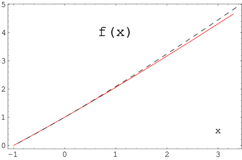
Figure 1: The scaling function $f(x)$ of the three-dimensional Ising model. The dashed line was taken from reference Guida .

V Fitted Exponents

Although one of the chief advantages of the present methodology is the fact that it is completely self-contained, in that there are no parameters to be fixed by appealing to exogenous information, as in standard parametric approaches, it is possible adapt the present method to utilize information that is available, such as precise estimates for the critical exponents and amplitude ratios. To illustrate this here, we once again consider the case $N=1$. We take the one-loop “crossover” function $(1+z^{-2})$ to give the exact form of the crossover and fit its asymptotic value to the best estimates for the critical exponents. Hence, we take

$$\gamma_{\lambda}=\frac{(4-d)}{(1+{1\over z^{2}})}\ \ \ \ \gamma_{\varphi^{2}}=\frac{(2-1/\nu)}{(1+{1\over z^{2}})}\ \ \ \ \gamma_{\varphi}=\frac{\eta}{(1+{1\over z^{2}})}$$ (75)

The crossover form for $\eta$ is of course a pure supposition given that the form $(1+z^{-2})$ is derived from a one-loop calculation. The form of (75) is such as to guarantee a crossover to the known asymptotic behavior. The same procedure could be carried out using a two-loop calculation. In this case the crossover functions for each Wilson function would be different, due to the fact that different diagrams contribute to them. Once again constants would be introduced to ensure a crossover in the limit $z\rightarrow\infty$ to the correct exponent values for $\nu$ and $\eta$. With the ansatz (75) one finds

$$\mathcal{F}(z)=\left(\frac{\nu}{\beta}\right)^{1\over 2\beta}{2\beta(\gamma-1)\over 1-2\beta}$$

$$\left[\left({\gamma(1-2\beta)\over 2\nu(\gamma-1)}z^{2}-1\right)\left(1+{\beta\over\nu}z^{2}\right)^{{1\over 2\beta}-1}+1\right]$$ (76)

$$\mathcal{G}(z)=z^{\gamma\over\beta}\left(1+{\nu\over\beta z^{2}}\right)^{(\gamma-2\beta)\over 2\beta}$$ (77)

Examining the large $z$ limit one determines the universal amplitude $A_{1}$ to be

$$A_{1}=\left(\frac{\nu}{\beta}\right)^{1\over 2\beta}{2\beta(\gamma-1)\over 1-2\beta}$$ (78)

Consequently, we determine $z_{c}^{2}=2\nu(\gamma-1)/\gamma(1-2\beta)$ and

$$A_{3}={2\beta(\gamma-1)\over(\gamma-2\beta)}\left(2\nu(\gamma-2\beta)\over 2\gamma\beta(1-2\beta)\right)^{\gamma\over 2\beta}$$ (79)

Using this mechanism, in the third column of Table 5, we show the results for the three-dimensional Ising model. The values of the critical exponents that we have used are the best values reported in the literaturePelisseto . i.e. $\gamma=1.2372$, $\beta=0.3265$ and $\nu=0.6301$.

Table 5: Numerical values of expansion coefficients for the three-dimensional Ising universality class: $HT$ results taken from referencePelisseto , one loop($RG1$) and fitted exponents ($RGA$) results. The resulting values for the coefficients $r_{2n}$ were obtained from the relation (8) and using the values of $f_{n}^{\infty}$.

	$HT$	$RG1$	$RGA$
$f_{0}^{\infty}$	0.6024(15)	0.606	0.596
$f_{1}^{\infty}$		0.696	0.793
$f_{2}^{\infty}$		0.6	0.613
$f_{3}^{\infty}$		0.223	0.151
$f_{4}^{\infty}$		-0.066	-0.084
$f_{5}^{\infty}$		-0.0454	0.00527
$r_{6}$	2.056(5)	2.5	1.938
$r_{8}$	2.3(1)	5.833	2.505
$r_{10}$	-13(4)	-17.5	-12.599
$r_{12}$		-192.5	10.902
$f_{1}^{0}$	1.0527(7)	1.034	1.05
$f_{2}^{0}$	0.0446(4)	0.029	0.043
$f_{3}^{0}$	-0.0254(7)	-0.0034	-0.0054
$f_{4}^{0}$		0.0007	0.0013
$f_{5}^{0}$		-0.00019	-0.0004
$f_{1}^{\rm c}$	0.9357(11)	0.96	0.939
$f_{2}^{\rm c}$	0.08(7)	0.048	0.076
$f_{3}^{\rm c}$		-0.0112	-0.023
$f_{4}^{\rm c}$		0.0049	0.0138
$f_{5}^{\rm c}$		-0.0028	-0.011
$R_{4}^{+}$	7.81(2)	6.892	7.981
$F_{0}^{\infty}$	0.03382(15)	0.0347	0.0263

Most of the values found with fitted exponents substantially improve the value compared with the one-loop approximation in those cases where a comparison can be made with HT expansions. This is particularly notable in $r_{6}$, $r_{8}$ and $r_{10}$. $f_{0}^{\infty}$ and $F_{0}^{\infty}$ are a little puzzling in this respect. However, it is worth noting the experimental result reported in referencePelisseto where $f^{\infty}_{0}=0.5917$, this being substantially different to the theoretical value of $f^{\infty}_{0}=0.6369$Pelisseto . The only other notable change is that of $f_{5}^{\infty}$, which is related to $r_{12}$, where there is a sign change passing from the one-loop to the adjusted values.

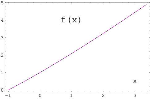
Figure 2: The scaling function $f(x)$ of the three-dimensional Ising model using fitted exponents. The dashed line was taken from reference Guida . Differences are not visible at this scale.

Table 6: Numerical values of expansion coefficients for the two-dimensional Ising universality class; high precision ($HT$) results taken from referencePelisseto and results from using fitted exponents($RGA$)

. $HT$ $RGA$ $f_{0}^{\infty}$ 0.14753 0.1043 $f_{1}^{\infty}$ 0.1696 $f_{2}^{\infty}$ 0.2365 $f_{3}^{\infty}$ 0.2931 $r_{6}$ 3.67867(7) 2.8571 $r_{8}$ 26.041(11) 15.2381 $r_{10}$ 284.5(2.4) 125.714 $r_{12}$ $4.2(7)\times 10^{3}$ 1436.73 $f_{1}^{0}$ 1.1724 $f_{2}^{0}$ 0.1473 $f_{3}^{0}$ -0.0164 $f_{1}^{c}$ 0.785 $f_{2}^{c}$ 0.295 $R_{4}^{+}$ 7.336774(10) 9.7594 $F_{0}^{\infty}$ $5.92357(6)\times 10^{-5}$ 0.10067

In the same way, we can also substitute the well-known exact values for the critical exponents in the two-dimensional case, i.e. $\gamma=7/4$, $\beta=1/8$ and $\nu=1$. Table 6 shows the subsequent results. In this case, except for the value of $f_{0}^{\infty}$, the values found for $r_{2n}$ show significant differences. This probably hints at the inadequacy of the ansatz for the crossover functions (75). We have not been able to find reported values for the coefficients $f_{n}^{0}$ and $f_{n}^{c}$, some of which are reported in Table 6. It would be interesting to be able to make the comparison.

VI Conclusions

Using environmentally friendly renormalization we derived a formal expression for the equation of state for the $O(N)$ model. This expression has the advantages that: i) it is derived from an underlying microscopic (field-theoretic) model; ii) requires as input for any calculation only the three crossover Wilson functions associated with a magnetization-dependent renormalization of the field, $\varphi$, the composite operator, $\varphi^{2}$, and the coupling constant, $\lambda$. In particular no experimental input is required on order to fix parameters; iii) it is parameterized by two non-linear scaling fields - the transverse mass, and an anisotropy parameter closely related to the stiffness constant; iv) it manifestly expresses all relevant, desired analyticity properties, both in the critical region and on the coexistence curve; v) universal coefficients associated with the expansion of the equation of state in any of the asymptotic regimes may be simply calculated thereby obtaining coefficients that are presently unknown.

After deriving one-loop expressions for general $N$, the formulation was then used to calculate a parameterized, analytic expression for the equation of state for $N=1$ for $2<d<4$. For $d=3$ it was shown how the parameterization could be dispensed with and a closed-form, non-parameterized expression for the equation of state derived. Various universal coefficients associated with the asymptotic regimes $x=0$, $x=\infty$ and $x=-1$ were derived for arbitrary $d$. For $d=3$ these were compared with previous results.

By taking the functional form for the Wilson functions at one-loop and introducing constants to fit to the best-known asymptotic values of the critical exponents, comparison was made for $d=3$ and $d=2$ between our calculated expansion coefficients and those, where known, as derived using HT expansions, Monte Carlo, etc., in the different asymptotic regimes. In most cases the fitted values were substantially better than the one-loop values, agreement being better for $d=3$ than $d=2$.

When continued to complex values of the external magnetic field the universal equation of state should also capture the Lee-Yang edge. There are additional points of non-analyticity in our expressions at $z^{2}_{LY}=-2/(d-2)$ or $z^{2}_{LY}=-\nu/\beta$. These imaginary values of $z$ are naturally associated with the Lee-Yang edge singularities. However, our equation of state is not yet optimized to include the associated crossover and we do not expect to obtain good estimates for the associated universal exponents or amplitudes. Our formulation can be adjusted to include this additional singularity, but as of yet we have not studied the effect of including this crossover. We hope to return to this in the future.

References

- (1) J. Zinn-Justin, Physics Reports 344, 159-179 (2001).
- (2) I. D. Lawrie, J. Phys. A: Math. Gen. 14, 24898, (1981).
- (3) B. Nienhuis and M. Nauenberg, Phys. Rev. Lett. 35, 477 (1975).
- (4) N. Berker and M.E. Fisher, Phys. Rev. B26, 2507 (1982).
- (5) L. Schäfer and H. Horner, Z. Phys. B 29, 251 (1978).
- (6) J. Berges, N. Tetradis and C. Wetterich, Phys. Rev. Lett. 77, 873, (1996).
- (7) B. Widom, J. Chem. Phys. 43, 3898 (1965).
- (8) R. Guida and J. Zinn-Justin, Nucl. Phys. B489, 626, (1997).
- (9) D. O’Connor and C. R. Stephens, Phys. Rept. 363, 425 (2002).
- (10) J.K. Kim and D.P. Landau, Nucl. Phys.B (Proc.Suppl.) 53, 706, (1997).
- (11) A. Pelissetto and E Vicari, Phys. Rept. 368, 549 (2002). See also M. Campostrini, A. Pelissetto, P. Rossi and E. Vicari. Phys. Rev. B 62, 5843 (2000)
- (12) J. Engels, S. Holtmann, T. Mendes and T. Schulze, Phys. Lett. B492, 219 (2000).
- (13) P. Schofield, Phys. Rev. Lett. 22, 606 (1969).
- (14) E. Brézin, D.J. Wallace and K. G. Wilson, Phys. Rev. B7, 232 (1973).
- (15) D.J. Wallace and R.K.P. Zia, Phys. Rev. B12 ,5340 (1975).
- (16) R. B. Griffiths, Phys. Rev. 158, 176 (1967).