Ambiguities in the scattering tomography for central potentials

Abstract

Invisibility devices exploit ambiguities in the inverse scattering problem of light in media. Scattering also serves as an important general tool to infer information about the structure of matter. We elucidate the nature of scattering ambiguities that arise in central potentials. We show that scattering is a tomographic projection: the integrated scattering angle is a projection of a scattering function onto the impact parameter. This function depends on the potential, but may be multi-valued, allowing for ambiguities where several potentials share the same scattering data. In addition, multivalued scattering angles also lead to ambiguities. We apply our theory to show that it is in principle possible to construct an invisibility device without infinite phase velocity of light.

An invisibility device Gbur ; Pendry ; LeoConform ; LeoNotes ; Kerker ; Others should guide light around an object as if nothing were there. It is conceivable that such devices can be made using modern metamaterials Pendry ; LeoConform ; LeoNotes ; Others . Passive optical devices use spatially varying refractive-index profiles for imaging. Within the validity range of geometrical optics, index profiles of isotropic dielectric media are mathematically equivalent to potentials for light rays BornWolf ; LeoNotes . Therefore, such an invisibility device corresponds to a potential that has the same scattering characteristic as empty space. While the inverse scattering problem for waves has unique solutions Nachman , the scattering of rays may be ambiguous. Here we show how such ambiguities arise in the case of radially symmetric potentials. Our theory indicates that it is in principle possible to construct an invisibility device where the phase velocity of light does not approach infinity, in contrast to all previous proposals for macroscopic cloaking Pendry ; LeoConform ; LeoNotes . This could inspire ideas for developing invisibility devices without anomalous dispersion Pendry that could operate in a relatively wide frequency window. In addition to applications in a potentially new area for metamaterials, our theory has wider implications for the field of scattering tomography.

The inversion of the classical scattering in central potentials is a classic textbook problem that has made it into the exercises in Landau’s and Lifshitz’ Mechanics LLproblem . Since Rutherford’s experiments, scattering has served as an important tool to investigate the structure of matter, with modern applications ranging from biomedical research to astrophysics. Techniques to infer the structure of matter from scattering are often called scattering tomography, although, strictly speaking, they are not directly related to traditional tomography Tomo where the shape of a hidden object is reconstructed from projections. Here we show that the case of scattering in central potentials literally is a tomographic projection in disguise, but with an interesting twist: the object to be reconstructed corresponds to the potential, but may be represented by a multi-valued function, allowing for ambiguities.

Figure 1: Scattering in a central potential. A trajectory incident with impact parameter $b$ is deflected by the angle $\chi$ in the rotationally symmetric potential $U(r)$ centered at the origin, with $r=\sqrt{x^{2}+y^{2}}$ in the Cartesian coordinates $x$ and $y$. The turning point of the trajectory is denoted by $r_{0}$. The figure shows Rutherford scattering LL1 in a repulsive $1/r$ potential.

Figure 1 illustrates the situation typical for scattering in central potentials. An incident ray characterized by the impact parameter $b$ and the energy $E$ is deflected by the angle $\chi$. We use polar coordinates with radius $r$ and angle $\varphi$ in the plane orthogonal to the angular-momentum vector. The scattering angle is determined as LL1

$$\chi=\pi-2\int_{r_{0}}^{\infty}\frac{(b/r)\,dr}{\sqrt{\rho^{2}-b^{2}}}\,.$$ (1)

Here $r_{0}$ denotes the turning point of the trajectory given by $b$ and $E$, and $\rho$ represents the potential as

$$\rho=r\sqrt{1-\frac{U(r)}{E}}\,,\quad\frac{U}{E}=1-\frac{\rho^{2}}{r^{2}}\,.$$ (2)

The turning point is given by the largest value of $r$ at which the denominator in the integrand (1) of the scattering angle vanishes, i.e. at which $\rho=b$. Reversing this relation leads to a physical interpretation for $\rho$: $\rho(r)$ describes the impact parameter for which the radius $r$ is a turning point. Therefore we may call $\rho$ turning parameter. Figure 2 illustrates the representation of the potential using the turning parameter.

Figure 2: Representation of the potential by the turning parameter $\rho$ defined in Eq. (2). The solid line in A shows a potential with a fold in the turning parameter where $r(\rho)$ is multi-valued. Subfigure B shows the corresponding potential $U(r)$. The dotted lines describe $\rho(r)$ and $U(r)$ for a potential with the same scattering characteristics. Here $r(\rho)$ was obtained from Eq. (10) using the definition (5) of the scattering function $W$.

The largest zero of $\rho(r)$ corresponds to the potential barrier where $U=E$. The potential is repulsive for $\rho<r$, zero for $\rho=r$ and attractive for $\rho>r$. Note that the inverse function $r(\rho)$ may be multi-valued, as shown in Fig. 2A. The additional values of $r(\rho)$ describe the turning points of additional bound trajectories for the same energy $E$ and the angular momentum that corresponds to the impact parameter $b$. Scattering does not probe such bound states, although the trajectories of scattered rays may enter the same region for different impact parameters $b$. As we show, the possibility of such elusive bound trajectories indicates ambiguities in scattering.

In the following, we express the description of scattering in central potentials as a tomographic projection for the integrated scattering angle

$$\phi=\int_{\infty}^{b}\chi\,db\,.$$ (3)

First, we represent Eq. (1) as

$$\chi = 2b\left(\int_{b}^{\infty}\frac{d\rho}{\rho\sqrt{\rho^{2}-b^{2}}}-\int_{r_{0}}^{\infty}\frac{dr}{r\sqrt{\rho^{2}-b^{2}}}\right)$$ (4)

$$= 2b\int_{b}^{\infty}\frac{W^{\prime}}{a}\,d\rho$$

in terms of

$$W=\ln(\rho/r)\,,\quad a=\sqrt{\rho^{2}-b^{2}}\,.$$ (5)

A prime indicates differentiation with respect to the turning parameter. We call $W$ scattering function. When $r(\rho)$ is multi-valued the integration contour is understood to follow accordingly. Since

$$\frac{d}{db}\int_{b}^{\infty}W^{\prime}a\,d\rho+\int_{b}^{\infty}\frac{W^{\prime}b}{a}\,d\rho=\left.-W^{\prime}a\right|_{\rho=b}=0\,,$$ (6)

we obtain for the integrated scattering angle

$$\phi=-2\int_{b}^{\infty}W^{\prime}a\,d\rho=2\int_{b}^{\infty}Wa^{\prime}\,d\rho=\int_{-\infty}^{+\infty}Wda\,.$$ (7)

This result has a simple geometrical meaning illustrated in Fig. 3:

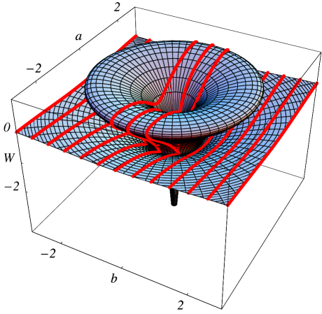
Figure 3: Scattering tomography. The integrated scattering angle $\phi$ is a projection of the scattering function $W$ onto the impact parameter $b$ along the red lines of the fictitious parameter $a$. The radius $\rho$ in this auxiliary $(a,b)$ plane is the turning parameter (2). The scattering function, defined in Eq. (5) and obtained from Fig. (2), may be multi-valued, as shown here. The folds of $W$ visualize the ambiguities of scattering.

imagine that $a$ and $b$ constitute a plane of impact parameters where one, $b$, is experimentally accessible and the other, $a$, is not. The scattering function $W$ depends only on the radius $\rho=\sqrt{a^{2}+b^{2}}$, both directly by definition (5) and in $r(\rho)$. Equation (7) shows that the integrated scattering angle is a projection of the rotationally symmetric object $W(\rho)$ onto the experimentally accessible impact parameter $b$ in exactly the same way as objects are projected in classical tomography Tomo or Wigner functions in quantum tomography Leo ; LeoJex . If $r(\rho)$ is single-valued, one can invert the projection by the inverse Abel transformation Leo ; LeoJex

$$W=-\frac{1}{\pi}\int_{\rho}^{\infty}\frac{\chi\,db}{\sqrt{b^{2}-\rho^{2}}}\,,$$ (8)

a special case of the inverse Radon transformation Leo . If $r(\rho)$ is multi-valued one can hide features of the potential in the folds of $W$, as Fig. 3 illustrates.

Consider the scattering ambiguities where the scattering function $W$ is multi-valued. The simplest case corresponds to a single fold in $W$ between two turning parameters $\rho_{1}$ and $\rho_{2}$, as shown in Figs. 3 and 4.

Figure 4: Multi-valued scattering function $W$ obtained from Fig. (2) according to the definition (5). The $W(\rho)$ function is folded between the turning parameters $\rho_{1}$ and $\rho_{2}$ where $W_{+}$ denotes the top and $W_{-}$ the bottom curve of the fold.

We use the inverse Abel transformation (8) to construct a potential, described by $W_{0}(\rho)$, that exhibits the same scattering characteristics as $W$. Figure 3 indicates that $W$ and $W_{0}$ agree for $\rho>\rho_{1}$, because all projections lie under the fold. For $\rho<\rho_{1}$ the scattering angle $\chi$ is, according to Eq. (1),

$$\chi=2b\int_{b}^{\infty}\frac{W^{\prime}d\sigma}{\sqrt{\sigma^{2}-b^{2}}}+2b\int_{\rho_{1}}^{\rho_{2}}\frac{W^{\prime}_{+}-W^{\prime}_{-}}{\sqrt{\sigma^{2}-b^{2}}}\,d\sigma\,.$$ (9)

where the integration variable $\sigma$ refers to the turning parameter, $W$ follows the solid curve in Fig. 4, with a jump at $\rho_{1}$, whereas $W_{+}$ denote the top and $W_{-}$ the bottom curve of the fold. Since the inverse Abel transformation (8) uniquely inverts the first term in $\chi$, we obtain for the difference between $W$ and $W_{0}$

$$W-W_{0} = \frac{2}{\pi}\int_{\rho}^{\rho_{1}}\int_{\rho_{1}}^{\rho_{2}}\frac{b\,(W^{\prime}_{+}-W^{\prime}_{-})\,d\sigma\,db}{\sqrt{(b^{2}-\rho^{2})(\sigma^{2}-b^{2})}}$$ (10)

$$= \frac{2}{\pi}\int_{\rho_{1}}^{\rho_{2}}(W^{\prime}_{+}-W^{\prime}_{-})\,\arctan\left(\frac{\sqrt{\rho_{1}^{2}-\rho^{2}}}{\sqrt{\sigma^{2}-\rho_{1}^{2}}}\right)d\sigma$$

$$= \frac{2}{\pi}\int_{\rho_{1}}^{\rho_{2}}(W_{+}-W_{-})\,\frac{\sqrt{\rho_{1}^{2}-\rho^{2}}}{\sqrt{\sigma^{2}-\rho_{1}^{2}}}\,\frac{\sigma\,d\sigma}{\sigma^{2}-\rho^{2}}$$

by partial integration, utilizing that the boundary term vanishes, because $W_{-}(\rho_{2})=W_{+}(\rho_{2})$. Since $W_{+}>W_{-}$ the ambiguous $W$ must exceed $W_{0}$ in the single-valued region inside $\rho_{1}$, which implies that the radius $r=\rho\,\exp(-W_{0})$ is greater than $\rho\,\exp(-W)$. The fold of multi-valuedness thus magnifies the scattering structure of the potential. In particular, for ambiguous scattering potentials, the zero of $\rho(r)$ is closer to the origin than for the equivalent non-ambiguous one. Since this zero corresponds to the potential barrier beyond which one can hide, nothing is gained, quite the opposite. This feature continues in the general case of several folds in $W$, because one could replace $W$ by equivalent single-valued $W_{0}$ with the same scattering characteristics, starting from the outmost fold and proceeding to the inside.

An alternative way of hiding the presence of a potential would be to let the trajectories leave at scattering angles that are multiples of $2\pi$, i.e to turn them around in precisely adjusted loops. Suppose that for impact parameters $b$ smaller than a critical $b_{0}$ the trajectories are uniformely turned by $\chi=-2\pi\nu$ and are not affected for $b$ larger than $b_{0}$. Here $\nu$ may be a real number, not only an integer, for the sake of generality. Assuming that $r(\rho)$ is single-valued, we obtain from the inverse Abel transformation (8)

$$r=\left\{\begin{array}[]{lcl}\rho\left({b_{0}}/{\rho}+\sqrt{{b_{0}^{2}}/{\rho^{2}}-1}\right)^{-2\nu}&:&\rho<b_{0}\\ \rho&:&\rho\geq b_{0}\end{array}\right.\,.$$ (11)

Figure 5 illustrates the curves of $\rho(r)$. Clearly, $r(\rho)$ is single-valued by definition. For $\nu<0$ the potential would be repulsive, because the trajectories are deflected, but in this case the function $\rho(r)$ itself is multivalued. Consequently, no central potential exists that uniformly deflects trajectories. For $\nu>0$ the potential is attractive, as one would expect to be necessary for bending trajectories around the center of force. The case $\nu=1/2$ corresponds to a Kepler potential LL1 or the Eaton lens KerkerScattering developed in radar technology. In the limit $\rho\rightarrow 0$ we get from Eq. (11) the asymptotics $\rho/r\sim(2/r)^{2\nu/(2\nu+1)}$, and hence, according to Eq. (2) the potential $U$ diverges with the power $-4\nu/(2\nu+1)$ for small $r$. One cannot hide anything here. In the limit $\nu\rightarrow\infty$ of infinitely many cycles $U$ approaches near the origin the $1/r^{2}$ potential of fatal attraction LL1 . Figure 5B illustrates the case where the trajectories are turned around by $2\pi$.

Figure 5: Uniform bending. Subfigure A shows the turning parameters obtained from Eq. (11) for the winding numbers $\nu\in\{2,1,0.5,-0.1,-0.2,-0.3\}$ and $b_{0}=1$. For negative $\nu$, $\rho(r)$ is multi-valued and hence unphysical. Subfigure B illustrates the uniform loops of trajectories for $\nu=1$.

Although one cannot directly apply the ambiguous scattering of isotropic and centrally symmetric media to construct an invisibility device, one can use their singularities to improve anisotropic devices. Such a device is designed to facilitate a coordinate transformation with a hole Pendry . Anything inside the hole is hidden by construction Pendry . Consider a two-dimensional case in polar coordinates. Suppose that the radius $r$ is mapped onto $r^{\prime}$ such that $r^{\prime}$ reaches the radius of the hole at $r=0$ as

$$\frac{\partial r^{\prime}}{\partial r}\sim\alpha r^{-s}\quad\mbox{for}\quad r\sim 0\,,$$ (12)

where $\alpha$ and $s$ are non-negative constants. Beyond the outer radius $b_{0}$ of the cloak the coordinates $r^{\prime}$ shall coincide with $r$. Assume in unprimed space the isotropic and radially symmetric refractive-index profile $n(r)$ with perfect impedance matching. Reference Pendry gives a recipe to calculate the dielectric $\varepsilon$ and magnetic $\mu$ that facilitates the coordinate transformation (12). We find

$$\varepsilon_{r}^{\prime}=\mu_{r}^{\prime}\sim\frac{\alpha r^{1-s}}{r^{\prime}}\,n(r)\,,\quad\varepsilon_{\varphi}^{\prime}=\mu_{\varphi}^{\prime}\sim\frac{r^{s-1}}{\alpha r^{\prime}}\,n(r)\,.$$ (13)

Suppose that we use a profile where $n^{2}/2$ corresponds LeoNotes to the $E-U$ of uniform bending (11) with the definition (2) and $\nu=1$. If we choose $s=1/3$ the singularity of $U$ compensates for the zero in the refractive index in real space that would otherwise imply Pendry that the speed of light tends to infinity at the inner surface of the cloak. The phase velocity in radial direction is finite. On the other hand, the speed of light in angular direction tends to zero with the power $4/3$. Our simple example indicates that invisibility devices with finite phase velocity are possible in principle. In our case, wrapping light around the invisibility device stratifies the optical wavefronts. However, there is a price to pay: light propagation with finite phase velocity around an object inevitably causes time delays that result in wavefront dislocations at the boundary LeoNotes . The invisibility is perfect for rays, but not for waves.

Conclusions.— Scattering in central potentials corresponds to a tomographic projection that visualizes scattering ambiguities. Such ambiguities are limited, though: central potentials are not suitable to achieve the same scattering characteristics as empty space. Therefore, highly asymmetric refractive-index profiles LeoConform ; LeoNotes or highly anisotropic media Pendry are required to design invisibility devices, which, interestingly, can operate with a finite speed of light. Otherwise, trying to hide things uniformly from all sides just magnifies them.

The paper was supported by the Alexander von Humboldt Foundation, the Leverhulme Trust and King Saud University.

References

- (1) G. Gbur, Prog. Opt. 45, 273 (2003).
- (2) J. B. Pendry, D. Schurig and D. R. Smith, Science Express, May 25 (2006).
- (3) U. Leonhardt, arXiv:physics/0602092, Science Express, May 25 (2006).
- (4) U. Leonhardt, arXiv:physics/0605227.
- (5) M. Kerker, J. Opt. Soc. Am. 65, 376 (1975).
- (6) A. Alu and N. Engheta, Phys. Rev. E 72, 016623 (2005); G. W. Milton and N.-A. P. Nicorovici, Proc. Roy. Soc. London A 462, 1364 (2006).
- (7) M. Born and E. Wolf, Principles of Optics (Cambridge University Press, Cambridge, 1999).
- (8) A. I. Nachman, Ann. Math. 128, 531 (1988).
- (9) Problem 7 in $18 of Ref. LL1 .
- (10) G. T. Herman, Image Reconstruction from Projections: The Fundamentals of Computerized Tomography (Academic, New Yortk, 1980); F. Natterer, The Mathematics of Computerized Tomography (Wiley, Chichester, 1986).
- (11) L. D. Landau and E. M. Lifshitz, Mechanics (Pergamon, Oxford, 1976).
- (12) U. Leonhardt, Measuring the Quantum State of Light (Cambridge University Press, Cambridge, 1997).
- (13) U. Leonhardt and I. Jex, Phys. Rev. A 49, R1555 (1994).
- (14) M. Kerker, The Scattering of Light (Academic Press, New York, 1969).