Bosonic representation of spin operators in the field-induced critical phase of spin-1 Haldane chains

Abstract

A bosonized-field-theory representation of spin operators in the uniform-field-induced Tomonaga-Luttinger-liquid (TLL) phase in spin-1 Haldane chains is formulated by means of the non-Abelian (Tsvelik’s Majorana fermion theory) and the Abelian bosonizations and Furusaki-Zhang technique [Phys. Rev. B 60, 1175 (1999)]. It contains massive magnon fields as well as massless boson fields. From it, asymptotic forms of spin correlation functions in the TLL phase are completely determined. Applying the formula, we further discuss effects of perturbations (bond alternation, single-ion anisotropy terms, staggered fields, etc) for the TLL state, and the string order parameter. Throughout the paper, we often consider in some detail how the symmetry operations of the Haldane chains are translated in the low-energy effective theory.

1 Introduction

For (quasi) one-dimensional (1D) magnets, sophisticated theoretical tools have been developed in the last decades; for example, bosonizations [1, 2, 3], conformal field theory (CFT) [4], Bethe ansatz [5, 6], and several numerical methods (exact diagonalization, density-matrix renormalization group (DMRG), quantum Monte Carlo method (QMC), etc). Thanks to them, we have obtained a deep understanding of 1D spin systems. Of course, they have succeeded in explaining a number of experimental results of quasi 1D magnets. In this paper, we try to further develop a low-energy field theory description for spin-1 antiferromagnetic (AF) chains in a uniform magnetic field, which are a fundamental model in 1D spin systems.

Before discussing spin-1 AF chains, for comparison, let us briefly review the well-established low-energy effective theory (so-called Abelian bosonization) for the spin-1/2 XXZ chain [7, 8], which is one of the well-investigated and realistic models in spin systems. The Hamiltonian is defined by

$$\hat{\cal H}_{\rm xxz} = J\sum_{j}\left[\frac{1}{2}(S_{j}^{+}S_{j+1}^{-}+{\rm h.c.})+\Delta_{z}S_{j}^{z}S_{j+1}^{z}\right]-H\sum_{j}S_{j}^{z},$$ (1)

where $\vec{S}_{j}$ is spin-1/2 operator on site $j$, $J>0$ is the exchange interaction, $\Delta_{z}$ is the anisotropy parameter ($\Delta_{z}=1$ case is the SU(2) Heisenberg chain), and $H\geq 0$ is a uniform field. In a wide parameter regime including the zero-field line ($1<\Delta_{z}\leq 1$ and $H=0$) [3, 8], the low-energy physics is governed by a one-component Tomonaga-Luttinger liquid (TLL) phase, where the spin correlation functions are of an algebraical decay type. For this critical phase, a beautiful field theory description has been established as follows. The low-energy effective Hamiltonian is a massless Gaussian model,

$$\hat{\cal H}_{\rm xxz}^{\rm eff} = \int dx\frac{\bar{v}}{2}\left[{\bar{K}}(\partial_{x}{\bar{\theta}})^{2}+\frac{1}{\bar{K}}(\partial_{x}{\bar{\phi}})^{2}\right],$$ (2)

where $x=j\times a_{0}$ ($a_{0}$ is the lattice constant), $\bar{\phi}(x)$ is the scalar bosonic field, $\bar{\theta}(x)$ is the dual of $\bar{\phi}$, $\bar{v}$ is equal to the massless spinon velocity of the chain (1), and $\bar{K}$ is the TLL parameter ($\bar{K}=1$ and $\bar{K}=1/2$ respectively correspond to the XY (free fermion) point $\Delta_{z}=0$ and the SU(2) Heisenberg one $\Delta_{z}=1$) [9]. In this effective theory framework, the spin operator $\vec{S}_{j}$ is approximated [3, 7, 8, 10] as

$$S_{j}^{z}/a_{0} \approx \frac{\bar{M}}{a_{0}}+\frac{1}{\sqrt{\pi}}\partial_{x}{\bar{\phi}}+(-1)^{j}A_{1}^{z}\sin\left(\sqrt{4\pi}{\bar{\phi}}+2\pi\bar{M}\frac{x}{a_{0}}\right)+\cdots,$$

$$S_{j}^{+}/a_{0} \approx e^{i\sqrt{\pi}\bar{\theta}}\left[(-1)^{j}A_{0}+A_{1}\sin\left(\sqrt{4\pi}{\bar{\phi}}+2\pi\bar{M}\frac{x}{a_{0}}\right)+\cdots\right],$$ (3)

where $\bar{M}$ is the magnetization per site $\langle S_{j}^{z}\rangle$, and $A_{n}$ and $A_{n}^{z}$ are nonuniversal real constants. The magnetization $\bar{M}$, the velocity $\bar{v}$, and the TLL parameter $\bar{K}$ can be determined as a function of the parameters $(J,\Delta_{z},H)$, via the Bethe ansatz integral equations for the XXZ chain. If these three parameters are given, one can correctly know the asymptotic behavior of any spin correlation functions through the formula (1). Since the accurate values of $A_{n}$ and $A_{n}^{z}$ have recently been estimated [11, 10], it is also possible to obtain the amplitudes of the spin correlation functions. This effective theory, especially the bosonized spin formula (1), is very useful in analyzing not only the XXZ chain itself, but also several perturbation effects (bond alternations, next-nearest-neighboring interactions, anisotropy terms, etc) for the XXZ chain and coupled spin-1/2 chain systems.

Now, we turn to spin-1 AF chains and their effective theories. In this paper, we mainly consider the following simple spin-1 AF Heisenberg chain,

$$\hat{\cal H}_{S=1} = J\sum_{j}\vec{S}_{j}\cdot\vec{S}_{j+1}-H\sum_{j}S_{j}^{z},$$ (4)

where $\vec{S}_{j}$ is “spin-1” operator on site $j$. In contrast to the spin-1/2 case, the spin-1 AF chain (4) without a uniform field ($H=0$) possesses a finite excitation gap (call Haldane gap) on its disordered ground state, which is described by the famous valence-bond-solid picture [12]. The low-lying excitation consists of a massive spin-1 magnon triplet around wave number $p=\pi/a_{0}$. The spin correlation functions exhibit an exponential decay. This drastic difference between the spin-1/2 and spin-1 cases was first predicted by Haldane in 1983 [13]: he developed the nonlinear sigma model (NLSM) approach [14, 15, 7] for spin systems in order to explain the above low-energy physics of the spin-1 chain. After Haldane’s conjecture, based on the non-Abelian bosonization approach to 1D spin systems [16, 17, 18], Tsvelik proposed a Majorana (real) fermion theory [19, 1, 2, 20], which also has an ability to demonstrate the low-energy properties of the spin-1 AF chains. Both theories are now a standard field theory method of studying 1D spin-1 AF systems [21], like the Abelian bosonization for spin-1/2 chains.

When a uniform field $H$ is applied in the spin-1 SU(2) AF chain (4), the low-lying magnon bands are split due to the Zeeman coupling. Provided that the bottom of one band crosses the energy level of the disordered ground state, a magnon condensed state and a finite magnetization occur [22, 23, 24, 25]. It is well known that this quantum phase transition is of a commensurate-incommensurate (C-IC) type [26, 3], and the resultant phase can be regarded as a TLL. Therefore, it is expected that, just like the formula (1), one can obtain a bosonized-spin expression in this TLL phase. However, as far as we know, any clear bosonization formulas of spin-1 operators in this magnon-condensed phase have not been established yet. Namely, such a formula has not been argued enough so far [27].

The main purpose of this paper is to derive a satisfactory bosonization formula for spin-1 operators in the above TLL phase. To this end, we start with Tsvelik’s Majorana fermion theory. This theory makes it possible to treat the Zeeman term in a nonperturbative way. Moreover, it can carefully deal with the uniform component of spins (the part around wave number $p\sim 0$) as well as the staggered ones, in contrast to the NLSM approach. (We explain these properties of the fermion theory in later sections). To make the new bosonization formula, the bosonized-spin expression for the uniform-field-induced TLL phase in a two-leg spin-1/2 AF ladder [28] and its derivation, which was performed by Furusaki and Zhang [29], is very instructive and helpful. We will rely on these results. We will often discuss the symmetry correspondences between the original spin-1 AF chain (4) and the effective field theory. Like the formula (1), our resulting formula would be powerful in studying various (quasi) 1D spin-1 AF systems with magnons condensed. Recently, magnon-condensed states in quasi 1D gapped magnets, including spin-1 compounds such as NDMAP [30, 31, 32, 33, 34, 35], NDMAZ [36], TMNIN [37] and NTENP [38, 39], have been intensively investigated by some experiment groups. Our new formula hence is expected to be effective for understanding results of such experiments.

The organization of the rest of the paper is as follows. In Sec. 2, we review Tsvelik’s Majorana fermion theory for the spin-1 AF chain without external fields. Section 3 is devoted to discussing the effective field theory for the uniform-field-induced TLL in spin-1 AF chains, which is based on the Majorana fermion theory. These two sections are needed as the preparation to construct a field-theory formula for spin operators in the TLL phase, although several parts of them have been already discussed in literature [1, 2, 19, 20, 40]. In Sec. 4, which is the main content of this paper, employing the contents of Secs. 2 and 3, we derive the formula of spin operators. Moreover, using it, we estimate the asymptotic forms of spin correlation functions in the TLL phase. Section 5 provides easy applications of our field-theory formula of spin operators. We consider the nonlocal string order parameter [41, 40], effects of some perturbation terms (bond alternation, a few anisotropy terms, etc) for the TLL state, and the magnon-decay process caused by anisotropic perturbations. We summarize the results of this paper in Sec. 6. Appendices may prove useful when reading the main text.

2 Spin-1 AF chain without external fields

In this section, we review the non-Abelian bosonization (Tsvelik’s Majorana fermion theory) method for the spin-1 Heisenberg AF chain with $H=0$, especially focusing on the symmetries of the chain.

2.1 WZNW model and Majorana fermion theory

First, we define the spin-1 bilinear-biquadratic chain,

$$\hat{\cal H}_{\beta} = J\sum_{j}\left[\vec{S}_{j}\cdot\vec{S}_{j+1}+\beta(\vec{S}_{j}\cdot\vec{S}_{j+1})^{2}\right].$$ (5)

Several studies [42] reveal that the system belongs to the “Haldane phase” in the regime $|\beta|<1$, and the points $\beta=\pm 1$ correspond to a quantum criticality. In the Haldane phase, the ground state is disordered (namely, all symmetries are conserved) and the lowest excitations have a finite Haldane gap on it. It is shown [16, 43, 44] that the low-energy physics of the critical point $\beta=-1$ is captured by an SU(2) level-2 Wess-Zumino-Novikov-Witten (WZNW) model [1, 2], a model of CFT with central charge $c=3/2$, plus irrelevant perturbations preserving the spin SU(2) symmetry. This WZNW model possesses a Majorana (real) fermion description, i.e., the WZNW model with $c=3/2$ is equivalent to three copies of massless real fermions, each of which is regarded as a critical Ising system (a minimal model of CFT) with $c=1/2$ [17, 28, 1, 2]. Using the fermion (or Ising) picture, one can represent the Hamiltonian of the WZNW model as follows:

$$\hat{\cal H}_{\rm wznw} = \int dx\,\frac{i}{2}v_{0}\sum_{q=1,2,3}\Big{[}\xi_{L}^{q}\partial_{x}\xi_{L}^{q}-\xi_{R}^{q}\partial_{x}\xi_{R}^{q}\Big{]},$$ (6)

where $\xi_{L(R)}^{q}(x)={\xi_{L(R)}^{q}}^{\dagger}(x)$ is the left (right) moving field of the $q$th real fermion with scaling dimension $\Delta_{s}=1/2$, and $v_{0}$ is the “light” velocity of the fermions. We here normalize the fermions $\xi_{L(R)}^{q}$ through the anticommutation relation $\{\xi_{\nu}^{q}(x),\xi_{\nu^{\prime}}^{q^{\prime}}(y)\}=\delta_{\nu,\nu^{\prime}}\delta_{q,q^{\prime}}\delta(x-y)$, where the delta function stands for $\delta_{x,y}/\alpha$ [$\alpha$ is a constant of ${\cal O}(a_{0})$]. At the WZNW point $\beta=-1$, the spin operator is approximated as the following sum of the uniform and the staggered components [16, 19, 1, 2],

$$S_{j}^{q}/a_{0}\approx J^{q}(x)+(-1)^{j}C_{0}N^{q}(x),\,\,\,\,(q=1,2,3\,\,{\rm or}\,\,x,y,z),$$ (7)

where

$$J^{q}(x)=J_{L}^{q}(x)+J_{R}^{q}(x),\hskip 14.22636ptJ_{L(R)}^{q}=-i\xi_{L(R)}^{q+1}\xi_{L(R)}^{q+2},\,\,\,(q+3=q),$$

$$\left\{\begin{array}[]{ccc}N^{1}=\mu^{1}\sigma^{2}\mu^{3}\\ N^{2}=\sigma^{1}\mu^{2}\mu^{3}\\ N^{3}=\mu^{1}\mu^{2}\sigma^{3}\end{array}\right.,$$ (11)

and $C_{0}$ is a nonuniversal constant. The quantity $J_{L(R)}^{q}$ is equivalent to the left (right) component of the SU(2) current in the WZNW model with $\Delta_{s}=1$, and $\sigma^{q}$ ($\mu^{q}$) is the $q$th-Ising order (disorder) field with $\Delta_{s}=2/16$.

According to Tsvelik [19, 18, 1, 2], transferring from the WZNW point $\beta=-1$ to the Heisenberg one $\beta=0$ corresponds to adding two SU(2)-symmetric (see the next subsection) perturbation terms, a fermion mass term and a marginally irrelevant current-current interaction, to the WZNW model (6). Namely, he proposed that the low-energy and long-distance properties of the spin-1 Heisenberg chain (4) are govern by the effective Hamiltonian,

$$\hat{\cal H}_{S=1}^{\rm eff} = \int dx\sum_{q}\left[\frac{i}{2}v_{0}\left(\xi_{L}^{q}\partial_{x}\xi_{L}^{q}-\xi_{R}^{q}\partial_{x}\xi_{R}^{q}\right)+mi\xi_{L}^{q}\xi_{R}^{q}-\lambda J_{L}^{q}J_{R}^{q}\right],$$ (12)

where we may set $m>0$ and $\lambda>0$, which guarantees the irrelevancy of the $\lambda$ term. From the viewpoint of the spin-1 AF chain, fermions $\xi_{L,R}^{q}$ stand for the low-lying magnon triplet around wave number $p=\pi/a_{0}$, the mass parameter $m$ corresponds to the Haldane gap, and the $\lambda$ term represents the inter-magnon interaction. Renormalizing the $\lambda$ interaction effect into the kinetic and the mass terms, or simply neglecting the $\lambda$ term, one can determine the values of $v_{0}$ and $m$ from the numerically-estimated magnon dispersion of the spin-1 Heisenberg chain; such a procedure provides $v_{0}\approx 2.49Ja_{0}$ and $m\approx 0.41J$ [45, 46]. One should interpret that the inequality $m>0$ corresponds to the disordered phase in the Ising-model picture, in which $\langle\mu^{q}\rangle\neq 0$ and $\langle\sigma^{q}\rangle=0$. For the disordered phase, Ising-field correlation functions [47, 28, 19] are shown to be

$$\langle\sigma^{q}(x)\sigma^{q}(0)\rangle \approx \frac{B_{1}}{\sqrt{2\pi|x|/\xi_{c}}}\left(1+{\cal O}(|x/\xi_{c}|^{-1})\right)e^{-|x|/\xi_{c}}+{\cal O}(e^{-3|x|/\xi_{c}}),$$

$$\langle\mu^{q}(x)\mu^{q}(0)\rangle \approx B_{1}\left[1-\left(\frac{1}{16\pi|x|/\xi_{c}}+{\cal O}(|x/\xi_{c}|^{-2})\right)e^{-2|x|/\xi_{c}}\right]$$ (13)

$$+{\cal O}(e^{-4|x|/\xi_{c}}),$$

at a long distance, $x\gg\xi_{c}=v_{0}/m$ [48]. Here, $B_{1}$ is a nonuniversal constant, and $\xi_{c}\approx 6a_{0}$ is the correlation length. If we assume that the field-theory formula (7) is valid even at the Heisenberg point $\beta=0$, that formula and the result (2.1) lead to the following asymptotic behavior of the spin correlation functions of the spin-1 Heisenberg chain:

$$\langle S_{j}^{q}S_{0}^{q}\rangle \approx (-1)^{j}\frac{B_{2}}{\sqrt{|x|/\xi_{c}}}e^{-|x|/\xi_{c}}+\frac{B_{3}}{|x|/\xi_{c}}e^{-2|x|/\xi_{c}}+\cdots,$$ (14)

where we used Eqs. (116dpdrdseaebecexeyezfjflgd) and (B) to derive the second term, and $B_{2,3}$ are nonuniversal constants. The exponential parts in Eq. (14) are consistent with those predicted by the NLSM approach [49], but the prefactor ($\propto 1/x$) of the second uniform term differs from that of the NLSM, which predicts a prefactor proportional to $1/x^{2}$. From the calculation of DMRG [49], we may conclude $B_{2}\approx 0.25$ and $B_{3}\ll B_{2}$.

2.2 Symmetries of the spin-1 AF Heisenberg chain

The effective Hamiltonian (12) and the field-theory expression of the spin (7) tell us how the symmetries of the spin-1 Heisenberg chain are translated in the field theory language [16, 18, 20]. Here, we consider four kinds of symmetry: the spin rotation $\vec{S}_{j}\to{\cal R}\vec{S}_{j}$ ($\cal R$ is an SO(3) matrix), the one-site translation $\vec{S}_{j}\to\vec{S}_{j+1}$, the time reversal $\vec{S}_{j}\to-\vec{S}_{j}$, and the site-parity transformation $\vec{S}_{j}\to\vec{S}_{-j}$. Note that the link-parity symmetry is the combination of the one-site translational and site-parity symmetries.

(i) The spin rotation may be realized by

$$\vec{\xi}_{L,R}\to{\cal R}\vec{\xi}_{L,R},\hskip 28.45274pt\vec{N}\to{\cal R}\vec{N},$$ (15)

where $\vec{\xi}_{\nu}={}^{t}(\xi_{\nu}^{1},\xi_{\nu}^{2},\xi_{\nu}^{3})$ and $\vec{N}={}^{t}(N^{1},N^{2},N^{3})$. The “rotation” of fermions induces $\vec{J}_{\nu}\to{\cal R}\vec{J}_{\nu}$ and $\vec{J}\to{\cal R}\vec{J}$, where $\vec{J}_{\nu}={}^{t}(J_{\nu}^{1},J_{\nu}^{2},J_{\nu}^{3})$ and $\vec{J}={}^{t}(J^{1},J^{2},J^{3})$. The latter transformation in Eq. (15) could be regarded as

$$\vec{\sigma}\to{\cal R}\vec{\sigma},$$ (16)

where $\vec{\sigma}={}^{t}(\sigma^{2},\sigma^{1},\sigma^{3})$. If both the mass and the interaction terms are absent (i.e., the system is completely critical), the chiral SO(3)$\times$SO(3) symmetry (independent rotations of the left and right fields) appears.

(ii) The one-site translation may correspond to

$$\vec{\xi}_{L,R}(x)\to-\vec{\xi}_{L,R}(x+a_{0}),\hskip 28.45274pt\vec{N}(x)\to-\vec{N}(x+a_{0}).$$ (17)

Since the fermions $\xi_{L,R}^{q}$ describe the magnon excitations around wave number $p=\pi/a_{0}$ in the original chain (4), we should insert $-1$ in the first transformation of Eq. (17). The second transformation can be realized by

$$\left\{\begin{array}[]{cc}\vec{\sigma}(x)\to-\vec{\sigma}(x+a_{0})\\ \vec{\mu}(x)\to\vec{\mu}(x+a_{0})\end{array}\right.,\hskip 14.22636pt{\rm or}\hskip 14.22636pt\left\{\begin{array}[]{cc}\vec{\sigma}(x)\to-\vec{\sigma}(x+a_{0})\\ \vec{\mu}(x)\to-\vec{\mu}(x+a_{0})\end{array}\right.,$$ (22)

where $\vec{\mu}={}^{t}(\mu^{1},\mu^{2},\mu^{3})$. Due to this transformation, the factor $(-1)^{j}$ in front of the staggered component of the spin (7) changes to $(-1)^{j+1}$.

(iii) The time reversal may correspond to

$$\vec{\xi}_{L,R}\to\vec{\xi}_{R,L},\hskip 28.45274pt\vec{N}\to-\vec{N},\hskip 28.45274pti\to-i.$$ (23)

The second mapping $\vec{N}\to-\vec{N}$ could be interpreted as

$$\left\{\begin{array}[]{cc}\vec{\sigma}\to-\vec{\sigma}\\ \vec{\mu}\to\vec{\mu}\end{array}\right.,\hskip 14.22636pt{\rm or}\hskip 14.22636pt\left\{\begin{array}[]{cc}\vec{\sigma}\to-\vec{\sigma}\\ \vec{\mu}\to-\vec{\mu}\end{array}\right..$$ (28)

(iv) As a proper mapping of the continuous fields towards the site-parity transformation, we can propose

$$\left\{\begin{array}[]{ccc}\vec{\xi}_{L}(x)\to\mp\vec{\xi}_{R}(-x)\\ \vec{\xi}_{R}(x)\to\pm\vec{\xi}_{L}(-x)\end{array}\right.,\hskip 28.45274pt\vec{N}(x)\to\vec{N}(-x).$$ (31)

All the transformations (i)-(iv) leaves the effective Hamiltonian (12) invariant. In other words, the symmetries (i)-(iv) allow the existence of the mass term and the current-current interaction one.

2.3 Dirac fermion and Abelian bosonization

Besides the relationship between the WZNW model and three copies of massless real fermions, it is well known that two copies of the real fermions are equivalent to a massless Gaussian theory with TLL parameter $1$ or a massless Dirac (complex) fermion, except for a few subtle aspects [4]. Namely, one can bosonize two copies of the real fermions. In this subsection, we apply such a bosonization procedure for the effective theory (12). The results are useful in the later sections.

Let us define the following Dirac fermion,

$$\psi_{L}=\frac{1}{\sqrt{2}}(\xi_{L}^{1}+i\xi_{L}^{2}),\hskip 28.45274pt\psi_{R}=\frac{1}{\sqrt{2}}(\xi_{R}^{1}+i\xi_{R}^{2}).$$ (32)

which obey $\{\psi_{\nu}(x),\psi_{\nu^{\prime}}(y)\}=0$ and $\{\psi_{\nu}(x),\psi_{\nu^{\prime}}^{\dagger}(y)\}=\delta_{\nu,\nu^{\prime}}\delta(x-y)$. Using this, we can rewrite the bilinear (free) part of the Hamiltonian (12) as follows:

$$\hat{\cal H}_{\rm free} = \int\,dx\,iv_{0}\left(\psi_{L}^{\dagger}\partial_{x}\psi_{L}-\psi_{R}^{\dagger}\partial_{x}\psi_{R}\right)+mi(\psi_{L}^{\dagger}\psi_{R}-\psi_{R}^{\dagger}\psi_{L})$$ (33)

$$+\frac{i}{2}v_{0}\left(\xi_{L}^{3}\partial_{x}\xi_{L}^{3}-\xi_{R}^{3}\partial_{x}\xi_{R}^{3}\right)+mi\xi_{L}^{3}\xi_{R}^{3}$$

$$= \hat{\cal H}[\psi]+\hat{\cal H}[\xi^{3}].$$

Applying the standard Abelian bosonization method (see A) to the Dirac-fermion part $\hat{\cal H}[\psi]$, we obtain the following sine-Gordon Hamiltonian,

$$\hat{\cal H}[\psi] \to \hat{\cal H}[\Phi]\,=\,\int\,dx\,\frac{v_{0}}{2}\left[(\partial_{x}\Theta)^{2}+(\partial_{x}\Phi)^{2}\right]+\frac{m}{\pi\alpha}\cos(\sqrt{4\pi}\Phi),$$ (34)

where $\Phi$ is the scalar field, $\Theta$ is the dual of $\Phi$, $\alpha\sim a_{0}$ is the nonuniversal short-distance cut off, the relevant cos term bears the Haldane gap, and we simply dropped the Klein factors. The fields $(\xi_{\nu}^{1},\xi_{\nu}^{2})$ and $(\sigma^{1,2},\mu^{1,2})$ in the spin operator (7) can also be rewritten in the Dirac-fermion or the boson languages. The uniform component in Eq. (7) is

$$J_{L}^{1}+J_{R}^{1} = \frac{1}{\sqrt{2}}(\psi_{L}^{\dagger}-\psi_{L})\xi_{L}^{3}+\frac{1}{\sqrt{2}}(\psi_{R}^{\dagger}-\psi_{R})\xi_{R}^{3}$$

$$= \frac{i}{\sqrt{\pi\alpha}}\left[\zeta_{L}\xi_{L}^{3}\sin(\sqrt{\pi}(\Phi+\Theta))-\zeta_{R}\xi_{R}^{3}\sin(\sqrt{\pi}(\Phi-\Theta))\right],$$

$$J_{L}^{2}+J_{R}^{2} = \frac{i}{\sqrt{2}}(\psi_{L}^{\dagger}+\psi_{L})\xi_{L}^{3}+\frac{i}{\sqrt{2}}(\psi_{R}^{\dagger}+\psi_{R})\xi_{R}^{3}$$

$$= \frac{i}{\sqrt{\pi\alpha}}\left[\zeta_{L}\xi_{L}^{3}\cos(\sqrt{\pi}(\Phi+\Theta))+\zeta_{R}\xi_{R}^{3}\cos(\sqrt{\pi}(\Phi-\Theta))\right],$$

$$J_{L}^{3}+J_{R}^{3} = -:\psi_{L}^{\dagger}\psi_{L}:-:\psi_{R}^{\dagger}\psi_{R}:=-\frac{1}{\sqrt{\pi}}\partial_{x}\Phi,$$ (35)

where $\zeta_{\nu}$ is the Klein factor for the fermion $\psi_{\nu}$, and we assumed $\{\zeta_{\nu},\xi_{\nu^{\prime}}^{3}\}=0$. The symbol $:\,\,:$ denotes a normal-ordered product; $:\psi_{\nu}^{\dagger}\psi_{\nu}:=\psi_{\nu}^{\dagger}\psi_{\nu}-\langle\psi_{\nu}^{\dagger}\psi_{\nu}\rangle$. From the formula (A), the staggered component of the spin [50] is bosonized as

$$N^{1} = \mu^{3}\sin(\sqrt{\pi}\Theta),$$

$$N^{2} = \mu^{3}\cos(\sqrt{\pi}\Theta),$$

$$N^{3} = \sigma^{3}\cos(\sqrt{\pi}\Phi).$$ (36)

Employing Eqs. (32)-(2.3) and Abelian bosonization formulas (see A), let us consider how symmetry operations of the original spin-1 chain (4) are represented within the above Dirac-fermion and boson framework, as in the last subsection.

(i) Let us define the following U(1) rotation around the spin z axis,

$$\left(\begin{array}[]{cc}S_{j}^{x}\\ S_{j}^{y}\\ S_{j}^{z}\end{array}\right) \to \left(\begin{array}[]{ccc}\cos\gamma&-\sin\gamma&0\\ \sin\gamma&\cos\gamma&0\\ 0&0&1\end{array}\right)\left(\begin{array}[]{cc}S_{j}^{x}\\ S_{j}^{y}\\ S_{j}^{z}\end{array}\right),$$ (46)

where $\gamma$ is a real number. One can easily find that this corresponds to

$$\psi_{L,R}\to e^{i\gamma}\psi_{L,R},\hskip 28.45274pt\Theta(x)\to\Theta(x)-\frac{\gamma}{\sqrt{\pi}}.$$ (47)

This transformation is nothing but the U(1) symmetry that is explicitly preserved via the Abelian bosonization procedure.

(ii) The one-site translation $\vec{S}_{j}\to\vec{S}_{j+1}$ could be realized as

$$\left\{\begin{array}[]{cc}\psi_{L,R}(x)\to-\psi_{L,R}(x+a_{0})\\ \xi_{L,R}^{3}(x)\to-\xi_{L,R}^{3}(x+a_{0})\end{array}\right.,\hskip 14.22636pt\left\{\begin{array}[]{ccc}\Theta(x)\to\Theta(x+a_{0})+\sqrt{\pi}\\ \Phi(x)\to\Phi(x+a_{0})\end{array}\right.,$$ (52)

$$\left\{\begin{array}[]{ccc}\sigma^{3}(x)\to-\sigma^{3}(x+a_{0})\\ \mu^{3}(x)\to\mu^{3}(x+a_{0})\end{array}\right..$$ (55)

The second and third transformations change the staggered factor $(-1)^{j}$ in Eq. (7) into $(-1)^{j+1}$. These two correspond to the first proposal in Eq. (22).

(iii) The time reversal $\vec{S}_{j}\to-\vec{S}_{j}$ could be interpreted as

$$\left\{\begin{array}[]{ccc}\psi_{L,R}\leftrightarrow\psi_{R,L}^{\dagger}\\ \xi_{L,R}^{3}\to\xi_{R,L}^{3}\\ \end{array}\right.,\hskip 14.22636pt\left\{\begin{array}[]{ccc}\zeta_{L,R}\to\zeta_{R,L}\\ \Phi_{L,R}\to-\Phi_{R,L}\\ \Phi\to-\Phi\end{array}\right.,$$ (61)

$$\left\{\begin{array}[]{ccc}\sigma^{3}\to-\sigma^{3}\\ \mu^{3}\to-\mu^{3}\end{array}\right.,\hskip 14.22636pti\to-i.$$ (64)

The second and third mappings are equivalent to the second proposal in Eq. (28).

(iv) The site-parity transformation $\vec{S}_{j}\to\vec{S}_{-j}$ might correspond to [51]

$$\left\{\begin{array}[]{ccc}\psi_{L}(x)\to\mp\psi_{R}(-x)\\ \psi_{R}(x)\to\pm\psi_{L}(-x)\\ \xi_{L}^{3}(x)\to\mp\xi_{R}^{3}(-x)\\ \xi_{R}^{3}(x)\to\pm\xi_{L}^{3}(-x)\end{array}\right.,\hskip 14.22636pt\left\{\begin{array}[]{ccc}\zeta_{L}\to\mp\zeta_{R}\\ \zeta_{R}\to\pm\zeta_{L}\\ \Phi(x)\to-\Phi(-x)\\ \Theta(x)\to\Theta(-x)\end{array}\right.,$$ (73)

$$\left\{\begin{array}[]{ccc}\sigma^{3}(x)\to\sigma^{3}(-x)\\ \mu^{3}(x)\to\mu^{3}(-x)\end{array}\right..$$ (76)

3 Effective field theory for uniform-field-induced TLL in spin-1 AF chain

Based on the Majorana fermion theory explained in the last section, we consider the uniform-field effects in the spin-1 AF chain (4), especially the uniform-field-induced critical phase.

From the formula (7), the Zeeman term in the chain (4) is approximated as the following fermion bilinear form,

$$-H\sum_{j}S_{j}^{z} \approx \int\,dx\,\,iH(\xi_{L}^{1}\xi_{L}^{2}+\xi_{R}^{1}\xi_{R}^{2}).$$ (77)

Therefore, it is possible to nonperturbatively treat the Zeeman term, together with the free part (33), within the field theory scheme. This is a significant advantage of the Majorana fermion theory. Take notice here that the Zeeman coupling reduces the spin SU(2) symmetry to the U(1) one around the spin z axis, and destroys the time-reversal symmetry; the remaining symmetries are the U(1), the one-site translation, and the site-parity ones. The right-hand side in Eq. (77) is indeed not invariant under the time reversal and any spin rotations except for the U(1) one.

Supposing the inter-magnon interaction may be negligible at the starting point, the effective Hamiltonian for the spin-1 AF chain (4) with a finite $H$ is

$$\hat{\cal H}_{H}^{\rm eff} = \int\,dx\,\Big{[}iv_{0}\left(\psi_{L}^{\dagger}\partial_{x}\psi_{L}-\psi_{R}^{\dagger}\partial_{x}\psi_{R}\right)$$ (78)

$$+mi(\psi_{L}^{\dagger}\psi_{R}-\psi_{R}^{\dagger}\psi_{L})+H(\psi_{L}^{\dagger}\psi_{L}+\psi_{R}^{\dagger}\psi_{R})$$

$$+\frac{i}{2}v_{0}\left(\xi_{L}^{3}\partial_{x}\xi_{L}^{3}-\xi_{R}^{3}\partial_{x}\xi_{R}^{3}\right)+mi\xi_{L}^{3}\xi_{R}^{3}\Big{]}.$$

In order to diagonalize this Hamiltonian, and see its band structure, we introduce the Fourier transformations of fermion fields as follows:

$$\xi_{\nu}^{3}(x)=\frac{1}{\sqrt{L}}\sum_{k}e^{ikx}\tilde{\xi}_{\nu}^{3}(k),\,\,\, \tilde{\xi}_{\nu}^{3}(k)=\frac{1}{\sqrt{L}}\int dx\,e^{-ikx}\xi_{\nu}^{3}(x),$$

$$\psi_{\nu}(x)=\frac{1}{\sqrt{L}}\sum_{k}e^{ikx}\tilde{\psi}_{\nu}(k),\,\,\, \tilde{\psi}_{\nu}(k)=\frac{1}{\sqrt{L}}\int dx\,e^{-ikx}\psi_{\nu}(x),$$ (79)

where $L=Na_{0}$ is the system size ($N$ : total number of site), and $k$ ($|k|<\Lambda$ : $\Lambda\sim a_{0}^{-1}$ is the ultraviolet cut off) is the wave number: a related quantity $p=k+\pi/a_{0}$ is interpreted as the wave number of the original lattice system (4). Since $\xi_{\nu}^{3}$ is real, $\tilde{\xi}_{\nu}^{3}{}^{\dagger}(k)=\tilde{\xi}_{\nu}^{3}(-k)$ holds. New fermions $\tilde{\xi}_{\nu}^{3}$ and $\tilde{\psi}_{\nu}$ obey the anticommutation relations $\{\tilde{\xi}_{\nu}^{3}(k),\tilde{\xi}_{\nu^{\prime}}^{3}(k^{\prime})\}=\delta_{\nu,\nu^{\prime}}\delta_{k,-k^{\prime}}$, $\{\tilde{\psi}_{\nu}(k),\tilde{\psi}_{\nu^{\prime}}^{\dagger}(k^{\prime})\}=\delta_{\nu,\nu^{\prime}}\delta_{k,k^{\prime}}$, and $\{\tilde{\psi}_{\nu}(k),\tilde{\psi}_{\nu^{\prime}}(k^{\prime})\}=0$. Substituting Eq. (3) into the Hamiltonian (78), we obtain

$$\hat{\cal H}_{H}^{\rm eff} = \sum_{|k|<\Lambda}\tilde{\Psi}_{k}^{\dagger}{\cal M}_{k}^{\psi}\tilde{\Psi}_{k}+\sum_{0<k<\Lambda}\tilde{\Xi}_{k}^{\dagger}{\cal M}_{k}^{\xi}\tilde{\Xi}_{k},$$ (80)

where $\tilde{\Psi}_{k}={}^{t}(\tilde{\psi}_{R},\tilde{\psi}_{L})$, $\tilde{\Xi}_{k}={}^{t}(\tilde{\xi}_{R}^{3},\tilde{\xi}_{L}^{3})$, and

$${\cal M}_{k}^{\psi}=\left(\begin{array}[]{cc}kv_{0}+H&-im\\ im&-kv_{0}+H\end{array}\right), \,\,\,\,\,\,{\cal M}_{k}^{\xi}=\left(\begin{array}[]{cc}kv_{0}&-im\\ im&-kv_{0}\end{array}\right).$$ (85)

Subsequently, performing the following Bogoliubov transformation,

$$\tilde{\Psi}_{k}={\cal U}_{k}\left(\begin{array}[]{cc}\tilde{\eta}_{-}(k)\\ \tilde{\eta}_{+}(k)\end{array}\right), \,\,\,\,\,\,\tilde{\Xi}_{k}={\cal U}_{k}\left(\begin{array}[]{cc}\tilde{\eta}_{0}(k)\\ \tilde{\eta}_{0}(-k)\end{array}\right),$$ (90)

where

$${\cal U}_{k}=\frac{m}{\sqrt{2\epsilon_{0}(k)}}\left(\begin{array}[]{cc}(\epsilon_{0}(k)-kv_{0})^{-1/2}&(\epsilon_{0}(k)+kv_{0})^{-1/2}\\ i(\epsilon_{0}(k)-kv_{0})^{1/2}/m&-i(\epsilon_{0}(k)+kv_{0})^{1/2}/m\end{array}\right),$$ (93)

$$\epsilon_{0}(k)=\sqrt{k^{2}v_{0}^{2}+m^{2}},$$ (94)

one can finally obtain the diagonalized Hamiltonian,

$$\hat{\cal H}_{H}^{\rm eff} = \sum_{|k|<\Lambda}\Big{[}\epsilon_{-}(k)\tilde{\eta}_{-}^{\dagger}(k)\tilde{\eta}_{-}(k)+\epsilon_{0}(k)\tilde{\eta}_{0}^{\dagger}(k)\tilde{\eta}_{0}(k)$$ (95)

$$-\epsilon_{+}(k)\tilde{\eta}_{+}^{\dagger}(k)\tilde{\eta}_{+}(k)\Big{]},$$

where $\epsilon_{\mp}(k)=\epsilon_{0}(k)\pm H$. While three bands $\epsilon_{\pm,0}(k)$ are degenerate at $H=0$, a finite field $H$ mixes the first and third fermions $\xi_{\nu}^{1}$ and $\xi_{\nu}^{3}$, and leaves these bands split. The dispersions $\epsilon_{\pm,0}(k)$ indicate that the Majorana fermion theory correctly reproduces the Zeeman splitting. Fields $\tilde{\eta}_{+}$, $\tilde{\eta}_{0}^{\dagger}$ and $\tilde{\eta}_{-}^{\dagger}$ may respectively be regarded as $S^{z}=1,0$ and $=-1$ magnon creation operators. Here, let us consider how the symmetry operations are represented in the picture of the magnon fields $\tilde{\eta}_{\pm,0}$. Using the transformations (47) and (52) and the relationship between ($\psi_{\nu}$,$\xi_{\nu}^{3}$) and $\tilde{\eta}_{\pm,0}$ [Eqs. (3) and (90)], one finds that the U(1) rotation along the spin z axis and the one-site translation respectively correspond to

$$\tilde{\eta}_{\pm}\to e^{i\gamma}\tilde{\eta}_{\pm},$$ (96)

$$\tilde{\eta}_{\pm}(k)\to-e^{ika_{0}}\tilde{\eta}_{\pm}(k),\hskip 14.22636pt\tilde{\eta}_{0}(k)\to\left\{\begin{array}[]{ccc}-e^{ika_{0}}\tilde{\eta}_{0}(k)&(k>0)\\ -e^{-ika_{0}}\tilde{\eta}_{0}(k)&(k<0)\end{array}\right..$$ (99)

If we neglect the $k$-dependence of ${\cal U}_{k}$ or consider only fermion fields around $k=0$, we could interpret that the site-parity transformation in Eq. (73) is realized by

$$\tilde{\eta}_{+}(k)\to\mp i\tilde{\eta}_{+}(-k),\hskip 14.22636pt\tilde{\eta}_{-}(k)\to\pm i\tilde{\eta}_{-}(-k),$$

$$\tilde{\eta}_{0}(k)\to\left\{\begin{array}[]{ccc}\pm i\tilde{\eta}_{0}(-k)&(k>0)\\ \mp i\tilde{\eta}_{0}(-k)&(k<0)\end{array}\right..$$ (102)

The Hamiltonian (95) is clearly invariant under these transformations. One has to keep in mind that the symmetry operation (3) is valid only around $k=0$.

As $H$ exceeds the Haldane gap $m$, the band $\epsilon_{+}(k)$ crosses the zero energy line. This just corresponds to the C-IC transition of the spin-1 AF chain (4) [22, 23, 24, 25]. Then the system enters in a critical TLL phase with the magnon $\tilde{\eta}_{+}$ condensed. The two remaining bands $\epsilon_{-,0}(k)$ are still massive and completely empty of magnons: $\langle\mu^{3}\rangle\neq 0$ and $\langle\sigma^{3}\rangle=0$ still hold. Focusing on the low-energy physics in this case of $H>m$, we can approximate the $S^{z}=1$ magnon field $\tilde{\eta}_{+}$ as a new Dirac fermion with a linear dispersion as in Fig. 1. The left and right movers $L(x)$ and $R(x)$ of the Dirac fermion are defined as

$$L(x)=\frac{1}{\sqrt{L}}\sum_{|k|<\Lambda^{\prime}}e^{ikx}\tilde{L}(k), \,\,\,\,R(x)=\frac{1}{\sqrt{L}}\sum_{|k|<\Lambda^{\prime}}e^{ikx}\tilde{R}(k),$$

$$\tilde{L}(k)=\tilde{\eta}_{+}(k+k_{F}), \,\,\,\,\tilde{R}(k)=\tilde{\eta}_{+}(k-k_{F}),$$ (103)

where the Fermi wave number $k_{F}=\sqrt{H^{2}-m^{2}}/v_{0}$ is determined from $\epsilon_{+}(k_{F})=0$, and the cut off $\Lambda^{\prime}$ should be much smaller than $\Lambda$. Using the Dirac fermion, one can rewrite the effective Hamiltonian (95) in the case of $H>m$, in the real space, as follows:

$$\hat{\cal H}_{H>m}^{\rm eff} = \int dx\,\Big{[}iv_{F}\left(L^{\dagger}\partial_{x}L-R^{\dagger}\partial_{x}R\right)$$ (104)

$$+\frac{i}{2}v_{0}\left(\xi_{L}^{3}\partial_{x}\xi_{L}^{3}-\xi_{R}^{3}\partial_{x}\xi_{R}^{3}\right)+mi\xi_{L}^{3}\xi_{R}^{3}$$

$$+\eta_{-}^{\dagger}\left(-\frac{v_{0}^{2}}{2m}\partial_{x}^{2}+m+H+{\cal O}(\partial_{x}^{4})\right)\eta_{-}\Big{]}$$

$$= \hat{\cal H}[L,R]+\hat{\cal H}[\xi^{3}]+\hat{\cal H}[\eta_{-}],$$

where $v_{F}=\partial\epsilon_{+}/\partial k|_{k=k_{F}}=\sqrt{H^{2}-m^{2}}v_{0}/H$ is the Fermi velocity, and $\eta_{-}(x)=\frac{1}{\sqrt{L}}\sum_{k}e^{ikx}\tilde{\eta}_{-}(k)$.

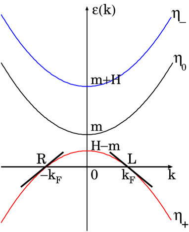
Figure 1: Spin-1 magnon band structure at $H>m$.

Take notice that the linearized dispersion and the definition of $L$ and $R$ become less reliable as the field $H$ becomes closer to the lower critical value $m$ ($v_{F}\to 0$).

So far we have omitted the inter-magnon interaction terms in this section. They would yield interactions among $L$, $R$, $\xi_{\nu}^{3}$ and $\eta_{-}$ (see the next section). A better method of dealing with such terms is the Abelian bosonization. Through it, the Dirac-fermion part in the effective theory (104) is mapped to the following Gaussian model,

$$\hat{\cal H}[L,R] \to \hat{\cal H}[\phi]=\int dx\,\frac{v}{2}\left[K(\partial_{x}\theta)^{2}+\frac{1}{K}(\partial_{x}\phi)^{2}\right],$$ (105)

where $\phi$ is a scalar field, $\theta$ is the dual of $\phi$, $v$ is the renormalized Fermi velocity, and $K$ is the TLL parameter: although $K=1$ and $v=v_{F}$ at the stage of Eq. (104), both parameters are subject to the renormalization due to irrelevant interaction effects neglected here. The Hamiltonian (105) just describes the low-energy physics of the TLL phase in the chain (4).

4 Field-theory representation of spin operators in $\boldsymbol{H}>\boldsymbol{m}$

Making use of the contents in the preceding sections, we construct a field-theory representation of spin operators in the uniform-field-induced TLL phase in the spin-1 AF chain (4).

4.1 Spin uniform component and Magnetization

First, we consider the uniform component of the spin, $\vec{J}=\vec{J}_{L}+\vec{J}_{R}$ in Eq. (7). In the low-energy limit, Eqs. (90) and (3) allow us to approximate the “old” Dirac fermion $\psi_{\nu}$ as follows:

$$\psi_{R}(x) \approx \frac{1}{\sqrt{2}}\eta_{-}(x)+e^{ik_{F}x}U_{+}L(x)+e^{-ik_{F}x}U_{-}R(x),$$

$$\psi_{L}(x) \approx \frac{i}{\sqrt{2}}\eta_{-}(x)-ie^{ik_{F}x}U_{-}L(x)-ie^{-ik_{F}x}U_{+}R(x),$$ (106)

where the prefactor $1[i]/\sqrt{2}$ of the first term is the $(1,1)$ $[(2,1)]$ component of the matrix ${\cal U}_{k=0}$, and $U_{\pm}=m/\sqrt{2H(H\pm\sqrt{H^{2}-m^{2}})}$ is the $(1,1)$ component of ${\cal U}_{\mp k_{F}}$. Note that $U_{\pm}$ have properties (i) $U_{\pm}\to 1/\sqrt{2}$ at $H\to m+0$, (ii) $U_{+}^{2}+U_{-}^{2}=1$, and (iii) $U_{+}U_{-}=\frac{m}{2H}$. From this relationship between $\psi_{\nu}$ and $(L,R,\eta_{-})$ [see also Eqs. (96)-(3)], we know how the latter three fields are transformed by symmetry operations. The U(1) rotation in Eq. (47) corresponds to

$$\eta_{-}\to e^{i\gamma}\eta_{-},\hskip 14.22636pt\left\{\begin{array}[]{cc}L\to e^{i\gamma}L\\ R\to e^{i\gamma}R\end{array}\right..$$ (109)

The one-site translation in Eq. (52) is mapped to

$$\eta_{-}(x)\to-\eta_{-}(x+a_{0}),\hskip 14.22636pt\left\{\begin{array}[]{cc}L(x)\to-e^{ik_{F}a_{0}}L(x+a_{0})\\ R(x)\to-e^{-ik_{F}a_{0}}R(x+a_{0})\end{array}\right..$$ (112)

The site-parity transformation in Eq. (73), $\psi_{L}(x)\to\mp\psi_{R}(-x)$ and $\psi_{R}(x)\to\pm\psi_{L}(-x)$, can be reproduced by

$$\eta_{-}(x)\to\pm i\eta_{-}(-x),\hskip 14.22636pt\left\{\begin{array}[]{cc}L(x)\to\mp iR(-x)\\ R(x)\to\mp iL(-x)\end{array}\right..$$ (115)

One can confirm that the Hamiltonian (104) is invariant under these transformations.

Using the relation (4.1), we can rewrite fields $\xi_{\nu}^{1,3}$ in $\vec{J}_{L,R}$ in terms of $L$, $R$, and $\eta_{-}$. As a result, the currents $\vec{J}_{L,R}$ are reexpressed as

$$J_{L}^{1}(x) \approx \Big{[}-\frac{i}{2}(\eta_{-}^{\dagger}+\eta_{-})+\frac{i}{\sqrt{2}}U_{-}(e^{-ik_{F}x}L^{\dagger}+e^{ik_{F}x}L)$$ (116a)

$$+\frac{i}{\sqrt{2}}U_{+}(e^{ik_{F}x}R^{\dagger}+e^{-ik_{F}x}R)\Big{]}\xi_{L}^{3},$$

$$J_{L}^{2}(x) \approx \Big{[}\frac{1}{2}(\eta_{-}^{\dagger}-\eta_{-})-\frac{1}{\sqrt{2}}U_{-}(e^{-ik_{F}x}L^{\dagger}-e^{ik_{F}x}L)$$ (116b)

$$-\frac{1}{\sqrt{2}}U_{+}(e^{ik_{F}x}R^{\dagger}-e^{-ik_{F}x}R)\Big{]}\xi_{L}^{3},$$

$$J_{L}^{3}(x) \approx \frac{1}{4}(\eta_{-}\eta_{-}^{\dagger}-\eta_{-}^{\dagger}\eta_{-})+\frac{U_{-}^{2}}{2}(LL^{\dagger}-L^{\dagger}L)+\frac{U_{+}^{2}}{2}(RR^{\dagger}-R^{\dagger}R)$$ (116c)

$$+\frac{U_{-}}{\sqrt{2}}\left[e^{ik_{F}x}\eta_{-}^{\dagger}L+{\rm h.c}\right]+\frac{U_{+}}{\sqrt{2}}\left[e^{-ik_{F}x}\eta_{-}^{\dagger}R+{\rm h.c}\right]$$

$$-U_{+}U_{-}\left[e^{-2ik_{F}x}L^{\dagger}R+{\rm h.c}\right],$$

$$J_{R}^{1}(x) \approx \Big{[}\frac{1}{2}(\eta_{-}^{\dagger}-\eta_{-})+\frac{1}{\sqrt{2}}U_{+}(e^{-ik_{F}x}L^{\dagger}-e^{ik_{F}x}L)$$ (116d)

$$+\frac{1}{\sqrt{2}}U_{-}(e^{ik_{F}x}R^{\dagger}-e^{-ik_{F}x}R)\Big{]}\xi_{R}^{3},$$

$$J_{R}^{2}(x) \approx \Big{[}\frac{i}{2}(\eta_{-}^{\dagger}+\eta_{-})+\frac{i}{\sqrt{2}}U_{+}(e^{-ik_{F}x}L^{\dagger}+e^{ik_{F}x}L)$$ (116e)

$$+\frac{i}{\sqrt{2}}U_{-}(e^{ik_{F}x}R^{\dagger}+e^{-ik_{F}x}R)\Big{]}\xi_{R}^{3},$$

$$J_{R}^{3}(x) \approx \frac{1}{4}(\eta_{-}\eta_{-}^{\dagger}-\eta_{-}^{\dagger}\eta_{-})+\frac{U_{+}^{2}}{2}(LL^{\dagger}-L^{\dagger}L)+\frac{U_{-}^{2}}{2}(RR^{\dagger}-R^{\dagger}R)$$ (116f)

$$-\frac{U_{+}}{\sqrt{2}}\left[e^{ik_{F}x}\eta_{-}^{\dagger}L+{\rm h.c}\right]-\frac{U_{-}}{\sqrt{2}}\left[e^{-ik_{F}x}\eta_{-}^{\dagger}R+{\rm h.c}\right]$$

$$-U_{+}U_{-}\left[e^{-2ik_{F}x}L^{\dagger}R+{\rm h.c}\right],$$

It is easily found that the above $\vec{J}_{L,R}$ are appropriately transformed for the symmetry operations (109), (47), (112), (52), (115) and (73). In addition, the Hermitian nature of all current operators is preserved in Eq. (47). Even if, instead of Eq. (4.1), we use precise representations of continuous fields in the Fourier space such as Eqs. (3) and (3), we can finally arrive at the same expression as Eq. (47).

The Fermi wave number $k_{F}$ is related with the uniform magnetization $M=\langle S_{j}^{z}\rangle$. It is given by the formula (47) or the Fourier-space representation of $J^{3}=J_{L}^{3}+J_{R}^{3}$. The result is

$$M = \frac{1}{N}\left\langle\sum_{j}S_{j}^{z}\right\rangle=\frac{1}{N}\int dx\,\langle J^{3}(x)\rangle$$ (116dm)

$$\left(\approx\frac{1}{N}\int dx\,\frac{1}{2}\left[\langle LL^{\dagger}-L^{\dagger}L\rangle+\langle RR^{\dagger}-R^{\dagger}R\rangle+\langle\eta_{-}\eta_{-}^{\dagger}\rangle\right]\right)$$

$$= \sum_{|k|<k_{F}}\langle\tilde{\eta}_{+}(k)\tilde{\eta}_{+}^{\dagger}(k)\rangle=\frac{k_{F}a_{0}}{\pi}.$$

From the derivation process of Eq. (116dm), we also find that the first three terms in Eqs. (116c) and (116f) should respectively be regarded as

$$\frac{1}{4}\left(\eta_{-}\eta_{-}^{\dagger}-\eta_{-}^{\dagger}\eta_{-}\right)+\frac{U_{-}^{2}}{2}\left(LL^{\dagger}-L^{\dagger}L\right)+\frac{U_{+}^{2}}{2}\left(RR^{\dagger}-R^{\dagger}R\right)$$

$$\,\,\,\,\to\,\,-U_{-}^{2}:L^{\dagger}L:-U_{+}^{2}:R^{\dagger}R:+\frac{M}{2a_{0}}-\frac{1}{2}\eta_{-}^{\dagger}\eta_{-},$$

$$\frac{1}{4}\left(\eta_{-}\eta_{-}^{\dagger}-\eta_{-}^{\dagger}\eta_{-}\right)+\frac{U_{+}^{2}}{2}\left(LL^{\dagger}-L^{\dagger}L\right)+\frac{U_{-}^{2}}{2}\left(RR^{\dagger}-R^{\dagger}R\right)$$

$$\,\,\,\,\to\,\,-U_{+}^{2}:L^{\dagger}L:-U_{-}^{2}:R^{\dagger}R:+\frac{M}{2a_{0}}-\frac{1}{2}\eta_{-}^{\dagger}\eta_{-}.$$ (116dn)

Utilizing the results (47) -(4.1), and applying the Abelian bosonization to the Dirac fermion $(L,R)$, we can straightforwardly lead to the following partially bosonized currents $\vec{J}_{L,R}$:

$$J_{L}^{1}(x) \approx \Big{[}-\frac{i}{2}(\eta_{-}^{\dagger}+\eta_{-})+\frac{iU_{-}}{\sqrt{\pi\alpha^{\prime}}}\kappa_{L}\cos(\sqrt{4\pi}\phi_{L}-\pi Mx/a_{0})$$

$$+\frac{iU_{+}}{\sqrt{\pi\alpha^{\prime}}}\kappa_{R}\cos(\sqrt{4\pi}\phi_{R}-\pi Mx/a_{0})\Big{]}\xi_{L}^{3},$$

$$J_{L}^{2}(x) \approx \Big{[}\frac{1}{2}(\eta_{-}^{\dagger}-\eta_{-})-\frac{iU_{-}}{\sqrt{\pi\alpha^{\prime}}}\kappa_{L}\sin(\sqrt{4\pi}\phi_{L}-\pi Mx/a_{0})$$

$$+\frac{iU_{+}}{\sqrt{\pi\alpha^{\prime}}}\kappa_{R}\sin(\sqrt{4\pi}\phi_{R}-\pi Mx/a_{0})\Big{]}\xi_{L}^{3},$$

$$J_{L}^{3}(x) \approx -\frac{U_{-}^{2}}{\sqrt{\pi}}\,\partial_{x}\phi_{L}-\frac{U_{+}^{2}}{\sqrt{\pi}}\,\partial_{x}\phi_{R}+\frac{M}{2a_{0}}-\frac{1}{2}\eta_{-}^{\dagger}\eta_{-}$$

$$+\frac{U_{-}}{\sqrt{4\pi\alpha^{\prime}}}\left[\eta_{-}^{\dagger}\kappa_{L}e^{-i\sqrt{4\pi}\phi_{L}+i\pi Mx/a_{0}}+{\rm h.c}\right]$$

$$+\frac{U_{+}}{\sqrt{4\pi\alpha^{\prime}}}\left[\eta_{-}^{\dagger}\kappa_{R}e^{i\sqrt{4\pi}\phi_{R}-i\pi Mx/a_{0}}+{\rm h.c}\right]$$

$$-i\frac{U_{+}U_{-}}{\pi\alpha^{\prime}}\kappa_{L}\kappa_{R}\sin(\sqrt{4\pi}\phi-2\pi Mx/a_{0}),$$

$$J_{R}^{1}(x) \approx \Big{[}\frac{1}{2}(\eta_{-}^{\dagger}-\eta_{-})+\frac{iU_{+}}{\sqrt{\pi\alpha^{\prime}}}\kappa_{L}\sin(\sqrt{4\pi}\phi_{L}-\pi Mx/a_{0})$$

$$-\frac{iU_{-}}{\sqrt{\pi\alpha^{\prime}}}\kappa_{R}\sin(\sqrt{4\pi}\phi_{R}-\pi Mx/a_{0})\Big{]}\xi_{R}^{3},$$

$$J_{R}^{2}(x) \approx \Big{[}\frac{i}{2}(\eta_{-}^{\dagger}+\eta_{-})+\frac{iU_{+}}{\sqrt{\pi\alpha^{\prime}}}\kappa_{L}\cos(\sqrt{4\pi}\phi_{L}-\pi Mx/a_{0})$$

$$+\frac{iU_{-}}{\sqrt{\pi\alpha^{\prime}}}\kappa_{R}\cos(\sqrt{4\pi}\phi_{R}-\pi Mx/a_{0})\Big{]}\xi_{R}^{3},$$

$$J_{R}^{3}(x) \approx -\frac{U_{+}^{2}}{\sqrt{\pi}}\,\partial_{x}\phi_{L}-\frac{U_{-}^{2}}{\sqrt{\pi}}\,\partial_{x}\phi_{R}+\frac{M}{2a_{0}}-\frac{1}{2}\eta_{-}^{\dagger}\eta_{-}$$ (116do)

$$-\frac{U_{+}}{\sqrt{4\pi\alpha^{\prime}}}\left[\eta_{-}^{\dagger}\kappa_{L}e^{-i\sqrt{4\pi}\phi_{L}+i\pi Mx/a_{0}}+{\rm h.c}\right]$$

$$-\frac{U_{-}}{\sqrt{4\pi\alpha^{\prime}}}\left[\eta_{-}^{\dagger}\kappa_{R}e^{i\sqrt{4\pi}\phi_{R}-i\pi Mx/a_{0}}+{\rm h.c}\right]$$

$$-i\frac{U_{+}U_{-}}{\pi\alpha^{\prime}}\kappa_{L}\kappa_{R}\sin(\sqrt{4\pi}\phi-2\pi Mx/a_{0}),$$

where $\alpha^{\prime}\sim 1/\Lambda^{\prime}$ is the short-distance cut off, and $\kappa_{L(R)}$ is the Klein factor for the field $L(R)$. Therefore, the bosonized uniform components of the spin are written as

$$J^{3}(x) \approx \frac{M}{a_{0}}-\frac{1}{\sqrt{\pi}}\partial_{x}\phi-\eta_{-}^{\dagger}\eta_{-}-iC_{0}^{z}\kappa_{L}\kappa_{R}\sin(\sqrt{4\pi}\phi-2\pi Mx/a_{0})$$ (116dpa)

$$+C_{1}^{z}\left(\eta_{-}^{\dagger}\kappa_{L}e^{-i\sqrt{\pi}(\phi+\theta)+i\pi Mx/a_{0}}+{\rm h.c}\right)$$

$$-C_{1}^{z}\left(\eta_{-}^{\dagger}\kappa_{R}e^{-i\sqrt{\pi}(\phi-\theta)-i\pi Mx/a_{0}}+{\rm h.c}\right)+\cdots,$$

$$J^{+}(x) \equiv J^{1}(x)+iJ^{2}(x)$$ (116dpb)

$$\approx \bigg{\{}-i\eta_{-}+e^{-i\sqrt{\pi}\theta}\Big{[}iC_{1}\kappa_{L}e^{-i\sqrt{\pi}\phi+\pi Mx/a_{0}}$$

$$+iC_{2}\kappa_{R}e^{i\sqrt{\pi}\phi-\pi Mx/a_{0}}+\cdots\Big{]}+\cdots\bigg{\}}\xi_{L}^{3}$$

$$+\bigg{\{}-\eta_{-}-e^{-i\sqrt{\pi}\theta}\Big{[}C_{2}\kappa_{L}e^{-i\sqrt{\pi}\phi+\pi Mx/a_{0}}$$

$$+C_{1}\kappa_{R}e^{i\sqrt{\pi}\phi-\pi Mx/a_{0}}+\cdots\Big{]}+\cdots\bigg{\}}\xi_{R}^{3},$$

where $C_{n}$ and $C_{n}^{z}$ are nonuniversal constants, which contain the effects of irrelevant terms neglected at the stage (104). When the irrelevant terms are not taken into account, constants $C_{0}^{z}$, $C_{1}^{z}$, $C_{1}$, and $C_{2}$ are respectively proportional to $U_{+}U_{-}$, $U_{-}-U_{+}$, $U_{-}$, and $U_{+}$. Therefore, it is inferred that $C_{1}^{z}\to 0$ at $H\to m+0$. In Eqs. (4.1) and (51), we used the formula (116dpdrdseaebecexeyezfjflfv). If, instead of it, we use another formula (A), we can add more irrelevant terms to Eqs. (4.1) and (51). Namely, we may perform the replacement,

$$e^{\pm i\sqrt{\pi}(\phi+\theta)\mp i\pi Mx/a_{0}} \to \sum_{n=0}^{\infty}\tilde{C}_{n}e^{\pm i(2n+1)(\sqrt{\pi}\phi-\pi Mx/a_{0})}e^{\pm i\sqrt{\pi}\theta},$$

$$e^{\pm i\sqrt{\pi}(\phi-\theta)\mp i\pi Mx/a_{0}} \to \sum_{n=0}^{\infty}\tilde{C}_{n}e^{\pm i(2n+1)(\sqrt{\pi}\phi-\pi Mx/a_{0})}e^{\mp i\sqrt{\pi}\theta},$$ (116dpdq)

where $\tilde{C}_{n}$ is a nonuniversal constant. Equation (51) is a main result in this paper. We expect that replacing the Klein factors in Eq. (51) with a constant is admitted in most situations. (A typical situation is when one investigates asymptotic features of spin correlation functions. See Sec. 4.4.)

Finally, using the results (47)-(4.1), let us investigate how the current-current interaction $\lambda$ term modifies the parameter $K$ of the effective theory (105). Since the SU(2) spin-rotation symmetry is reduced to the U(1) one in the case with a finite $H$, the term $-\lambda\vec{J}_{L}\vec{J}_{R}$ might be modified to $-\lambda_{\perp}(J_{L}^{1}J_{R}^{1}+J_{L}^{2}J_{R}^{2})-\lambda_{\parallel}J_{L}^{3}J_{R}^{3}$, in which we assume that both $\lambda_{\perp}$ and $\lambda_{\parallel}$ are positive. Equations (47) and (4.1) lead to the following representation of the current-current interaction [52]:

$$J_{L}^{3}(x_{+})J_{R}^{3}(x) \approx \left(U_{-}^{2}:R^{\dagger}R:+U_{+}^{2}:L^{\dagger}L:\right)\left(U_{+}^{2}:R^{\dagger}R:+U_{-}^{2}:L^{\dagger}L:\right)$$ (116dpdra)

$$+U_{+}^{2}U_{-}^{2}\left(L^{\dagger}R(x_{+})R^{\dagger}L(x)+R^{\dagger}L(x_{+})L^{\dagger}R(x)\right)$$

$$-\frac{M}{2a_{0}}\left(:L^{\dagger}L:+:R^{\dagger}R:\right)$$

$$+\frac{U_{+}^{2}+U_{-}^{2}}{2}\eta_{-}^{\dagger}\eta_{-}\left(:L^{\dagger}L:+:R^{\dagger}R:\right)$$

$$-\frac{U_{+}U_{-}}{2}\left[\eta_{-}^{\dagger}\eta_{-}(L(x_{+})L^{\dagger}(x)+R(x_{+})R^{\dagger}(x))+{\rm h.c.}\right]$$

$$+\frac{U_{-}^{2}-U_{+}^{2}}{2}\left(\eta_{-}^{\dagger}(x_{+})\eta_{-}^{\dagger}(x)LR+{\rm h.c.}\right)$$

$$+\,\,\,{\rm oscillating\,\,terms}\,\,\,+\,\,\,{\rm others},$$

$$J_{L}^{1}(x_{+})J_{R}^{1}(x)+J_{L}^{2}(x_{+})J_{R}^{2}(x)\approx$$

$$\hskip 85.35826ptiU_{+}U_{-}\left(L^{\dagger}L-LL^{\dagger}+R^{\dagger}R-RR^{\dagger}\right)\xi_{L}^{3}\xi_{R}^{3}$$

$$\hskip 85.35826pt+\,\,\,{\rm oscillating\,\,terms}\,\,\,+\,\,\,{\rm others},$$ (116dpdrb)

where we used $x_{+}=x+\delta$ ($\delta$ is a small parameter of ${\cal O}(a_{0})$), “oscillating terms” have a factor $e^{\pm in\pi Mx/a_{0}}$ ($n$: integer), which are irrelevant except for the case that $M$ is close to a special commensurate value, and “others” are constructed by only massive fields $(\xi_{\nu}^{3},\eta_{-})$. The Hamiltonian (104) plus the above current-current interaction is regarded as a more accurate low-energy effective theory for the uniform-field-driven TLL phase. Integrating out the part of massive fields $(\xi_{\nu}^{3},\eta_{-})$ in the effective theory [53], we obtain a Hamiltonian for the interacting Dirac fermion $(L,R)$ that just corresponds to the Gaussian theory (105). In the Gaussian theory framework, the first and second terms of Eq. (116dpdra) directly contribute to the renormalization of the TLL parameter $K$ and the velocity $v$ as follows. The bosonized forms of these two terms are written as

$$\left(U_{-}^{2}:R^{\dagger}R:+U_{+}^{2}:L^{\dagger}L:\right)\left(U_{+}^{2}:R^{\dagger}R:+U_{-}^{2}:L^{\dagger}L:\right)$$

$$\hskip 19.91684pt\to\frac{1}{4\pi}(\partial_{x}\phi)^{2}-\frac{(U_{-}^{2}-U_{+}^{2})^{2}}{4\pi}(\partial_{x}\theta)^{2}$$

$$\hskip 28.45274pt+\frac{U_{-}^{4}-U_{+}^{4}}{4\pi}\left[\partial_{x}\phi\partial_{x}\theta-\partial_{x}\theta\partial_{x}\phi\right],$$ (116dpdrdsa)

$$U_{+}^{2}U_{-}^{2}\left(L^{\dagger}R(x_{+})R^{\dagger}L(x)+R^{\dagger}L(x_{+})L^{\dagger}R(x)\right)$$

$$\hskip 19.91684pt\to\frac{U_{+}^{2}U_{-}^{2}}{(2\pi\alpha^{\prime})^{2}}\left[e^{i\sqrt{4\pi}(\phi(x_{+})-\phi(x))}+e^{-i\sqrt{4\pi}(\phi(x_{+})-\phi(x))}\right]$$

$$\hskip 19.91684pt\approx-\frac{m^{2}}{4\pi H^{2}}\left(\partial_{x}\phi\right)^{2}+{\rm const}+\cdots,$$ (116dpdrdsb)

where we used $U_{+}^{2}+U_{-}^{2}=1$ and $U_{+}U_{-}=\frac{m}{2H}$, and assumed $\delta=\alpha^{\prime}$. The final term in Eq. (116dpdrdsa) could be negligible or be replaced with a constant: such a procedure is supported by the equal-time commutation relation $[\phi(x),\theta(y)]=-\frac{i}{2}{\rm sgn}(x-y)$. Consequently, two terms in Eq. (54) lead to an additional boson kinetic term,

$$-\frac{1}{4\pi}(\lambda_{\parallel}-\frac{m^{2}}{H^{2}}\lambda_{\perp})(\partial_{x}\phi)^{2}+\frac{\lambda_{\parallel}}{4\pi}(U_{-}^{2}-U_{+}^{2})^{2}(\partial_{x}\theta)^{2},$$ (116dpdrdsdt)

for the $K=1$ Gaussian theory (105) [54]. This term is inclined to make the parameter $K$ increase, i.e., $K>1$, provided that $\lambda_{\parallel}$ is the same order as $\lambda_{\perp}$. The relation $K>1$ is consistent with the predictions of the numerical calculation in Ref. [25] and the NLSM approach [24]. (It is shown in Ref. [25] that $K$ is between 1.0 and 1.5 in the field-induced TLL state.) Besides Eq. (54), other terms in Eq. (53) also yields a correction of $K$ and $v$, but it is expected that the property $K>1$ is maintained. From Eq. (53), one also finds that the current-current interaction does not generate any relevant or marginal vertex operators such as $\cos(\sqrt{4\pi}\phi)$. It means that the massless TLL phase survives even when the $\lambda$ interaction is taken into account. The third normal-ordered term in Eq. (116dpdra) provides only a small correction of the magnetization $M$, and can be absorbed into the Gaussian theory via $\phi(x)\to\phi(x)-{\rm const}\times x$.

4.2 Spin staggered component

Compared with the formula (51) for the uniform component of the spin, the way of leading to a field-theory formula for the staggered component $\vec{N}(x)$ is not straightforward, because we have to express the vertex operators $e^{\pm i\sqrt{\pi}\Theta}$ and $e^{\pm i\sqrt{\pi}\Phi}$ in Eq. (2.3) in terms of another boson $(\phi,\theta)$ language and the magnon $\eta_{-}$ one. To this end, we apply the discussion in Ref. [29].

First, using some results in the previous sections, let us naively speculate the relation between the “old” boson $(\Phi,\Theta)$ and the “new” one $(\phi,\theta)$. The expression of $J^{3}(x)$ in Eqs. (2.3) and (116dpa) indicates the following relation between $\Phi$ and $\phi$,

$$-\frac{1}{\sqrt{\pi}}\partial_{x}\Phi(x) \approx -\frac{1}{\sqrt{\pi}}\partial_{x}\phi(x)+M/a_{0}$$ (116dpdrdsdu)

$$-iC_{0}^{z}\kappa_{L}\kappa_{R}\,\sin(\sqrt{4\pi}\phi-2\pi Mx/a_{0})+\cdots.$$

Performing the integration with respect to $x$ in Eq. (116dpdrdsdu), we obtain

$$\Phi(x) \approx \phi(x)-\sqrt{\pi}Mx/a_{0}+\cdots,$$ (116dpdrdsdv)

where we dropped the sin term because it oscillates and then vanishes in the integration. From this, we can expect that

$$e^{\pm i\sqrt{\pi}\Phi} \sim e^{\pm i(\sqrt{\pi}\phi-\pi Mx/a_{0})},$$ (116dpdrdsdw)

holds within a rough approximation. We next consider dual fields $\Theta$ and $\theta$. The U(1) spin rotation in Eq. (109) could be realized by

$$\theta(x) \to \theta(x)-\frac{\gamma}{\sqrt{\pi}},$$ (116dpdrdsdx)

in the boson language. The comparison between this and Eq. (47) implies the relation,

$$e^{\pm i\sqrt{\pi}\Theta} \sim e^{\pm i\sqrt{\pi}\theta}.$$ (116dpdrdsdy)

In order to raise the validity of speculations (116dpdrdsdw) and (116dpdrdsdy), and obtain a more appropriate relationship between $e^{\pm i\sqrt{\pi}\Phi(\Theta)}$ and $(\phi,\theta,\eta_{-})$, a standard bosonization formula,

$$\psi_{L}=\frac{\zeta_{L}}{\sqrt{2\pi\alpha}}e^{-i\sqrt{\pi}(\Phi+\Theta)},\hskip 14.22636pt\psi_{R}=\frac{\zeta_{R}}{\sqrt{2\pi\alpha}}e^{i\sqrt{\pi}(\Phi-\Theta)},$$ (116dpdrdsdz)

is available. From this formula, we rewrite vertex operators $e^{-i\sqrt{\pi}\Phi}$ and $e^{-i\sqrt{\pi}\Theta}$ as

$$e^{-i\sqrt{\pi}\Phi} = \sqrt{2\pi\alpha}\left[{\cal D}e^{i\sqrt{\pi}\Theta}\zeta_{L}\psi_{L}+(1-{\cal D})e^{-i\sqrt{\pi}\Theta}\zeta_{R}\psi_{R}^{\dagger}\right],$$ (116dpdrdseaa)

$$e^{-i\sqrt{\pi}\Theta} = \sqrt{2\pi\alpha}\left[{\cal D}e^{i\sqrt{\pi}\Phi}\zeta_{L}\psi_{L}+(1-{\cal D})e^{-i\sqrt{\pi}\Phi}\zeta_{R}\psi_{R}\right],$$ (116dpdrdseab)

where $\cal D$ is an arbitrary constant [55]. Then, employing approximated results (116dpdrdsdw), (116dpdrdsdy), (4.1), and the bosonization formula $L,R\sim e^{\mp i\sqrt{4\pi}\phi_{L,R}}$ in the right-hand sides in Eq. (62), we can arrive at a desirable representation of $e^{\pm i\sqrt{\pi}\Phi(\Theta)}$. This method was proposed in Ref. [29].

Following the above idea, we obtain

$$e^{-i\sqrt{\pi}\Theta} \approx \sqrt{\frac{\alpha}{4\alpha^{\prime}}}e^{-i\sqrt{\pi}\theta}\bigg{[}U_{-}\left(-i\zeta_{L}\kappa_{L}+\zeta_{R}\kappa_{R}\right)$$ (116dpdrdseaeba)

$$+U_{+}\left(-i\zeta_{L}\kappa_{R}e^{i\sqrt{4\pi}\phi-2\pi Mx/a_{0}}+\zeta_{R}\kappa_{L}e^{-i\sqrt{4\pi}\phi+2\pi Mx/a_{0}}\right)\bigg{]}$$

$$+\frac{\sqrt{\pi\alpha}}{2}\left(i\zeta_{L}e^{i\sqrt{\pi}\phi-\pi Mx/a_{0}}+\zeta_{R}e^{-i\sqrt{\pi}\phi+\pi Mx/a_{0}}\right)\eta_{-}$$

$$+\cdots,$$

$$e^{-i\sqrt{\pi}\Phi} \approx \sqrt{\frac{\alpha}{4\alpha^{\prime}}}\bigg{[}U_{-}\left(-i\zeta_{L}\kappa_{L}+\zeta_{R}\kappa_{R}\right)e^{-i\sqrt{\pi}\phi+\pi Mx/a_{0}}$$ (116dpdrdseaebb)

$$+U_{+}\left(-i\zeta_{L}\kappa_{R}+\zeta_{R}\kappa_{L}\right)e^{i\sqrt{\pi}\phi-\pi Mx/a_{0}}\bigg{]}$$

$$+\frac{\sqrt{\pi\alpha}}{2}\left(i\zeta_{L}\eta_{-}e^{i\sqrt{\pi}\theta}+\zeta_{R}\eta_{-}^{\dagger}e^{-i\sqrt{\pi}\theta}\right)+\cdots,$$

where we set ${\cal D}=1/2$, and $\kappa_{L(R)}$ is the Klein factor of the field $L(R)$ [56]. It is found that the naive expectations (116dpdrdsdw) and (116dpdrdsdy) are qualitatively consistent with the result (63). From this formula, our target, the staggered component of the spin may be represented as

$$N^{3}(x) = \sigma^{3}\cos(\sqrt{\pi}\Phi)$$ (116dpdrdseaebeca)

$$\approx \sigma^{3}\bigg{[}D_{1}^{z}\cos\left(\sqrt{\pi}\phi-\pi Mx/a_{0}\right)$$

$$+{D_{1}^{z}}^{\prime}\left\{(i\zeta_{L}+\zeta_{R})\eta_{-}e^{i\sqrt{\pi}\theta}+{\rm h.c.}\right\}\bigg{]}+\cdots,$$

$$N^{+}(x) \equiv N^{1}(x)+iN^{2}(x)=i\mu^{3}e^{-i\sqrt{\pi}\Theta}$$ (116dpdrdseaebecb)

$$\approx \mu^{3}e^{-i\sqrt{\pi}\theta}\bigg{[}D_{1}+D_{2}\cos\left(\sqrt{4\pi}\phi-2\pi Mx/a_{0}\right)+\cdots\bigg{]}$$

$$+D^{\prime}_{1}\mu^{3}\left(i\zeta_{L}e^{i\sqrt{\pi}\phi-\pi Mx/a_{0}}+\zeta_{R}e^{-i\sqrt{\pi}\phi+\pi Mx/a_{0}}\right)\eta_{-}$$

$$+\cdots,$$

where $D_{n}^{(z,\prime)}$ are nonuniversal constants, which include effects of irrelevant terms, and we naively omitted some of Klein factors $\zeta_{\nu}$ and $\kappa_{\nu}$. We used the formula $L,R\sim e^{\mp i\sqrt{4\pi}\phi_{L,R}}$ in Eqs. (63) and (64). Instead of that, applying the formula (A), we can introduce more irrelevant terms in Eqs. (63) and (64) [see the replacement (4.1)]. For instance, we might replace $\cos(\sqrt{\pi}\phi-\pi Mx/a_{0})$ in Eq. (116dpdrdseaebeca) with

$$\sum_{n=0}^{\infty}\tilde{D}_{n}\cos\left[(2n+1)(\sqrt{\pi}\phi-\pi Mx/a_{0})\right],$$ (116dpdrdseaebeced)

where $\tilde{D}_{n}$ is a nonuniversal constant.

4.3 Symmetries

Through several considerations, we obtained a field-theory formula for spin operators, Eqs. (51) and (64). Using the formula, transformations (109)-(115) and the effective Hamiltonians (104) and (105), we can consider how the symmetries of the spin-1 AF chain (4) are represented in the partially-bosonized effective theory framework.

(i) As we discussed already, a U(1) rotation around the spin z axis, $S_{j}^{+}\to e^{i\gamma}S_{j}^{+}$, could be realized by

$$\eta_{-}\to e^{i\gamma}\eta_{-},\hskip 28.45274pt\theta\to\theta-\frac{\gamma}{\sqrt{\pi}}.$$ (116dpdrdseaebecee)

(ii) The one-site translation $\vec{S}_{j}\to\vec{S}_{j+1}$ may correspond to

$$\eta_{-}(x)\to-\eta_{-}(x+a_{0}),\hskip 14.22636pt\xi_{L,R}^{3}(x)\to-\xi_{L,R}^{3}(x+a_{0}),$$

$$\left\{\begin{array}[]{ccc}\theta(x)\to\theta(x+a_{0})+\sqrt{\pi}\\ \phi(x)\to\phi(x+a_{0})-\sqrt{\pi}M\end{array}\right.,\hskip 14.22636pt\left\{\begin{array}[]{ccc}\sigma^{3}(x)\to-\sigma^{3}(x+a_{0})\\ \mu^{3}(x)\to\mu^{3}(x+a_{0})\end{array}\right..$$ (116dpdrdseaebecej)

These transformations cooperatively change the staggered factor $(-1)^{j}$ in front of $\vec{N}(x)$ into $(-1)^{j+1}$.

(iii) The site-parity transformation $\vec{S}_{j}\to\vec{S}_{-j}$ might be regarded as [51]

$$\eta_{-}(x)\to\pm i\eta_{-}(-x),\hskip 14.22636pt\left\{\begin{array}[]{ccc}\xi_{L}^{3}(x)\to\mp\xi_{R}^{3}(-x)\\ \xi_{R}^{3}(x)\to\pm\xi_{L}^{3}(-x)\end{array}\right.,$$ (116dpdrdseaebecem)

$$\left\{\begin{array}[]{ccc}\kappa_{L}\to\mp i\kappa_{R}\\ \kappa_{R}\to\mp i\kappa_{L}\\ \phi(x)\to-\phi(-x)\\ \theta(x)\to\theta(-x)\end{array}\right.,\hskip 5.69046pt\left\{\begin{array}[]{ccc}\sigma^{3}(x)\to\sigma^{3}(-x)\\ \mu^{3}(x)\to\mu^{3}(-x)\end{array}\right.,\hskip 5.69046pt\left\{\begin{array}[]{ccc}\zeta_{L}\to\mp\zeta_{R}\\ \zeta_{R}\to\pm\zeta_{L}\end{array}\right..$$ (116dpdrdseaebecev)

These symmetry operations might tell us which additional terms are allowed to be present in formulas (51) and (64): for example, the staggered component $N^{3}(x)$ may include $\sigma^{3}(\{(i\zeta_{L}+\zeta_{R})\partial_{x}\eta_{-}\}^{n}e^{in\sqrt{\pi}\theta}+{\rm h.c.})$, $\sigma^{3}\eta_{-}^{\dagger}\eta_{-}$, etc ($n$: an integer). These terms are properly transformed for all the symmetry operations.

If we integrate out massive fields in the partition function and replace all massive-field parts in spin operators with their expectation values, the effective Hamiltonian becomes the Gaussian model (105) and the reduced spin operators containing only massless boson fields are given by

$$J^{3}(x) \to \frac{M}{a_{0}}-\frac{1}{\sqrt{\pi}}\partial_{x}\phi+C_{0}^{z}\cos\left(\sqrt{4\pi}\phi-2\pi Mx/a_{0}\right)+\cdots,$$

$$N^{+}(x) \to e^{-i\sqrt{\pi}\theta}\langle\mu^{3}\rangle\left[D_{1}+D_{2}\cos\left(\sqrt{4\pi}\phi-2\pi Mx/a_{0}\right)+\cdots\right],$$

$$(J^{+}(x))^{2} \to e^{-2i\sqrt{\pi}\theta}\Big{[}{\bar{C}}_{1}+{\bar{C}}_{2}\cos\left(\sqrt{4\pi}\phi-2\pi Mx/a_{0}\right)+\cdots\Big{]},$$

$$(N^{3}(x))^{2} \to {\bar{D}}_{1}+{\bar{D}}_{2}\cos\left(\sqrt{4\pi}\phi-2\pi Mx/a_{0}\right)+\cdots,$$ (116dpdrdseaebecew)

where ${\bar{C}}_{n}$ and ${\bar{D}}_{n}$ are nonuniversal constants, all the Klein factors are naively eliminated, and we used $(\sigma^{3}(x))^{2}\sim{\rm const}$, $\langle\eta_{-}\eta_{-}^{\dagger}\rangle\sim{\cal O}(a_{0}^{-1})$, and $\langle\xi_{\nu}^{3}\xi_{\nu^{\prime}}^{3}\rangle\sim{\cal O}(a_{0}^{-1})$ (see  B). This result indicates that the compactification radius of $\phi$ and that of $\theta$ are respectively $1/\sqrt{4\pi}$ and $1/\sqrt{\pi}$. In this bosonized-theory framework, we could interpret that the U(1) rotation $S_{j}^{+}\to e^{i\gamma}S_{j}^{+}$, the one-site translation $\vec{S}_{j}\to\vec{S}_{j+1}$, and the site-parity operation $\vec{S}_{j}\to\vec{S}_{-j}$, respectively, corresponds to

$$\theta\to\theta-\frac{\gamma}{\sqrt{\pi}},$$ (116dpdrdseaebecexa)

$$\theta(x)\to\theta(x+a_{0})+\sqrt{\pi},\hskip 28.45274pt\phi(x)\to\phi(x+a_{0})-\sqrt{\pi}M,$$ (116dpdrdseaebecexb)

$$\phi(x)\to-\phi(-x),\hskip 28.45274pt\theta(x)\to\theta(-x).$$ (116dpdrdseaebecexc)

The symmetries of Eq. (70) strongly restrict the emergence of the relevant vertex operators in the effective field theory (105): the U(1) symmetry (116dpdrdseaebecexa) [the translational symmetry (116dpdrdseaebecexb)] forbids $e^{in\sqrt{\pi}\theta}$ [$e^{in\sqrt{4\pi}\phi}$] to exist in the effective Hamiltonian [57]. Consequently, the TLL state stably remains.

One can see that the above transformations (70) are very similar to those of the effective bosonization theory for spin-1/2 AF chains (see C).

4.4 Asymptotic behavior of spin correlation functions

Applying the formulas (51) and (64), let us investigate equal-time spin correlation functions in the field-induced TLL phase. The asymptotic forms of equal-time two-point functions of $\vec{J}$ and $\vec{N}$ are evaluated as

$$\langle J^{3}(x)J^{3}(0)\rangle \approx \left(\frac{M}{a_{0}}\right)^{2}+\frac{1}{\pi}\langle\partial_{x}\phi(x)\partial_{x}\phi(0)\rangle$$ (116dpdrdseaebecexeya)

$$+{\cal A}^{z}\cos\left(2\pi M\frac{x}{a_{0}}\right)\langle e^{-i\sqrt{4\pi}\phi(x)}e^{i\sqrt{4\pi}\phi(0)}\rangle+\cdots$$

$$= \left(\frac{M}{a_{0}}\right)^{2}-\frac{K}{2\pi^{2}}\frac{1}{x^{2}}$$

$$+{\cal A}^{z}\cos\left(2\pi M\frac{x}{a_{0}}\right)\left(\frac{\alpha^{\prime}}{x}\right)^{2K}+\cdots,$$

$$\langle J^{+}(x)J^{-}(0)\rangle \approx {\cal A}\cos\left(\pi M\frac{x}{a_{0}}\right)\langle e^{-i\sqrt{\pi}(\phi\pm\theta)(x)}e^{i\sqrt{\pi}(\phi\pm\theta)(0)}\rangle$$ (116dpdrdseaebecexeyb)

$$\times\langle\xi_{L/R}^{3}(x)\xi_{L/R}^{3}(0)\rangle+\cdots$$

$$\sim \cos\left(\pi M\frac{x}{a_{0}}\right)\left(\frac{\alpha^{\prime}}{x}\right)^{\frac{K+K^{-1}}{2}}K_{1}\left(\frac{x}{\xi_{c}}\right)+\cdots,$$

$$\langle N^{3}(x)N^{3}(0)\rangle \approx {\cal B}^{z}\cos\left(\pi M\frac{x}{a_{0}}\right)\langle\sigma^{3}(x)\sigma^{3}(0)\rangle$$ (116dpdrdseaebecexeyc)

$$\times\langle e^{-i\sqrt{\pi}\phi(x)}e^{i\sqrt{\pi}\phi(0)}\rangle+\cdots$$

$$\sim \cos\left(\pi M\frac{x}{a_{0}}\right)\left(\frac{\alpha^{\prime}}{x}\right)^{K/2}K_{0}\left(\frac{x}{\xi_{c}}\right)+\cdots,$$

$$\langle N^{+}(x)N^{-}(0)\rangle \approx {\cal B}_{1}\langle\mu^{3}(x)\mu^{3}(0)\rangle\langle e^{-i\sqrt{\pi}\theta(x)}e^{i\sqrt{\pi}\theta(0)}\rangle\Big{[}1$$ (116dpdrdseaebecexeyd)

$$+{\cal B}_{2}\cos\left(2\pi M\frac{x}{a_{0}}\right)\langle e^{-i\sqrt{4\pi}\phi(x)}e^{i\sqrt{4\pi}\phi(0)}\rangle+\cdots\Big{]}$$

$$\sim \left(\frac{\alpha^{\prime}}{x}\right)^{1/(2K)}+{\cal B}_{2}^{\prime}\cos\left(2\pi M\frac{x}{a_{0}}\right)$$

$$\times\left(\frac{\alpha^{\prime}}{x}\right)^{\frac{1}{2K}+2K}+\cdots,$$

where ${\cal A}^{(z)}$ and ${\cal B}^{(z,\prime)}_{(n)}$ are nonuniversal constants, $K_{\nu}$ is the modified Bessel function, and $x\gg\xi_{c}(=v_{0}/m)$. In the calculation of Eq. (71), we used Eqs. (2.1) [see the comment [48]], (A), (116dpdrdseaebecexeyezfjflgd)-(B). From this result, longitudinal and transverse spin-spin correlators are determined as

$$\langle S_{j}^{z}S_{0}^{z}\rangle \approx M^{2}-\frac{K}{2\pi^{2}}\left(\frac{a_{0}}{x}\right)^{2}+{\cal C}_{0}^{z}\cos\left(2\pi Mj\right)\left(\frac{a_{0}}{x}\right)^{2K}$$ (116dpdrdseaebecexeyeza)

$$+{\cal D}_{1}^{z}\cos\left(\pi(1+M)j\right)\left(\frac{a_{0}}{x}\right)^{(K+1)/2}e^{-x/\xi_{c}}+\cdots,$$

$$\langle S_{j}^{+}S_{0}^{-}\rangle \approx {\cal C}_{1}\cos\left(\pi Mj\right)\left(\frac{a_{0}}{x}\right)^{(K+K^{-1}+1)/2}e^{-x/\xi_{c}}$$ (116dpdrdseaebecexeyezb)

$$+{\cal D}_{1}(-1)^{j}\left(\frac{a_{0}}{x}\right)^{1/(2K)}$$

$$+{\cal D}_{2}\cos\left(\pi(1+2M)j\right)\left(\frac{a_{0}}{x}\right)^{\frac{1}{2K}+2K}+\cdots,$$

where $x=ja_{0}\gg\xi_{c}$, and ${\cal C}_{q}^{(z)}$ and ${\cal D}_{q}^{(z)}$ are nonuniversal constants which are related to $C_{n}^{(z)}$ and $D_{n}^{(z,\prime)}$ in Eqs. (51) and (64). The first two terms in $\langle S_{j}^{z}S_{0}^{z}\rangle$ and the second term in $\langle S_{j}^{+}S_{0}^{-}\rangle$ can also be derived by the NLSM plus Ginzbrug-Landau approach [23, 24], but it is difficult to obtain all the other terms within the same approach. One can verify that the critical exponent of the incommensurate part around wave number $p\sim\pm 2k_{F}$ ($k_{F}=\pi M/a_{0}$) in $\langle S_{j}^{z}S_{0}^{z}\rangle$, $\eta_{z}=2K$, and that of the staggered part in $\langle S_{j}^{+}S_{0}^{-}\rangle$, $\eta=1/(2K)$, satisfy the famous relation $\eta\eta_{z}=1$ [58, 59, 23, 29, 10]. In addition, it is found that the contribution around $p\sim\pi/a_{0}\pm k_{F}$ in $\langle S_{j}^{z}S_{0}^{z}\rangle$ and that around $p\sim\pm k_{F}$ in $\langle S_{j}^{+}S_{0}^{-}\rangle$ exhibit an exponential decay. Comparing Eq. (72) with the spin correlators of a two-leg spin-1/2 ladder in a uniform field in Ref. [29] would be instructive (although our calculations in Eqs. (71) and (72) are rougher than those in Ref. [29]). Besides Eq. (72), using the formulas (51) and (64), one can calculate various physical quantities (susceptibilities, dynamical structure factors, NMR relaxation rates, etc) in the TLL phase [24].

In all the calculations of this subsection, we assumed that the three systems $\hat{\cal H}[\phi]$, $\hat{\cal H}[\xi^{3}]$, and $\hat{\cal H}[\eta_{-}]$ are independent of each other. Although small interactions among these systems would actually be present, it is expected that their effects in the low-energy, long-distance physics are almost negligible and could be absorbed into some parameters such as $K$, $v_{(0)}$, $m$, etc.

5 Some applications of the field-theory representation of spin operators

In this section, utilizing the derived formulas (51) and (64), we discuss some topics for the low-energy physics in/around the uniform-field-induced TLL phase.

5.1 String order parameter

As a quantity characterizing the Haldane phase ($H<m$), there is the nonlocal string order parameter which can detect the so-called “hidden AF long-range order” in the phase [60, 61, 8]. It is defined by

$$O_{\alpha}(i,j) = -\lim_{|i-j|\to\infty}\left\langle S_{i}^{\alpha}\exp\left(i\pi\sum_{n=i+1}^{j-1}S_{n}^{\alpha}\right)S_{j}^{\alpha}\right\rangle.$$ (116dpdrdseaebecexeyezfa)

In the continuous-field-theory framework, we can predict [41, 40] that the string parameter is approximated as follows:

$$O_{\alpha}(i,j) \sim \langle\mu^{\alpha+1}(x_{i})\mu^{\alpha+2}(x_{i})\mu^{\alpha+1}(x_{j})\mu^{\alpha+2}(x_{j})\rangle,$$ (116dpdrdseaebecexeyezfb)

where $x_{i}=ia_{0}$ and $x_{j}=ja_{0}$. Actually, the right-hand side is a finite, non-zero value in the Haldane phase where $\langle\mu^{\alpha}\rangle\neq 0$.

From the formula (A), the z component of the string parameter is rewritten as

$$O_{z}(i,j) \sim \langle\cos(\sqrt{\pi}\Phi(x_{i}))\cos(\sqrt{\pi}\Phi(x_{j}))\rangle.$$ (116dpdrdseaebecexeyezfc)

In the field-induced TLL phase ($H>m$), the vertex operator $\exp(\pm i\sqrt{\pi}\Phi)$ is represented by using fields $(\phi,\theta,\eta_{-})$ [see Eqs. (116dpdrdseaebb) and (116dpdrdseaebeca)]. Hence, it is predicted that in the TLL phase, $O_{z}(i,j)$ behaves as

$$O_{z}(i,j) \sim \langle\cos(\sqrt{\pi}\phi(x_{i})-\pi Mi)\cos(\sqrt{\pi}\phi(x_{j})-\pi Mj)\rangle+\cdots$$ (116dpdrdseaebecexeyezfd)

$$\sim \cos\left[\pi M(i-j)\right]\left(\frac{a_{0}}{x_{i}-x_{j}}\right)^{K/2}+\cdots.$$

Namely, $O_{z}(i,j)$ is shown to exhibit power decay in the TLL phase.

5.2 SU(2)-invariant perturbations

In Secs. 5.2-5.4, we investigate typical perturbations for the critical TLL state. In particular, we focus on whether or not the perturbation terms yield a first excitation gap, and the symmetries of them.

In this subsection, we discuss two terms: the bond alternation $\sum_{j}(-1)^{j}J\delta\vec{S}_{j}\cdot\vec{S}_{j+1}$ ($|\delta|\ll 1$) and the next-nearest-neighbor (NNN) exchange $\sum_{j}J_{2}\vec{S}_{j}\cdot\vec{S}_{j+2}$ ($|J_{2}|\ll J$), which are invariant under the global SU(2) transformation. Because a global U(1) symmetry, a part of the SU(2) one, is usually necessary for the realization of the TLL i.e., a $c=1$ CFT [1, 2, 4, 8], and (as we mentioned in Sec. 4.3) it prohibits all vertex operators with the dual field $\theta(x)$ from emerging in the effective Hamiltonian, we expect, without any calculations, that the TLL phase survives even when these perturbations are applied. Let us consider the two terms below in more detail.

From the continuous-field formula (7), we can expect that the bond alternation term is approximated as

$$\sum_{j}(-1)^{j}J\delta\vec{S}_{j}\cdot\vec{S}_{j+1}=\sum_{j}J\delta(-1)^{j}\left[\frac{1}{2}\left(S_{j}^{+}S_{j+1}^{-}+{\rm h.c}\right)+S_{j}^{z}S_{j+1}^{z}\right]$$

$$\sim J\delta a_{0}\int dx\bigg{\{}(-1)^{j}\Big{[}\frac{1}{2}\left(J^{+}(x)J^{-}(x+a_{0})+{\rm h.c}\right)+J^{z}(x)J^{z}(x+a_{0})$$

$$-\frac{1}{2}\left(N^{+}(x)N^{-}(x+a_{0})+{\rm h.c}\right)+N^{z}(x)N^{z}(x+a_{0})\Big{]}$$

$$+\frac{1}{2}\left(-J^{+}(x)N^{-}(x+a_{0})+N^{+}(x)J^{-}(x+a_{0})+{\rm h.c}\right)$$

$$-J^{z}(x)N^{z}(x+a_{0})+N^{z}(x)J^{z}(x+a_{0})\bigg{\}}.$$ (116dpdrdseaebecexeyezfe)

Let us substitute the formulas (51) and (64) into the above result, although such a procedure sometimes causes mistakes (see the comment [55]). As a result, we obtain

$$\sum_{j}(-1)^{j}J\delta\vec{S}_{j}\cdot\vec{S}_{j+1} \to J\delta\int dx\sum_{n=1}^{\infty}\Big{[}\lambda_{n}^{\prime}\cos(n(\sqrt{4\pi}\phi-2\pi Mj)+\alpha_{n}^{\prime})$$ (116dpdrdseaebecexeyezff)

$$+(-1)^{j}\lambda_{n}\cos(n(\sqrt{4\pi}\phi-2\pi Mj)+\alpha_{n})\Big{]}$$

$$+\cdots,$$

where $\lambda_{n}^{(\prime)}$ and $\alpha_{n}^{(\prime)}$ are nonuniversal constants. Here, we used $(\sigma^{3}(x))^{2}\sim{\rm const}$, and the operator product expansion (OPE) $\mu^{3}\times\xi_{L,R}^{3}\sim\sigma^{3}+\cdots$ [1, 2, 4, 62], and then integrated out all the massive-field parts in the partition function (see the comment [53]). In order to more restrict the form of Eq. (116dpdrdseaebecexeyezff), we utilize the symmetry argument. For the one-site translation and the site-parity operation, the bond alternation term changes its sign. Its bosonized form should also have the same property; namely, we require the right-hand side in Eq. (116dpdrdseaebecexeyezff) to change the sign for $\phi(x)\to\phi(x+a_{0})-\sqrt{\pi}M$ and $\phi(x)\to-\phi(-x)$ [see Eq. (70)]. Consequently, we set $\lambda_{n}^{\prime}=0$ and $\alpha_{n}=\pi/2$. The resultant form of Eq. (116dpdrdseaebecexeyezff) is

$$\sum_{j}(-1)^{j}J\delta\vec{S}_{j}\cdot\vec{S}_{j+1} \to J\delta\int dx\sum_{n=1}^{\infty}(-1)^{j}\lambda_{n}\sin(n(\sqrt{4\pi}\phi-2\pi Mj))$$ (116dpdrdseaebecexeyezfg)

$$+\cdots.$$

This bosonized form indicates that in general, the bond alternation is irrelevant in the TLL phase due to the staggered factor $(-1)^{j}$ and the phase $2n\pi Mj$. However, when $M=1/2$ (half of the saturation), a relevant interaction $\sin(\sqrt{4\pi}\phi)$ originates from the $n=1$ term in Eq. (116dpdrdseaebecexeyezfg) because of the cancellation of two factors $(-1)^{j}$ and $2\pi Mj$. The scaling dimension $\Delta_{s}$ of $\sin(\sqrt{4\pi}\phi)$ is $K$ ($1\leq K<1.5$ [25]). At this case of $M=1/2$, the low-energy physics may be described by a sine-Gordon theory, and an infinitesimal bond alternation induces a finite excitation gap and a finite dimerization parameter $\langle\vec{S}_{2n}\cdot\vec{S}_{2n+1}-\vec{S}_{2n+1}\cdot\vec{S}_{2n+2}\rangle$. The existence of the gap further means that the bond alternation brings an $M=1/2$ plateau in the uniform magnetization process. The scaling argument near a criticality [63] shows that the bond-alternation-induced gap $\Delta_{\delta}$ and dimerization parameter respectively behave as

$$\Delta_{\delta}\sim|\delta|^{1/(2-K)},$$

$$\langle\vec{S}_{2n}\cdot\vec{S}_{2n+1}-\vec{S}_{2n+1}\cdot\vec{S}_{2n+2}\rangle\sim-{\rm sgn}(\delta)|\delta|^{K/(2-K)},$$ (116dpdrdseaebecexeyezfh)

for a small $|\delta|$. Because of the inequality $1/(2-K)>1$, the gap gradually grows with increasing $|\delta|$. These predictions for the (small) bond alternation are consistent with previous numerical [64] and analytical [65] works.

Next, let us tern to the NNN coupling ($J_{2}$) term. Through an argument similar to that above, we arrive in the following result:

$$\sum_{j}J_{2}\vec{S}_{j}\cdot\vec{S}_{j+2} \to J_{2}\int dx\Big{\{}\frac{a_{0}}{\pi}(\partial_{x}\phi)^{2}-\frac{2M}{\sqrt{\pi}}\partial_{x}\phi$$ (116dpdrdseaebecexeyezfi)

$$+\sum_{n=1}^{\infty}\tilde{\lambda}_{n}\cos(n(\sqrt{4\pi}\phi-2\pi Mj))+\cdots\Big{\}},$$

where $\tilde{\lambda}_{n}$ is a nonuniversal constant. We used the symmetry argument: the right-hand side in Eq. (116dpdrdseaebecexeyezfi) is invariant under $\phi(x)\to\phi(x+a_{0})-\sqrt{\pi}M$ and $\phi(x)\to-\phi(-x)$. Since the bosonized NNN coupling does not contain any relevant operators for arbitrary magnetization values, we conclude that the TLL phase remains even when a sufficiently small NNN exchange perturbation is introduced. The derivative term $\partial_{x}\phi$ is absorbed into the Gaussian part via $\phi\to\phi-{\rm const}J_{2}\times x$ and provides a small correction of the magnetization $M$. While the boson quadratic term $(\partial_{x}\phi)^{2}$ makes the velocity $v$ and the TLL parameter $K$ modify. After easy calculations, we can see that when $J_{2}>0$ ($J_{2}<0$), $M$ and $K$ decrease (increase), but $v$ increases (decreases).

5.3 Axially symmetric terms

In this subsection, we consider three kinds of U(1)-symmetric perturbation terms: the single-ion anisotropy $D_{z}\sum_{j}(S_{j}^{z})^{2}$ (so-called $D$ term), the XXZ type anisotropy $J\Delta_{z}\sum_{j}S_{j}^{z}S_{j+1}^{z}$, and the staggered-field Zeeman term along the spin z axis $-h_{z}\sum_{j}(-1)^{j}S_{j}^{z}$ ($|D_{z}|,|h_{z}|\ll J$ and $|\Delta_{z}|\ll 1$). As in the cases of the bond alternation and the NNN coupling, there is a high possibility that the TLL phase survives as these perturbations are added.

Following the similar argument to that in the last subsection, we can bosonize the three terms as follows:

$$D_{z}\sum_{j}(S_{j}^{z})^{2} \to D_{z}\int dx\Big{\{}\frac{a_{0}}{\pi}(\partial_{x}\phi)^{2}-\frac{2M}{\sqrt{\pi}}\partial_{x}\phi$$ (116dpdrdseaebecexeyezfja)

$$+\sum_{n=1}^{\infty}d_{n}\cos(n(\sqrt{4\pi}\phi-2\pi Mj))+\cdots\Big{\}},$$

$$J\Delta_{z}\sum_{j}S_{j}^{z}S_{j+1}^{z} \to J\Delta_{z}\int dx\Big{\{}\frac{a_{0}}{\pi}(\partial_{x}\phi)^{2}-\frac{2M}{\sqrt{\pi}}\partial_{x}\phi$$ (116dpdrdseaebecexeyezfjb)

$$+\sum_{n=1}^{\infty}\delta_{n}\cos(n(\sqrt{4\pi}\phi-2\pi Mj))+\cdots\Big{\}},$$

$$-h_{z}\sum_{j}(-1)^{j}S_{j}^{z} \to -h_{z}\int dx\Big{\{}(-1)^{j}\sum_{n=1}^{\infty}z_{n}\cos(n(\sqrt{4\pi}\phi-2\pi Mj))$$ (116dpdrdseaebecexeyezfjc)

$$+\cdots\Big{\}},$$

where $d_{n}$, $\delta_{n}$ and $z_{n}$ are nonuniversal constants. For instance, we required the bosonization form (116dpdrdseaebecexeyezfjc) of the staggered-field term to change its sign for the one-site translation $\phi(x)\to\phi(x+a_{0})-\sqrt{\pi}M$ and to be invariant under the site-parity transformation $\phi(x)\to-\phi(-x)$. The results (116dpdrdseaebecexeyezfja) and (116dpdrdseaebecexeyezfjb) suggest that the $D$ term and the XXZ exchange play almost the same roles in the low-energy, long-distance physics of the TLL phase. If $D_{z}>0$ ($D_{z}<0$), $M$ and $K$ decrease (increase), while $v$ increases (decreases). As expected, these three terms generally do not destroy the TLL state. However, as in the case of the bond alternation term, when the uniform magnetization $M$ becomes close to 1/2, the staggered-field term involves a relevant term $\cos(\sqrt{4\pi}\phi)$ with $\Delta_{s}=K$. Therefore, a staggered-field-induced gap $\Delta_{h_{z}}$ opens and $\langle S_{j}^{z}\rangle$ obtains a staggered component at $M=1/2$. From the standard scaling argument, the gap and the magnetization are shown to behave as

$$\Delta_{h_{z}} \sim |h_{z}|^{1/(2-K)},$$

$$\langle S_{j}^{z}\rangle \approx \frac{1}{2}+(-1)^{j}f\left(\frac{H}{J}\right){\rm sgn}(h_{z})|h_{z}|^{K/(2-K)},$$ (116dpdrdseaebecexeyezfjfk)

where $f$ is a function.

5.4 Axial-symmetry-breaking terms

Here, we discuss three axial-symmetry-breaking terms: the $D$ term with the x component of spin $D_{x}\sum_{j}(S_{j}^{x})^{2}$, another kind of the single-ion anisotropy (so-called $E$ term) $E\sum_{j}[(S_{j}^{x})^{2}-(S_{j}^{y})^{2}]=\frac{E}{2}\sum_{j}[(S_{j}^{+})^{2}+(S_{j}^{-})^{2}]$, and the staggered-field term along the spin x axis $-h_{x}\sum_{j}(-1)^{j}S_{j}^{x}$ ($|D_{x}|,|E|,|h_{x}|\ll J$). Since the three terms destroy the axial U(1) symmetry ($\theta\to\theta-\gamma/\sqrt{\pi}$), vertex operators with $\theta(x)$ are allowed to be present in the effective Hamiltonian. It is inferred that such vertex operators cause an instability of the TLL state, and then a finite excitation gap occurs. Here, note that the $D_{x}$ and $E$ terms are invariant under the $\pi$ rotation $S^{+}_{j}\to-S^{+}_{j}$ ($\theta\to\theta-\sqrt{\pi}$) [20], whereas the $h_{x}$ term obtains a minus sign via the same rotation. Furthermore, the $\pi/2$ rotation leaves the $E$ term change the sign.

Through some calculations, the three perturbation terms are bosonized as

$$D_{x}\sum_{j}(S_{j}^{x})^{2} \to D_{x}\int dx\Big{\{}\cos(\sqrt{4\pi}\theta)\sum_{n=0}^{\infty}d_{n}^{(1)}\cos(n(\sqrt{4\pi}\phi-2\pi Mj))$$ (116dpdrdseaebecexeyezfjfla)

$$+\cos(4\sqrt{\pi}\theta)\sum_{n=0}^{\infty}d_{n}^{(2)}\cos(n(\sqrt{4\pi}\phi-2\pi Mj))$$

$$+\sum_{n=0}^{\infty}d_{n}^{(3)}\cos(n(\sqrt{4\pi}\phi-2\pi Mj))+\cdots\Big{\}},$$

$$E\sum_{j}[(S_{j}^{x})^{2}-(S_{j}^{y})^{2}] \to E\int dx\Big{\{}\cos(\sqrt{4\pi}\theta)\times$$ (116dpdrdseaebecexeyezfjflb)

$$\sum_{n=0}^{\infty}e_{n}\cos(n(\sqrt{4\pi}\phi-2\pi Mj))+\cdots\Big{\}},$$

$$-h_{x}\sum_{j}(-1)^{j}S_{j}^{x} \to -h_{x}\int dx\Big{\{}\cos(\sqrt{\pi}\theta)$$ (116dpdrdseaebecexeyezfjflc)

$$\times\sum_{n=0}^{\infty}x_{n}\cos(n(\sqrt{4\pi}\phi-2\pi Mj))+\cdots\Big{\}},$$

where $d_{n}^{(l)}$, $e_{n}$ and $x_{n}$ are nonuniversal constants. (Since the bosonized form of the anisotropic exchange $J\Delta_{x}\sum_{j}S_{j}^{x}S_{j+1}^{x}$ is the same type as Eq. (116dpdrdseaebecexeyezfjfla), we do not discuss it here.) One should note the following properties: (i) $\cos(\sqrt{\pi}\theta)\to-\cos(\sqrt{\pi}\theta)$, $\cos(\sqrt{4\pi}\theta)\to\cos(\sqrt{4\pi}\theta)$ and $\cos(4\sqrt{\pi}\theta)\to\cos(4\sqrt{\pi}\theta)$ for the $\pi$ rotation, and (ii) $\cos(\sqrt{4\pi}\theta)\to-\cos(\sqrt{4\pi}\theta)$ for the $\pi/2$ rotation.

The most relevant operator in both $D_{x}$ and $E$ terms is always $\cos(\sqrt{4\pi}\theta)$ with $\Delta_{s}=1/K<2$. Thus, the low-energy properties can be explained by a sine-Gordon model, and a gap emerges. Supposing $d_{0}^{(1)}$ and $e_{0}$ are positive, the potential $\cos(\sqrt{4\pi}\theta)$ pins the phase field $\theta$ to $\pm\sqrt{\pi}/2$ ($0$ or $\sqrt{\pi}$) modulo $2\sqrt{\pi}$ for $D_{x},E>0$ ($D_{x},E<0$). In such a case of $\theta\to\pm\sqrt{\pi}/2$ ($\to 0$ or $\sqrt{\pi}$), it is expected that $\langle S^{x}_{j}\rangle\sim(-1)^{j}\langle\cos(\sqrt{\pi}\theta)\rangle=0$ ($\neq 0$) and $\langle S^{y}_{j}\rangle\sim(-1)^{j}\langle\sin(\sqrt{\pi}\theta)\rangle\neq 0$ ($=0$). From this prediction and the scaling argument [$\Delta_{s}$ of $e^{i\sqrt{\pi}\theta}$ is $1/(4K)$], we conclude that for a small $D_{x}$ term, the gap $\Delta_{D_{x}}$ and the transverse component of the spin moment increase as follows:

$$\Delta_{D_{x}}\sim|D_{x}|^{K/(2K-1)},$$

$$\left\{\begin{array}[]{ccc}\langle S^{x}_{j}\rangle&\sim&0\\ \langle S^{y}_{j}\rangle&\sim&(-1)^{j}{D_{x}}^{1/(8K-4)}\end{array}\right.,\hskip 14.22636pt({\rm for}\,\,D_{x}>0),$$ (116dpdrdseaebecexeyezfjflfo)

$$\left\{\begin{array}[]{ccc}\langle S^{x}_{j}\rangle&\sim&(-1)^{j}|D_{x}|^{1/(8K-4)}\\ \langle S^{y}_{j}\rangle&\sim&0\end{array}\right.,\hskip 14.22636pt({\rm for}\,\,D_{x}<0).$$ (116dpdrdseaebecexeyezfjflfr)

Of course, for a small $E$ term, the similar results hold: we may replace $D_{x}$ to $E$ in Eq. (5.4). The staggered moment (i.e., a Néel order) along the spin x or y axis shows that the $D_{x}$ (or $E$) term causes the spontaneous breakdown of the one-site translational symmetry. Because of $K/(2K-1)<1$ and $1/(8K-4)<1$, the $D_{x}$- or $E$-term-induced gap and the transverse moment $\langle S^{x,y}_{j}\rangle$ rapidly increases with the growth of $|D_{x}|$ or $|E|$.

The staggered-field $h_{x}$ term contains the relevant term $\cos(\sqrt{\pi}\theta)$ with $\Delta_{s}=1/(4K)<2$. Therefore, the $h_{x}$-induced gap $\Delta_{h_{x}}$ and the staggered magnetization are shown to behave as

$$\Delta_{h_{x}}\sim|h_{x}|^{4K/(8K-1)},\hskip 14.22636pt\langle S^{x}_{j}\rangle\sim(-1)^{j}{\rm sgn}(h_{x})|h_{x}|^{1/(8K-1)}.$$ (116dpdrdseaebecexeyezfjflfs)

For the spin-1/2 AF Heisenberg chain, which low-energy sector is also described by a TLL theory (see Introduction), a staggered field also yields a gap and a staggered moment. Oshikawa and Affleck [66] show that in the spin-1/2 case, $\Delta_{h_{x}}\sim|h_{x}|^{2/3}$ and $\langle S^{x}_{j}\rangle\sim(-1)^{j}{\rm sgn}(h_{x})|h_{x}|^{1/3}$. The result (116dpdrdseaebecexeyezfjflfs) thus indicates that the growth of both the gap and the staggered moment in the spin-1 case is much sharper than that in the spin-1/2 case.

5.5 Magnon decay induced by axial-symmetry-breaking terms

In this subsection, we briefly mention the magnon-decay processes, which have already in some detail discussed in Ref. [20]. In order to consider such processes, let us go back to the effective Hamiltonian (95), where $\tilde{\eta}_{+}$, $\tilde{\eta}_{0}^{\dagger}$ and $\tilde{\eta}_{-}^{\dagger}$ respectively denote the $S^{z}=+1$, $0$ and $-1$ magnon creation operators. The marginally irrelevant $\lambda$ term, omitted in Eq. (95), just contribute to the magnon decay.

First, we focus on the U(1)-symmetric AF chain (4) without any perturbations. Since the one-magnon excitations are present only around $p=\pi/a_{0}$, only the decay from a magnon to an odd number of magnons is possible. If $H$ is increased so that $3\epsilon_{+}(0)<\epsilon_{-}(0)$ ($H>m/2$) [$3\epsilon_{+}(0)<\epsilon_{0}(0)$ ($H>2m/3$)] are satisfied, a magnon $\tilde{\eta}_{-}^{\dagger}$ [$\tilde{\eta}_{0}^{\dagger}$] is energetically permitted to decay into three magnons $\tilde{\eta}_{+}\tilde{\eta}_{+}\tilde{\eta}_{+}$ via the $\lambda$ term. However, since $\tilde{\eta}_{+}$, $\tilde{\eta}_{0}^{\dagger}$ and $\tilde{\eta}_{-}^{\dagger}$ possess different eigenvalues of $S^{z}$ (namely, three kinds of one-magnon states are in different sectors of the Hilbert space), this type of the decay is forbidden. Indeed, for a U(1) rotation $S_{j}^{+}\to e^{i\gamma}S_{j}^{+}$, $\tilde{\eta}_{-}$ [$\tilde{\eta}_{0}$] is transformed as $\tilde{\eta}_{-}\to e^{i\gamma}\tilde{\eta}_{-}$ [$\tilde{\eta}_{0}\to\tilde{\eta}_{0}$ (invariant)], while the product $\tilde{\eta}_{+}\tilde{\eta}_{+}\tilde{\eta}_{+}$ obey a different rotation $\tilde{\eta}_{+}\tilde{\eta}_{+}\tilde{\eta}_{+}\to e^{3i\gamma}\tilde{\eta}_{+}\tilde{\eta}_{+}\tilde{\eta}_{+}$. Three kinds of magnons ($\tilde{\eta}_{+}$, $\tilde{\eta}_{0}^{\dagger}$, $\tilde{\eta}_{-}^{\dagger}$) therefore would be well-defined quasiparticles in the U(1)-symmetric system (4).

On the other hand, when a U(1)-symmetry-breaking term is introduced, there is a possibility that the above decay processes are allowed. In the case with the $D_{x}$ or $E$ terms, the $\pi$-rotation symmetry ($S_{j}^{+}\to-S_{j}^{+}$: $\gamma=\pi$), a part of the U(1) rotation, survives. For this rotation, $\tilde{\eta}_{-}$ and $\tilde{\eta}_{+}\tilde{\eta}_{+}\tilde{\eta}_{+}$ are odd, whereas $\tilde{\eta}_{0}$ is even. Furthermore, from Eqs. (99) and (3), we find that for example a sum of four terms “$\tilde{\eta}_{-}(k_{1})\tilde{\eta}_{+}(k_{2})\tilde{\eta}_{+}(-k_{1})\tilde{\eta}_{+}(-k_{2})-(k_{1,2}\to-k_{1,2})+{\rm h.c}$” is invariant under both the one-site translation and the site-parity operation. (Because the site-parity operation (3) is the result of the approximation, the requirement of the invariance under this transformation might be too strong.) As a result, the process $\tilde{\eta}_{-}^{\dagger}\to\tilde{\eta}_{+}\tilde{\eta}_{+}\tilde{\eta}_{+}$ is permissible. It is hence inferred that as sufficiently strong $D_{x}$ or $E$ terms are present in the system, $\tilde{\eta}_{-}^{\dagger}$ magnons become ill-defined particles, and we should eliminate the magnon fields from the Hamiltonian (104) and the field-theory formulas of the spin, Eqs. (51) and (64). In the case with the $h_{x}$ staggered-field term, symmetries of the $\pi$ rotation and the one-site translation are also broken (the two-site translational symmetry remains). Therefore, the magnon decay would be more promoted. When $H$ is further increased and the $\tilde{\eta}_{+}$-magnon condensation occurs ($H>m$), other types of the magnon decay are energetically admitted: for instance, $\tilde{\eta}_{-}^{\dagger}\to\tilde{\eta}_{0}^{\dagger}\tilde{\eta}_{0}^{\dagger}\tilde{\eta}_{+}\tilde{\eta}_{+}\tilde{\eta}_{+}$.

From the simple discussion above, one sees that as $H$ is sufficiently strong, a large axial-symmetry-breaking perturbation tends to make the lifetime of massive magnons shorten. However, if such a perturbation is small enough, our effective theory framework would still be reliable and have the ability to explain various low-energy properties of spin-1 AF chains.

6 Summary

In this paper, based on the Majorana fermion theory, we have reconsidered the field theory description of the spin-1 AF chain (4), and derived an explicit field-theory form of spin operators in the uniform-field-driven TLL phase in the chain (4), i.e., Eqs. (51) and (64) [the corresponding effective Hamiltonian is Eqs. (104) and (105)]. From the formula, we have completely determined the asymptotic forms of spin correlation functions (Sec. 4.4). Furthermore, applying the formula, we have investigated the string order parameter and effects of some perturbation terms (the bond alternation, the next-nearest interaction, anisotropy terms) in Sec. 5. We have estimated the excitation gaps and some physical quantities (staggered moments and the dimerization parameter) generated from the perturbations. From Sec. 2 to Sec. 5, we have often argued how symmetries of the spin-1 AF chain are represented in the effective field theory world.

Our results, especially Eqs. (51) and (64), must be useful in analyzing and understanding various spin-1 AF chains with magnons condensed (i.e., with a finite magnetization) and the extended models of them (e.g., spin-1 AF ladders, spatially anisotropic 2D or 3D spin-1 AF systems). The results of Sec. 5 guarantee this expectation. We will apply the contents of this paper to other spin-1 AF systems in the near future.

Determining nonuniversal coefficients in Eqs. (51), (64) and (4.3), especially those in front of terms including only massless bosons, is important for more quantitative predictions of (quasi) 1D spin-1 systems. A powerful way of the determination is to accurately evaluate the long-distance behavior of spin correlation functions by means of a numerical method such as DMRG and QMC [10].

Appendix A Abelian bosonization for fermion systems

Here, we briefly summarize the Abelian bosonization. As mentioned in Sec. 2, in (1+1)D case, a massless Dirac (complex) fermion or two species of massless Majorana (real) fermions (critical Ising models) are equivalent to a massless bosonic Gaussian theory. The former Hamiltonian is written as

$$\hat{\cal H}[\psi] = \int\,\,dx\,\,ic\left(\psi_{L}^{\dagger}\partial_{x}\psi_{L}-\psi_{R}^{\dagger}\partial_{x}\psi_{R}\right)$$ (116dpdrdseaebecexeyezfjflft)

$$= \int\,dx\,\,\sum_{q=1,2}\frac{i}{2}c\left(\xi_{L}^{q}\partial_{x}\xi_{L}^{q}-\xi_{R}^{q}\partial_{x}\xi_{R}^{q}\right)=\hat{\cal H}[\xi^{1},\xi^{2}],$$

where $\psi_{\nu}$ and $\xi_{\nu}^{q}$ are respectively the chiral components of the Dirac fermion and the real one, and $c$ is the Fermi velocity. These fermions obey anticommutation relations: $\{\xi_{\nu}^{q}(x),\xi_{\nu^{\prime}}^{q^{\prime}}(y)\}=\delta_{\nu,\nu^{\prime}}\delta_{q,q^{\prime}}\delta(x-y)$, $\{\psi_{\nu}(x),\psi_{\nu^{\prime}}(y)\}=0$ and $\{\psi_{\nu}(x),\psi_{\nu^{\prime}}^{\dagger}(y)\}=\delta_{\nu,\nu^{\prime}}\delta(x-y)$. The corresponding Hamiltonian of the Gaussian theory is

$$\hat{\cal H}[\phi] = \int\,dx\,\frac{c}{2}\left[(\partial_{x}\theta)^{2}+(\partial_{x}\phi)^{2}\right]=\int\,dx\,c\left[(\partial_{x}\phi_{L})^{2}+(\partial_{x}\phi_{R})^{2}\right],$$

where $\phi=\phi_{L}+\phi_{R}$ is the real scalar field, $\theta=\phi_{L}-\phi_{R}$ is the dual field of $\phi$, and $\phi_{L(R)}$ is the left (right) moving part of $\phi$. The fields $\phi$ and $\theta$ satisfy the canonical commutation relation $[\phi(x),\theta(y)]=-\frac{i}{2}{\rm sgn}(x-y)$. Chiral fields $\phi_{L,R}$ obey $[\phi_{L}(x),\phi_{R}(y)]=0$ and $[\phi_{L/R}(x),\phi_{L/R}(y)]=\mp\frac{i}{4}{\rm sgn}(x-y)$. In condensed-matter physics, the Hamiltonian (116dpdrdseaebecexeyezfjflft) usually originates from a microscopic system in solids (e.g., a lattice system such as the Hubbard chain and the Heisenberg one) after a coarse-graining or a renormalization procedure.

Among these fermion and boson fields, operator identities hold. The fermion annihilation (or creation) operators are bosonized as

$$\psi_{L}=\frac{\kappa_{L}}{\sqrt{2\pi\alpha}}\exp(-i\sqrt{4\pi}\phi_{L}),\hskip 14.22636pt\psi_{R}=\frac{\kappa_{R}}{\sqrt{2\pi\alpha}}\exp(i\sqrt{4\pi}\phi_{R}),$$ (116dpdrdseaebecexeyezfjflfv)

where $\kappa_{L,R}$ are Klein factors which satisfy $\{\kappa_{\nu},\kappa_{\nu^{\prime}}\}=2\delta_{\nu,\nu^{\prime}}$, and are necessary for the boson vertex (exponential) operators to reproduce the correct anticommutation relation between $\psi_{L}$ and $\psi_{R}$. The parameter $\alpha$ is a short-distance cut off, which depends on details of the microscopic model considered. (Note that it is possible to construct another formula without Klein factors, although it requires a modification of commutation relations among bosons. See Refs. [67, 68].) Following Haldane’s harmonic-fluid approach [69, 3, 10], one can obtain an alternative bosonized form of $\psi_{L}$ and $\psi_{R}$: when a real-space fermion field $\psi(x)$ in the considering microscopic system is approximated as $\psi\sim e^{ik_{F}x}\psi_{R}+e^{-ik_{F}x}\psi_{L}$, one may bosonize $\psi_{L,R}$ as

$$e^{-ik_{F}x}\psi_{L}=\frac{\kappa_{L}}{\sqrt{2\pi\alpha}}\sum_{n=0}^{\infty}e^{-i(2n+1)(\sqrt{\pi}\phi+k_{F}x)}e^{-i\sqrt{\pi}\theta},$$

$$e^{ik_{F}x}\psi_{R}=\frac{\kappa_{R}}{\sqrt{2\pi\alpha}}\sum_{n=0}^{\infty}e^{i(2n+1)(\sqrt{\pi}\phi+k_{F}x)}e^{-i\sqrt{\pi}\theta}.$$ (116dpdrdseaebecexeyezfjflfw)

The quantity $k_{F}$ is the Fermi wave number in the microscopic system. The $n=0$ most relevant terms correspond to Eq. (116dpdrdseaebecexeyezfjflfv). The chiral U(1) currents ${\cal J}_{L}=:\psi_{L}^{\dagger}\psi_{L}:$ and ${\cal J}_{R}=:\psi_{R}^{\dagger}\psi_{R}:$ are written as

$${\cal J}_{L}=\frac{1}{\sqrt{\pi}}\partial_{x}\phi_{L},\hskip 28.45274pt{\cal J}_{R}=\frac{1}{\sqrt{\pi}}\partial_{x}\phi_{R}.$$ (116dpdrdseaebecexeyezfjflfx)

In addition to the correspondences between the fermion and the boson, it is known [1, 4, 28, 29, 62, 70] that the Ising order and disorder fields $\sigma_{\nu}$ and $\mu_{\nu}$ can be bosonized as [71]

$$\sigma_{1}\sigma_{2}\sim\sin(\sqrt{\pi}\phi),\hskip 28.45274pt\mu_{1}\mu_{2}\sim\cos(\sqrt{\pi}\phi),$$

$$\sigma_{1}\mu_{2}\sim\cos(\sqrt{\pi}\theta),\hskip 28.45274pt\mu_{1}\sigma_{2}\sim\sin(\sqrt{\pi}\theta).$$ (116dpdrdseaebecexeyezfjflfy)

Following these Abelian bosonization rules, one can bosonize 1D interacting Dirac fermion systems as well as the free massless fermion (116dpdrdseaebecexeyezfjflft). If the interaction terms are all irrelevant in the sense of the renormalization group, the effective Hamiltonian at the low-energy limit is still a Gaussian type with the velocity $c$ and coefficients of $(\partial_{x}\phi)^{2}$ and $(\partial_{x}\theta)^{2}$ renormalized. Conventionally [3], the resultant Hamiltonian is written as

$$\hat{\cal H}^{\rm eff}[\phi] = \int dx\frac{c^{\prime}}{2}\left[{g}(\partial_{x}{\theta})^{2}+\frac{1}{g}(\partial_{x}{\phi})^{2}\right],$$ (116dpdrdseaebecexeyezfjflfz)

where $c^{\prime}$ is the renormalized velocity, and $g$ is called the TLL parameter (the Hamiltonian (A) corresponds to a $g=1$ theory). When a system is reduced to this type at the low-energy limit, we say that the system belongs to the TLL universality [69, 1, 2, 3]. The Gaussian theory [1, 2, 3, 4, 8] yields

$$\langle\partial_{x}\phi(x)\partial_{x}\phi(0)\rangle=-\frac{K}{2\pi}\frac{1}{x^{2}},$$

$$\langle e^{iq\sqrt{\pi}\phi(x)}e^{-iq^{\prime}\sqrt{\pi}\phi(0)}\rangle\sim\delta_{q,q^{\prime}}\left(\frac{\alpha}{x}\right)^{q^{2}g/2},$$

$$\langle e^{iq\sqrt{\pi}\theta(x)}e^{-iq^{\prime}\sqrt{\pi}\theta(0)}\rangle\sim\delta_{q,q^{\prime}}\left(\frac{\alpha}{x}\right)^{q^{2}/(2g)},$$ (116dpdrdseaebecexeyezfjflga)

where $q$ and $q^{\prime}$ are an integer (note the comment [50]). This result shows that the scaling dimensions of $\partial_{x}\phi$, $e^{iq\sqrt{\pi}\phi}$ and $e^{iq\sqrt{\pi}\theta}$ are respectively $1$, $q^{2}g/4$ and $q^{2}/(4g)$.

Appendix B Correlation functions of massive fermion theories

In this Appendix, we evaluate correlation functions of two massive fermion systems,

$$\hat{\cal H}[\xi^{3}] = \int\,dx\,\frac{i}{2}v_{0}\left(\xi_{L}^{3}\partial_{x}\xi_{L}^{3}-\xi_{R}^{3}\partial_{x}\xi_{R}^{3}\right)+mi\xi_{L}^{3}\xi_{R}^{3},$$ (116dpdrdseaebecexeyezfjflgb)

$$= \sum_{k}\epsilon_{0}(k)\tilde{\eta}_{0}^{\dagger}(k)\tilde{\eta}_{0}(k),$$

$$\hat{\cal H}[\eta_{-}] = \int\,dx\,\eta_{-}^{\dagger}\left(-\frac{v_{0}^{2}}{2m}\partial_{x}^{2}+m+H+{\cal O}(\partial_{x}^{4})\right)\eta_{-}$$ (116dpdrdseaebecexeyezfjflgc)

$$= \sum_{k}\epsilon_{-}(k)\tilde{\eta}_{-}^{\dagger}(k)\tilde{\eta}_{-}(k),$$

where $\xi_{L,R}^{3}$ is the chiral real fermion field, and other fields $\eta_{-}$ and $\tilde{\eta}_{0,-}$ are defined in Sec. 3.

First, we consider the Majorana fermion system (116dpdrdseaebecexeyezfjflgb). At $T=0$, $\langle\tilde{\eta}_{0}^{\dagger}(k)\tilde{\eta}_{0}(k^{\prime})\rangle=0$ and $\langle\tilde{\eta}_{0}(k)\tilde{\eta}_{0}^{\dagger}(k^{\prime})\rangle=\delta_{k,k^{\prime}}$. Therefore, the two-point function of $\xi_{L}^{3}$ is calculated as

$$\langle\xi_{L}^{3}(x)\xi_{L}^{3}(0)\rangle = \frac{1}{L}\sum_{k>0}\frac{1}{2\epsilon_{0}(k)}\left[(\epsilon_{0}(k)-kv_{0})e^{ikx}+(\epsilon_{0}(k)+kv_{0})e^{-ikx}\right]$$ (116dpdrdseaebecexeyezfjflgd)

$$\approx \frac{1}{2}\delta(x)+\frac{1}{2}\int_{-\Lambda}^{\Lambda}\frac{dk}{2\pi}\frac{kv_{0}}{\epsilon_{0}(k)}e^{-ikx}$$

$$\approx -i\frac{2m}{\pi v_{0}}K_{1}(x/\xi_{c}),\hskip 14.22636pt({\rm at}\,\,x\gg\xi_{c}),$$

where we used Eqs. (3), (90) and (93). Here, $\Lambda$ is the ultraviolet cut off, $\xi_{c}=v_{0}/m$, and $K_{\nu}$ is the modified Bessel function ($K_{\nu}(z)\sim\sqrt{\frac{2\pi}{z}}e^{-z}$ at $z\gg 1$). Similarly, one can obtain

$$\langle\xi_{R}^{3}(x)\xi_{R}^{3}(0)\rangle = \langle\xi_{L}^{3}(x)\xi_{L}^{3}(0)\rangle,$$

$$\langle\xi_{L}^{3}(x)\xi_{R}^{3}(0)\rangle \approx -i\frac{m}{2\pi v_{0}}K_{0}(x/\xi_{c}),\hskip 28.45274pt({\rm at}\,\,x\gg\xi_{c}).$$ (116dpdrdseaebecexeyezfjflge)

In another system (116dpdrdseaebecexeyezfjflgc), the similar relations $\langle\tilde{\eta}_{-}^{\dagger}(k)\tilde{\eta}_{-}(k^{\prime})\rangle=0$ and $\langle\tilde{\eta}_{-}(k)\tilde{\eta}_{-}^{\dagger}(k^{\prime})\rangle=\delta_{k,k^{\prime}}$ hold at $T=0$. One hence easily finds

$$\langle\eta_{-}^{\dagger}(x)\eta_{-}(0)\rangle = 0,$$

$$\langle\eta_{-}(x)\eta_{-}^{\dagger}(0)\rangle = \delta(x)\sim\frac{\delta_{x,0}}{\alpha},$$ (116dpdrdseaebecexeyezfjflgf)

where $\alpha$ is the short-distance cut off.

In addition to these results, one can of course compute any correlation functions of the systems (116dpdrdseaebecexeyezfjflgb) and (116dpdrdseaebecexeyezfjflgc), using Wick’s theorem, etc.

Appendix C Symmetries of the spin-1/2 XXZ chain

The spin-1/2 XXZ chain (1) has the same global symmetries as those of the spin-1 AF chain (4): the U(1) rotation around the spin z axis, the one-site translation, and the site-parity transformation. In the Abelian bosonization framework (see Eqs. (2) and (1)), these three symmetries could be realized by the following transformations of boson fields $\bar{\phi}$ and $\bar{\theta}$ [7, 72].

(i) The U(1) rotation $S_{j}^{+}\to e^{i\gamma}S_{j}^{+}$ corresponds to

$$\bar{\theta}\to\bar{\theta}+\frac{\gamma}{\sqrt{\pi}}.$$ (116dpdrdseaebecexeyezfjflgg)

(ii) The one-site translation $\vec{S}_{j}\to\vec{S}_{j+1}$ corresponds to

$$\bar{\phi}(x) \to \bar{\phi}(x+a_{0})+\sqrt{\pi}\left(\bar{M}+\frac{1}{2}\right),$$

$$\bar{\theta}(x) \to \bar{\theta}(x+a_{0})+\sqrt{\pi}.$$ (116dpdrdseaebecexeyezfjflgh)

(iii) The site-parity transformation $\vec{S}_{j}\to\vec{S}_{-j}$ corresponds to

$$\bar{\phi}(x) \to -\bar{\phi}(-x)+\frac{\sqrt{\pi}}{2},$$

$$\bar{\theta}(x) \to \bar{\theta}(-x).$$ (116dpdrdseaebecexeyezfjflgi)

References

References

- [1] Gogolin A O, Nersesyan A A and Tsvelik A M, 1998 Bosonization and Strongly Correlated Systems (Cambridge University Press, Cambridge, England).
- [2] Tsvelik A M, 2003 Quantum Field Theory in Condensed Matter Physics, 2nd ed, (Cambridge University Press, Cambridge, England).
- [3] Giamarchi T, 2004 Quantum Physics in One Dimension (Oxford University Press, New York).
- [4] Francesco P D, Mathieu P and Sénéchal D, 1997 Conformal Field Theory (Springer-Verlag, New York).
- [5] Korepin V E, Bogoliubov N M, and Izergin A G, 1993 Quantum Inverse Scattering Method and Correlation Functions (Cambridge University Press, Cambridge, England).
- [6] Takahashi M, 1999 Thermodynamics of One-Dimensional Solvable Models (Cambridge University Press, Cambridge, England).
- [7] Affleck I, 1990 in Fields, Strings and Critical Phenomena, edited by E. Brézin and J. Zinn-Justin, p. 564 (North-Holland, Amsterdam).
- [8] Quantum Magnetism edited by Schollwöck U, Richter J, Farnell D J J and Bishop R F, 2004 (Springer-Verlag, Berlin).
- [9] The relationship between our notation using and another using a compactification radius for the field is given by . In addition to these two, there are other normalization forms in the Abelian bosonization. See for instance Ref. [3].
- [10] Hikihara T and Furusaki A, 2004, Phys. Rev. B 69, 064427.
- [11] Lukyanov S and Zamolodchikov A, 1997, Nucl. Phys. B 493, 571.
- [12] Affleck I, Kennedy T, Lieb E H and Tasaki H, 1987 Phys. Rev. Lett. 59, 799; 1988 Commun. Math. Phys. 115, 477.
- [13] Haldane F D M, 1983 Phys. Rev. Lett. 50, 1153; 1983 Phys. Lett. 93A, 464.
- [14] Fradkin E, 1991 Field Theories of Condensed Matter Systems (Addison-wesley).
- [15] Auerbach A, 1994 Interacting Electrons and Quantum Magnetism (Springer-Verlag, New York).
- [16] Affleck I, 1986, Nucl. Phys. B265, [FS15], 409.
- [17] Zamolodchikov A B and Fateev V A, 1986, Yad. Fiz. 43, 1031 [1986, Sov. J. Nucl. Phys. 43, 657].
- [18] Affleck I and Haldane F D M, 1987, Phys. Rev. B 36, 5291.
- [19] Tsvelik A M, 1990 Phys. Rev. B 42, 10499.
- [20] Essler F H L and Affleck I, 2004 J. Stat. Mech. P12006.
- [21] Besides the NLSM and the Majorana fermion theory, there is Schulz’s method which try to explain the low-energy properties of spin- AF chains by using coupled spin-1/2 chains (Schulz H J, 1986, Phys. Rev. B 34, 6372). However, since it contains extra degree of freedoms and has more subtle points than the former two, generally the predictions of Schulz’s method would be less reliable than those of the NLSM and the fermion theory.
- [22] Affleck I, 1990, Phys. Rev. B 41, 6697.
- [23] Affleck I, 1991, Phys. Rev. B 43, 3215.
- [24] Konik R M and Fendley P, 2002, Phys. Rev. B 66, 144416.
- [25] Fáth G, 2003 Phys. Rev. B 68, 134445.
- [26] Schulz H J, 1980 Phys. Rev. B 22, 5274.
- [27] A part of the bosonized-spin expression has been already completed. It however contains only a few relevant terms. See Refs. [22, 23, 24, 25, 20].
- [28] Shelton D G, Nersesyan A A and Tsvelik A M, 1996 Phys. Rev. B 53, 8521.
- [29] Furusaki A and Zhang S C, 1999 Phys. Rev. B 60, 1175.
- [30] Chen Y, Honda Z, Zheludev A, Broholm C, Katsumata K and Shapiro S M, 2001 Phys. Rev. Lett. 86, 1618.
- [31] Zheludev A, Honda Z, Chen Y, Broholm C L and Katsumata K, 2002 Phys. Rev. Lett. 88, 077206.
- [32] Zheludev A, Honda Z, Broholm C L, Katsumata K, Shapiro S M, Kolezhuk K, Park S and Qiu Y, 2003 Phys. Rev. B 68, 134438.
- [33] Hagiwara M, Honda Z, Katsumata K, Kolezhuk A K and Mikeska H -J, 2003 Phys. Rev. Lett. 91, 177601.
- [34] Zheludev A, Shapiro S M, Honda Z, Katsumata K, Grenier B, Ressouche E, Regnault L -P, Chen Y, Vorderwisch P, Mikeska H -J and Kolezhuk A K, 2004 Phys. Rev. B 69, 054414.
- [35] Tsujii H, Honda Z, Andraka B, Katsumata K and Takano Y, 2005 Phys. Rev. B 71, 014426.
- [36] Zheludev A, Honda Z, Katsumata K, Feyerherm R and Prokes K, 2001 Europhys. Lett. 55, 868.
- [37] T. Goto, T. Ishikawa, Y. Shimaoka, and Y. Fujii, 2006 Phys. Rev. B 73, 214406.
- [38] M. Hagiwara, L. P. Regnault, A. Zheludev, A. Stunault, N. Metoki, T. Suzuki, S. Suga, K. Kakurai, Y. Koike, P. Vorderwisch, and J.-H. Chung, 2005 Phys. Rev. Lett. 94, 177202.
- [39] M. Hagiwara, H. Tsujii, C. R. Rotundu, B. Andraka, Y. Takano, N. Tateiwa, T. C. Kobayashi, T. Suzuki, and S. Suga, 2006 Phys. Rev. Lett. 96, 147203.
- [40] M. Sato, 2005 Phys. Rev. B 71, 024402.
- [41] M. Nakamura, 2003 Physica B 329-333, 1000.
- [42] For more detail of the bilinear-biquadratic chain, refer to Schollwöck U, Jolicoeur Th and Garel T, 1996 Phys. Rev. B 53, 3304; Fáth G and Söto A, 2000 Phys. Rev. B 62, 3778; Allen D and Sénéchal D, 2000 Phys. Rev. B 61, 12134; Ref. [40].
- [43] Avdeev L V, 1990 J. Phys. A 23, L485.
- [44] Takhtajan L, 1982 Phys. Lett. 87A, 479; Babujian J, 1982 Phys. Lett. 90A, 479.
- [45] Qin S, Wang X and Yu L, 1997 Phys. Rev. B 56, R14251.
- [46] Todo S and Kato K, 2001 Phys. Rev. Lett. 87, 047203.
- [47] Wu T T, McCoy B, Tracy C A and Barouch E, 1976 Phys. Rev. B 13, 316.
- [48] We used Eqs. (2.31a) and (2.31b) in Ref. [47], and the asymptotic expansion formula of modified Bessel function, .
- [49] Sørensen E S and Affleck I, 1994 Phys. Rev. B 49, 15771.
- [50] In the standard compactified boson theory (see Refs. [1, 2, 4, 7, 8]) as an effective theory for a lattice system, the coexistence of and , which are present in Eqs. (2.3) and (2.3), is prohibited, because the former vertex operator requires the compactification radius for the scalar field , but the latter does . However, since the present theory consists of the boson part and the remaining Ising theory , we think that the “entanglement” between these two parts (i.e., three copies of Ising systems) allows such a coexistence. In other words, the field is expected not to be simply compactified, as long as we concurrently consider both the boson and the Ising parts.
- [51] Imposing a nontrivial transformation on Klein factors might be strange. Therefore, there is the possibility that we can find an alternating, more suitable transformation.
- [52] There are a few mistakes in the calculation of in Section IV C of Ref. [40], although they do not change the main results in Ref. [40].
- [53] A systematic method of the integration over the massive fields is the cumulant expansion for the partition function. For example, refer to Wang Y -J, Essler F H L, Fabrizio M and Nersesyan A A, 2002 Phys. Rev. B 66, 024412. For the present effective theory, the cumulant expansion would be considered as a expansion. Thus, it would be valid as far as the Fermi velocity is sufficiently large, i.e., is sufficiently larger than the Haldane gap .
- [54] The emergence of might be a failure in the field theory strategy. See Sections 6.1.2 and 7.2.1 in Ref. [1].
- [55] We should carefully treat a product between two continuous fields that coordinates are very close each other [e.g., in Eq. (116dpdrdseaa)], because such fields possess no information on the scale of the lattice constant . Therefore, prefactors in all terms of Eqs. (62) and (63) would not be reliable at least quantitatively.
- [56] Note that and commute with each other in Eq. (62). Thus, we should interpret that and (or ) also commute with each other.
- [57] Oshikawa M, Yamanaka M and Affleck I, 1997 Phys. Rev. Lett. 78, 1984.
- [58] F. D. M. Haldane, 1980 Phys. Rev. Lett. 45, 1358.
- [59] T. Sakai and M. Takahashi, 1991 J. Phys. Soc. Jpn. 60, 3615.
- [60] den Nijs M and Rommelse K, 1989 Phys. Rev. B 40, 4709.
- [61] Kennedy T and Tasaki H, 1992 Phys. Rev. B 45, 304; 1992 Commun. Math. Phys. 147, 431.
- [62] Francesco P D, Saleur H and Zuber J B, 1987 Nucl. Phys. B 290, 527.
- [63] For example see Cardy J L, 1996, Scaling and Renormalization in Statistical Physics (Cambridge Univ. Press, Cambridge, England).
- [64] Tonegawa T, Nakao T and Kaburagi M, 1996, J. Phys. Soc. Jpn. 65, 3317.
- [65] Totsuka K, 1998 Phys. Lett. A228, 103.
- [66] Oshikawa M and Affleck I, 1997 Phys. Rev. Lett. 79, 2883; 1999 Phys. Rev. B 60, 1038.
- [67] Shankar R, 1995 Acta Phys. Pol. B 12, 1835
- [68] Delft J v and Schoeller H, 1998 Annalen der Physik (Leipzig) 4, 225; cond-mat/9805275.
- [69] Haldane F D M, 1981 Phys. Rev. Lett. 47, 1840.
- [70] Fabrizio M, Gogolin A O and Nersesyan A A, 2000 Nucl. Phys. B 580, 647.
- [71] In order to more accurately treat the commutation relations among vertex operators, fermions and Ising fields (,), one had better insert a certain quantity such as Klein factors in Eq. (A). For example see Ref. [70].
- [72] Eggert S and Affleck I, 1992 Phys. Rev. B 46, 10866.