Magnon bands of ${\bm{N}}$-leg integer-spin antiferromagnetic systems in the weak-interchain-coupling regime

Abstract

Using the exact results of the $O(3)$ nonlinear sigma model (NLSM) and a few quantitative numerical data for integer-spin antiferromagnetic (AF) chains, we systematically estimate all magnon excitation energies of $N$-leg integer-spin AF ladders and tubes in the weak-interchain-coupling regime. Our method is based on a first-order perturbation theory for the strength of the interchain coupling. It can deal with any kind of interchain interactions, in principle. We confirm that results of the perturbation theory are in good agreement with those of a quantum Monte Carlo simulation and with our recent study based on a saddle-point approximation of the NLSM [Phys. Rev. B 72, 104438 (2005)]. Our theory further supports the existence of a Haldane (gapped) phase even in a $d$-dimensional ($d\geq 2$) spatially anisotropic integer-spin AF model, if the exchange coupling in one direction is sufficiently strong compared with those in all the other directions. The strategy in this paper is applicable to other $N$-leg systems consisting of gapped chains which low-energy physics is exactly or quantitatively known.

I Introduction

$N$-leg quantum spin systems, which we study in this paper, are a natural extension of a purely one-dimensional (1D) spin chain. The study of $N$-leg systems has continued for more than a decade. Sch ; Sie ; Gogo ; Gia ; LadderReview Of course, it is generally more difficult to quantitatively solve and understand $N$-leg systems with a larger leg number $N$, although in (1+1)D systems, there are various powerful theoretical strategies (for example, conformal field theory, bosonizations, integrability methods, exact diagonalization, density-matrix renormalization group (DMRG), Monte Carlo methods, etc.). Actually, many theoretical studies for $N$-leg systems have focused on two-leg systems, while three- or higher-leg systems have not been thoroughly investigated. However, some magnets with a larger $N$ indeed exist and have been investigated experimentally. Azuma ; Takano Recently one can fabricate a few spin tube materials Ka-Ta ; Nojiri ; Mila ; Mila2 ; Mila3 ; O-Y as well as standard spin ladder ones: the former (latter) has a periodic (open) boundary condition along the interchain (rung) direction. These facts motivate us to study spin systems with an arbitrary leg number. In addition, $N$-leg systems pose interesting questions in the context of statistical physics: how do systems with a finite $N$ approach the corresponding higher-dimensional ones (infinite-$N$ systems), how do low-energy properties of $N$-leg systems depend on the value of $N$ (for instance, an even-odd character exists or not), is a critical value of the strength of the interchain interaction finite or zero in an infinite-$N$ system, etc. These questions require systematic and quantitative predictions for $N$-leg systems. (The questions are partially resolved. Rojo ; OYA ; Sie ; Dell ; Matsu ; YTH ; MS05 ; Sene ; Matsu0405 ; Matsu_pre )

Now, thanks to the above-mentioned theoretical tools in (1+1)D systems, some simple 1D spin systems (Heisenberg chains, two-leg ladders, etc.) and field theories (sine-Gordon model, nonlinear sigma models, etc.) have been exactly or quantitatively solved. Such results are not only important for the deep and quantitative understanding of the solvable systems themselves, but also very useful as a starting point to study more complicated or decorated systems such as large-$N$ ones. As well known, a low-energy effective theory for integer-spin antiferromagnetic (AF) Heisenberg chains is the relativistic $O(3)$ nonlinear sigma model (NLSM) which is exactly solvable. Furthermore, the low-energy physical quantities of integer-spin AF chains have been numerically estimated. In this paper, applying these established results of AF spin chains, we formulate the Rayleigh-Schrödinger-type perturbation theory for the interchain (rung) coupling in $N$-leg integer-spin AF systems. As a result, all magnon dispersions are determined as a function of the leg number $N$, the strength of the rung coupling and the spin magnitude $S$, in the weak-rung-coupling regime. We verify the validity of our perturbation theory by comparing results with those of quantum Monte Carlo (QMC) method.

Here, we note that quite recently we have studied the same $N$-leg integer-spin AF systems with a weak rung coupling, based on a different approach, the NLSM plus a saddle-point approximation (SPA) method. MS05 ; Sene Although the SPA is not reliable for quantitative predictions, we believe that the results provide the systematic understanding of $N$-leg integer-spin systems. The perturbation theory in this paper will also be useful in verifying the validity of the NLSM plus SPA.

The outline of this paper is as follows. In Sec. II, we construct a perturbation theory for standard $N$-leg integer-spin AF ladders and tubes within the lowest order of the rung coupling. It leads to an analytical formula for all the magnon dispersions of the ladder and tube systems, elucidating several characteristics of low-energy excitation structure in the $N$-leg systems. The predicted bands are indeed consistent with those of QMC method, and support our previous theory based on the NLSM plus SPA. In the next two sections, we apply perturbation theory to infinite-leg systems (higher-dimensional spin systems), and a system with a generalized rung coupling. In the final section, a brief summary of this paper is presented, and the potential of perturbation theory is discussed. Appendixes A and B, respectively, provide the solutions of eigenvalue problems of simple matrices, and the spin correlation functions calculated by the NLSM framework. They are used in Sec. II. In Appendix C, we shortly discuss higher-order perturbation terms and the difficulty in them.

II Perturbation theory

This section is the main content in this paper. The construction of perturbation theory and its basic results are presented.

II.1 Model

Throughout the paper, we mainly consider the following Hamiltonian of standard $N$-leg integer-spin AF Heisenberg ladders and tubes:

$$\hat{\cal H}_{N\textrm{-leg}} = \hat{\cal H}_{\parallel}+\hat{\cal H}_{\perp},$$ (1a)

$$\hat{\cal H}_{\parallel} = J\sum_{n=1}^{N}\sum_{j}\vec{S}_{n,j}\cdot\vec{S}_{n,j+1},\,\,\,\,\,J>0,$$ (1b)

$$\hat{\cal H}_{\perp} = J_{\perp}\sum_{n=1}^{N^{\prime}}\sum_{j}\vec{S}_{n,j}\cdot\vec{S}_{n+1,j},$$ (1c)

where $\vec{S}_{n,j}$ is integer-spin operator on site $j$ in $n$th chain. The first term $\hat{\cal H}_{\parallel}$ is the Hamiltonian of independent $N$ integer-spin AF chains. The second is the rung coupling term, namely the exchange interaction between neighboring chains. Ladders take $N^{\prime}=N-1$, while tubes do $N^{\prime}=N$ and $\vec{S}_{N+1,j}\equiv\vec{S}_{1,j}$. A remarkable point in this model is that if the leg number $N$ is odd and the rung coupling $J_{\perp}$ is positive (i.e., AF) in a tube, geometrical frustration along the rung exists.

II.2 Integer-spin antiferromagnetic chains and nonlinear sigma model

As stated in the Introduction, we will treat the rung coupling $\hat{\cal H}_{\perp}$ as the perturbation term for the chain part $\hat{\cal H}_{\parallel}$. For such a treatment, the exact or quantitative knowledge of the unperturbed part, the single integer-spin-$S$ AF Heisenberg chain $\hat{\cal H}_{0}=J\sum_{j}\vec{S}_{j}\cdot\vec{S}_{j+1}$, is necessary and essential. The chain $\hat{\cal H}_{0}$ has never been solved exactly, but its low-energy effective theory, the $O(3)$ NLSM, is integrable and investigated well. We use the well-known structure of the NLSM in order to analyze the model (1). In this subsection, we review the structure and the relationship between the NLSM and the chain $\hat{\cal H}_{0}$. Hal ; Frad ; Auer ; H-A ; Ess

The action of the $O(3)$ NLSM is given by

$$A_{\textrm{NLSM}} = \int dxdt\frac{1}{2g}\Big{[}\frac{1}{v}\left(\partial_{t}\vec{m}\right)^{2}-v\left(\partial_{x}\vec{m}\right)^{2}\Big{]},$$ (2)

where $\vec{m}(x,t)$ is the three-component vector field ($x$ and $t$ denote spatial and time coordinates, respectively), and the constraint $\vec{m}^{2}=1$ is imposed. The coupling constant $g$ and the velocity $v$ should be determined as a function of parameters in the lattice system $\hat{\cal H}_{0}$. Within the approximation used in the original mapping by Haldane, Hal ; Frad ; Auer $v\to 2SJa_{0}$ ($a_{0}$: lattice constant) and $g\to 2/S$, but true values of $g$ and $v$ somewhat deviate from these ones due to irrelevant-term effects neglected in the Haldane mapping (see the discussion below and Table 1). In the NLSM picture, the original spin operator is written as

$$\vec{S}_{j} \approx (-1)^{x/a_{0}}S\vec{m}(x)+\vec{u}(x),$$ (3a)

$$\vec{u} = \frac{a_{0}}{gv}\,\,\vec{m}\times\partial_{t}\vec{m},$$ (3b)

where $x=ja_{0}$, and the uniform part $\vec{u}$ is the “angular momentum” of the NLSM, a Noether current (symbol $\times$ here denotes outer product). For the $(1+1)$D $O(3)$ NLSM, the vacuum does not break any symmetries in the theory, and the Hilbert space consists of the vacuum and massive triplet particles. Let us introduce some notations. H-A ; Ess We can represent the vacuum and a one-particle state with an $O(3)$ index $\alpha$ and a momentum $p$ as follows:

$$|0\rangle, |p,\alpha\rangle.$$ (4)

The index $\alpha$ ($=1,2,3$) corresponds to the $\alpha$th component of the field $\vec{m}$. In the spin chain, these two states correspond to the singlet, unique ground state (disordered spin liquid) and an excited state with a spin-1 magnon around the momentum (wave number) $k=\pi/a_{0}$. The energy dispersion of the triplet particle is given by

$$\omega(p) = \sqrt{\Delta^{2}+p^{2}v^{2}},$$ (5)

where $\Delta$ is the mass gap of the particle. This gap $\Delta$ should be regarded as the lowest excitation gap (i.e., Haldane gap) in the chain $\hat{\cal H}_{0}$. The true velocity $v$ can be determined from the spin-1 magnon dispersion around $k=\pi/a_{0}$. Here, let us adopt the relativistic normalization for the states in Eq. (4), $\langle 0|0\rangle=1$ and $\langle p,\alpha|p^{\prime},\beta\rangle=\delta_{\alpha\beta}4\pi\omega(p)\delta(p-p^{\prime})/v$. From Eq. (4), a state with $n$ triplet particles is expressed as

$$|\{p,\alpha\}_{n}\rangle = |p_{1},\alpha_{1};p_{2},\alpha_{2};\dots;p_{n},\alpha_{n}\rangle,$$ (6)

where the total energy and momentum are $E_{n}=\sum_{j=1}^{n}\omega(p_{j})$ and $P_{n}=\sum_{j=1}^{n}p_{j}$, respectively. Using the notations in Eqs. (4) and (6), and the relativistic normalization, we can represent the resolution of the identity as

$$\hat{1} = |0\rangle\langle 0|+\sum_{n=1}^{\infty}\frac{1}{n!}\sum_{\{\alpha_{j}\}}\int_{-\infty}^{\infty}\prod_{j=1}^{n}\frac{vdp_{j}}{4\pi\omega(p_{j})}$$ (7)

$$\times|p_{1},\alpha_{1};\dots;p_{n},\alpha_{n}\rangle\langle p_{1},\alpha_{1};\dots;p_{n},\alpha_{n}|$$

$$\equiv \sum_{j=0}^{\infty}\hat{\cal P}_{j},$$

where $\hat{\cal P}_{j\neq 0}$ is the projection operator onto all the states with $j$ particles, and $\hat{\cal P}_{0}=|0\rangle\langle 0|$ $(\hat{\cal P}_{j}^{2}=\hat{\cal P}_{j})$.

The form-factor method and symmetry arguments tell us several matrix elements of the NLSM. A part of them, which will be used in the next subsection, is summarized below.

$$\langle 0|m^{\alpha}(x,t)|0\rangle = 0,$$ (8a)

$$\langle 0|m^{\alpha}(x,t)|p,\beta\rangle = \delta_{\alpha\beta}\sqrt{Z}e^{ipx-i\omega(p)t},$$ (8b)

$$\langle 0|m^{\alpha}(x,t)|p,\beta;p^{\prime},\gamma\rangle = 0,$$ (8c)

$$\langle p,\beta|m^{\alpha}(x,t)|p^{\prime},\gamma\rangle = 0,$$ (8d)

$$\langle 0|u^{\alpha}(x,t)|0\rangle = 0,$$ (8e)

$$\langle 0|u^{\alpha}(x,t)|p,\beta\rangle = 0,$$ (8f)

$$\langle 0|u^{\alpha}(x,t)|p,\beta;p^{\prime},\gamma\rangle = \textrm{can be finite},$$ (8g)

$$\langle p,\beta|u^{\alpha}(x,t)|p^{\prime},\gamma\rangle = \textrm{can be finite}.$$ (8h)

Equations (8a) (8c), (8d) and (8f) are consequences of the fact that one-particle states are odd for the symmetry operation $\vec{m}\to-\vec{m}$, while the vacuum $|0\rangle$, two-particle states, and $\vec{u}$ are even. Since the vacuum is the singlet for the angular momentum $\vec{u}$, Eq. (8e) holds (it is consistent with the fact that the ground state has zero magnetization in the chain $\hat{\cal H}_{0}$). These symmetry arguments are also useful in analyzing more complicated elements among multiparticle states. For the detail forms of Eqs. (8g) and (8h), see, for example, Refs. A-W, and S-A, . The renormalization factor $Z$ in Eq. (8b) could be determined in the theory space of the NLSM, as a function of $g$, $v$, and the ultraviolet cut off $\Lambda$. However, since the NLSM is considered as the effective theory of the spin chain in the present case, $Z$ should be fixed so that the NLSM reproduces low-energy properties of the chain. A proper way of fixing $Z$ is given by the comparison of long-distance behavior of the spin correlation function calculated by the NLSM approach and that obtained numerically. We explain such a comparison method in Appendix B.

Provided that $\Delta$, $v$, and $Z$ are accurately evaluated by numerical methods, the NLSM can quantitatively cover low-energy, long-distance properties of the integer-spin chain $\hat{\cal H}_{0}$. Fortunately, values of $\Delta$, $v$, and $Z$ have been indeed known in some cases. We summarize them in Table 1. It is known that $Z$ is equal to $g$, A-W ; S-A if the NLSM is approximated as a model of triply degenerate massive free bosons via the SPA. Table 1 shows that the true value of $Z$ in the spin-1 case is smaller than the Haldane-mapping plus SPA value $g=2/S$. This deviation must originate from the interaction among magnons. True values of $Z$ and $v$ would be closer to the Haldane-mapping plus SPA ones, $2/S$ and $2SJa_{0}$, respectively, with increasing $S$ because the NLSM is a semiclassical approach for quantum spin systems.

Table 1: Data $(\Delta,v,Z)$ in spin-1, 2, and 3 AF chains $\hat{\cal H}_{0}$, calculated by some numerical methods (Refs. A-W, ; S-A, ; Qin, ; T-K, ).

Spin	$\Delta$	$v$	$Z$
1	$0.410J$	$2.49Ja_{0}$	$1.26$
2	$0.0892J$	$4.65Ja_{0}$
3	$0.0100J$

II.3 Lowest-order perturbation theory

Let us develop a Rayleigh-Schrödinger-type perturbation theory in the $N$-leg system (1), using the NLSM framework explained in Sec. II.2. Being interested in low-energy properties of the model (1), we concentrate on the ground state and one-magnon states in the full Hilbert space of the unperturbed part $\hat{\cal H}_{\parallel}$. Following the notation in Sec. II.2, we can represent the ground state and a one-magnon state as follows:

$$|\Phi\rangle = \prod_{n=1}^{N}|0\rangle_{n},$$ (9)

$$|p,\alpha,l\rangle = \Bigg{[}\prod_{n=1(n\neq l)}^{N}|0\rangle_{n}\Bigg{]}\times|p,\alpha\rangle_{l},$$ (10)

where the index $n$ ($l$) in $|0\rangle_{n}$ ($|p,\alpha\rangle_{l}$) means the chain number, and thus $|p,\alpha,l\rangle$ stands for a state with one magnon in $l$th chain. Similarly, the NLSM fields $\vec{m}$ and $\vec{u}$ in $l$th chain are expressed as $\vec{m}_{l}$ and $\vec{u}_{l}$, respectively. Here, we emphasize that all one-magnon states with a fixed momentum $p$ are degenerate in the decoupled system $\hat{\cal H}_{\parallel}$, namely, the $3N$-fold degeneracy is present in the unperturbed one-magnon space.

One can easily find that the first-order ground-state energy correction, $E_{GS}^{1\rm{st}}\equiv\langle\Phi|\hat{\cal H}_{\perp}|\Phi\rangle$, is exactly zero, because Eqs. (8a) and (8f) hold. This result $E_{GS}^{1\rm{st}}=0$ is also satisfied in the original lattice system framework.

We next consider one-magnon states. From Eq. (7), the projection operator onto all one-magnon states in $N$ decoupled chains is given by

$$\hat{\cal P}_{\rm{one}} = \sum_{n=1}^{N}\sum_{\alpha}\int\frac{vdp}{4\pi\omega(p)}|p,\alpha,n\rangle\langle p,\alpha,n|.$$ (11)

The effective Hamiltonian of one-magnon states in the first-order perturbation is

$$\hat{\cal H}_{\perp}^{1\rm{st}}=\hat{\cal P}_{\rm{one}}\hat{\cal H}_{\perp}\hat{\cal P}_{\rm{one}}\hskip 85.35826pt$$ (12)

$$\simeq\hat{\cal P}_{\rm{one}}\Big{[}\sum_{n}^{N^{\prime}}\int\frac{dx}{a_{0}}J_{\perp}(S^{2}\vec{m}_{n}\cdot\vec{m}_{n+1}+\vec{u}_{n}\cdot\vec{u}_{n+1})\Big{]}\hat{\cal P}_{\rm{one}},$$

where $\vec{m}_{N+1}=\vec{m}_{1}$, $\vec{u}_{N+1}=\vec{u}_{1}$, and we dropped oscillating terms [$\propto(-1)^{x/a_{0}}$]. Using the matrix elements in Eq. (8), we can transform $\hat{\cal H}_{\perp}^{1\rm{st}}$ as

$$\hat{\cal H}_{\perp}^{1\rm{st}} = \sum_{s,\alpha}\sum_{t,\beta}\int\frac{vdp_{s}}{4\pi\omega(p_{s})}\int\frac{vdp_{t}}{4\pi\omega(p_{t})}|p_{s},\alpha,s\rangle\langle p_{s},\alpha,s|\left(\frac{S^{2}J_{\perp}}{a_{0}}\sum_{n=1}^{N^{\prime}}\int dx\,\,\vec{m}_{n}\cdot\vec{m}_{n+1}\right)|p_{t},\beta,t\rangle\langle p_{t},\beta,t|$$ (13)

$$= \sum_{\alpha}\sum_{n=1}^{N^{\prime}}\int\frac{vdp}{4\pi\omega(p)}\,\,\,\frac{S^{2}Zv}{2\omega(p)a_{0}}J_{\perp}\Big{[}|p,\alpha,n\rangle\langle p,\alpha,n+1|+|p,\alpha,n+1\rangle\langle p,\alpha,n|\Big{]},$$

where $|p,\alpha,N+1\rangle=|p,\alpha,1\rangle$ and we used the formula $\frac{1}{2\pi}\int dxe^{i(p-p^{\prime})x}=\delta(p-p^{\prime})$. The product $\vec{u}_{n}\cdot\vec{u}_{n+1}$ does not contribute to the first-order perturbation. One sees that the perturbation $\hat{\cal H}_{\perp}$ connects one-magnon states in neighboring chains. This effective Hamiltonian provides the magnon-band splitting from the $3N$-fold degenerate dispersion $\omega(p)$. The integrand in $\hat{\cal H}_{\perp}^{1\rm{st}}$ can be reexpressed as the $N\times N$ tridiagonal matrix,

$$\Omega_{\perp}(p) = \left(\begin{array}[]{cccccccc}0&\omega_{\perp}(p)&&&\omega^{\prime}\\ \omega_{\perp}(p)&0&\ddots&&\\ &\ddots&\ddots&\ddots&\\ &&\ddots&\ddots&\omega_{\perp}(p)\\ \omega^{\prime}&&&\omega_{\perp}(p)&0\\ \end{array}\right),\,\,\,$$ (19)

where $\omega_{\perp}(p)=S^{2}ZJ_{\perp}v/(2\omega(p)a_{0})$, a column and a row each denote a chain-number index, and thus $\omega^{\prime}=\omega_{\perp}$ ($=0$) in tubes (ladders). Appendix A shows that the eigenvalues of $\Omega_{\perp}$ are

$$\lambda_{r} = 2\omega_{\perp}(p)\cos k_{r},\,\,\,\,\,\,\rm{where}$$ (20)

$$k_{r} = \left\{\begin{array}[]{ccc}\frac{r}{N+1}\pi&r=1,\dots,N&{\rm ladders},\\ \frac{2r}{N}\pi&r=0,\dots,N-1\,\,\,({\rm mod}\,\,N)&{\rm tubes}.\\ \end{array}\right.$$ (23)

For the tube case, $k_{r}$ is interpreted as wave number along the rung direction. From these results, we can conclude that the $3N$-fold degenerate magnon band $\omega(p)$ is split into $N$ sets of new triply degenerate ones,

$$\omega_{r}^{1\rm{st}}(p) = \omega(p)+\lambda_{r}(p)$$ (24)

$$= \sqrt{\Delta^{2}+p^{2}v^{2}}+\frac{S^{2}Zva_{0}^{-1}}{\sqrt{\Delta^{2}+p^{2}v^{2}}}J_{\perp}\cos k_{r},\,\,\,\,\,\,$$

by the first-order correction. Of course, the remaining triple degeneracy is attributed to the spin-1 triplet ($\alpha=1,2,3$). The gap of each band $\omega_{r}^{1\rm{st}}(p)$ is given by

$$\Delta_{r}=\omega_{r}^{1\rm{st}}(0) = \Delta+\frac{S^{2}Zv}{\Delta a_{0}}J_{\perp}\cos k_{r}.$$ (25)

Here, it is found that the new dispersion $\omega_{r}^{1\rm{st}}(p)$ is not a relativistic form, though the contributing perturbation term $\sum_{n}\vec{m}_{n}\cdot\vec{m}_{n+1}$ is invariant under the “Lorentz” transformation (field $m^{\alpha}$ is a Lorentz scalar). This contradiction is due to the fact that our perturbation theory does not equivalently treat the energy and the momentum. However, it is resolved by the interpretation that the dispersion $\omega_{r}^{1\rm{st}}(p)$ is the first-order expansion form of the completely relativistic dispersion,

$$\omega_{r}(p)=\sqrt{(\Delta^{2}+p^{2}v^{2})+\frac{2S^{2}Zv}{a_{0}}J_{\perp}\cos k_{r}+O(J_{\perp}^{2})}.$$ (26)

This is the unique relativistic band with the expanded form, Eq. (24). Equations (24)-(26) are the main results of perturbation theory.

From the discussion in this subsection, one would easily see that perturbation theory can treat any kind of rung couplings, and be applied to $N$-leg systems on a lattice with an arbitrary geometric structure besides ladders and tubes.

II.4 Features of band splitting

For the spin-1 case, that is most interesting and realistic, all values of $\Delta$, $v$, and $Z$ have been obtained as in Table 1. They lead to

$$\omega_{\perp}(p) \simeq \frac{3.8}{\sqrt{1+37p^{2}a_{0}^{2}}}\,\,J_{\perp}.$$ (27)

Therefore, the magnon band structure for $N$-leg spin-1 systems can be predicted in the perturbation theory scheme. Gaps $\Delta_{r}$ of spin-1 systems with several $N$ are summarized in Fig. 1.

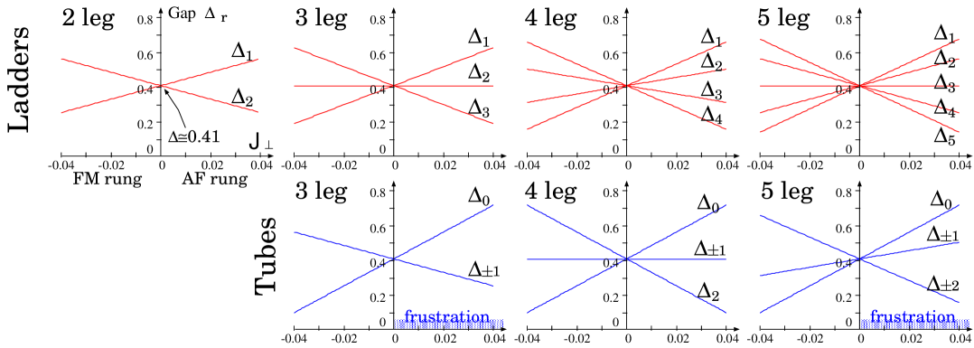
Figure 1: Gaps $\Delta_{r}$ versus rung coupling $J_{\perp}$ in the $N$-leg spin-1 AF systems (1) with $J=1$. The quantity $\Delta$ is the Haldane gap of the spin-1 AF chain $\hat{\cal H}_{0}$.

The new dispersion (24) and Fig. 1 elucidate several features of the magnon-band splitting.

(i) For ladder systems ($N^{\prime}=N-1$), the band splittings in both AF and ferromagnetic (FM) rung-coupling cases occur in the same way. Namely, the band structure depends on the magnitude of the rung coupling, $|J_{\perp}|$, but does not on the sign of $J_{\perp}$. This is because the term $J_{\perp}\sum_{n}\vec{m}_{n}\cdot\vec{m}_{n+1}$ changes its sign via the unitary transformation $\vec{m}_{n=\rm{even}}\to-\vec{m}_{n=\rm{even}}$, and the same transformation does not affect $\hat{\cal P}_{\rm{one}}$ and the effective theory for the unperturbed part, $N$ decoupled NLSMs. The difference between AF- and FM-rung sides would appear in higher-order corrections of the term $J_{\perp}\sum_{n}\vec{u}_{n}\cdot\vec{u}_{n+1}$, which is invariant under the above transformation.

(ii) For the tubes ($N^{\prime}=N$), in addition to the magnon triplet, the extra double degeneracy $\omega_{r}^{1\rm{st}}(p)=\omega_{-r}^{1\rm{st}}(p)$ is present except for $r=0$ and $r=\frac{N}{2}$ modes [note that $\cos k_{r}=\cos(-k_{r})$]. This degeneracy is attributed to the symmetry of the $\pi$ rotation with respect to the diameter of the cross section of tubes, i.e., the parity symmetry along the rung direction (see Fig. 3 in Ref. MS05, ). Therefore, it must remain even if higher-order corrections are taken into account.

(iii) Like the ladder case, in even-leg tubes, sign change $J_{\perp}\sum_{n}\vec{m}_{n}\cdot\vec{m}_{n+1}\to-J_{\perp}\sum_{n}\vec{m}_{n}\cdot\vec{m}_{n+1}$ is possible via $\vec{m}_{n=\rm{even}}\to-\vec{m}_{n=\rm{even}}$. Therefore, the band structure in an even-leg AF-rung tube and that in the corresponding FM-rung one are identical. On the other hand, the band structure in an odd-leg AF-rung tube differs from that in the corresponding FM-rung one. This is because any transformation connecting AF- and FM-rung systems are absent in odd-leg tubes.

(iv) In odd-leg tubes, the lowest excitation is the triply [sixfold] degenerate band $\omega_{0}^{1\rm{st}}(p)$ [$\omega_{\pm(N-1)/2}^{1\rm{st}}(p)$] for the FM-rung [AF-rung] case: this could refer to an even-odd character in the tube system (1). The rung-coupling-driven lowest-gap reduction in odd-leg AF-rung tubes is smaller than that in odd-leg FM-rung ones. The asymmetric splitting between AF- and FM-rung sides in odd-leg tubes, and the even-odd character is due to geometrical frustration along the rung direction in odd-leg AF-rung tubes.

(v) The lowest magnon band in FM-rung tubes ($N\geq 3$) $\omega_{0}^{1\rm{st}}(p)$ and that in even-leg AF-rung tubes $\omega_{N/2}^{1\rm{st}}(p)$ are independent of the leg number $N$. On the other hand (as expected), that in all the other systems falls down with increasing $N$.

(vi) Perturbation theory shows that the lowest excitation gaps in all the $N$-leg systems are a monotonically decreasing function of $|J_{\perp}|$. However, as in Fig. 2, from the consideration of the strong-rung-coupling regime, one sees that when $-J_{\perp}$ ($J_{\perp}$) is much larger than $J$, the lowest gap is close to the Haldane gap of the spin-$N\times S$ AF chain and does not vanish (the gap of the $N$ spin problem in one rung, which order is $J_{\perp}$). Predicting such a behavior would be beyond the scope of the present approach based on perturbation theory in the rung coupling.

(vii) As we already stated in Sec. II.2, it is expected that as $S$ is increased, $Z$ and $v$, respectively, become close to $g=2/S$ and $2SJa_{0}$. This result suggests the relation

$$\lambda_{r}(p) \stackrel{{\scriptstyle S\rm{:large}}}{{\to}} \frac{4S^{2}J}{\sqrt{\Delta^{2}+4S^{2}J^{2}p^{2}a_{0}^{2}}}J_{\perp}\cos k_{r}.$$ (28)

Thus, we can infer that the band-splitting width monotonically increases with the growth of $S$.

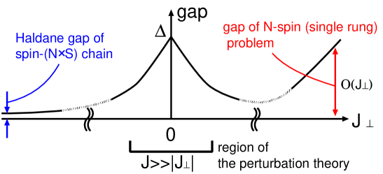
Figure 2: Expected lowest-gap profile in the $N$-leg integer-spin system (1). The symbol $\Delta$ means the Haldane gap of the spin-$S$ AF chain $\hat{\cal H}_{0}$. In the two-leg spin-1 case, the gap profile have already been predicted in Refs. Sene, , All, and Todo, .

The characteristic properties (i)-(vii) of the magnon-band structure in the weak-rung-coupling regime is completely consistent with our recent predictions based on the NLSM plus SPA analysis (see Sec. III A and Figs. 4-8 in Ref. MS05, ). The property (v) cannot explicitly be derived from NLSM plus SPA, but the right panel in Fig. 7 of Ref. MS05, implies it. We thus conclude that qualitative features of magnon bands predicted by our previous work in Ref. MS05, are supported by the present study. For more detailed physical interpretation of the results (i)-(vii), see Sec. III A of Ref. MS05, . The present study based on perturbation theory furthermore provides quantitative predictions on band structures in the weak-rung-coupling regime. In particular, the analytical expressions as in Eqs. (24)-(28) cannot be obtained in the previous NLSM plus SPA approach.

II.5 Quantitative comparison with quantum Monte Carlo Results

Here, we compare quantitatively the lowest-excitation gaps of $N$-leg systems evaluated by perturbation theory and those by QMC method. The QMC method cannot directly calculate the excitation gaps. However, it may be extracted from the proper correlation functions that can be calculated by the QMC.  T-K ; Todo ; Matsu0405

In Table 2, we summarize slopes of the lowest-excitation gaps of $N$-leg spin-1 AF systems (1) in the weak-rung-coupling limit, i.e., $-[d\Delta_{\rm min}/d|J_{\perp}|]_{J_{\perp}\to 0}$, where $\Delta_{\rm min}$ is the minimal gap in $\{\Delta_{r}\}$. Here, the slope data of QMC method (presented by Matsumoto) is defined by $(\Delta_{\rm min}|_{J_{\perp}=0}-\Delta_{\rm min}|_{|J_{\perp}|=0.01J})/(0.01J)$, where $\Delta_{\rm min}|_{J_{\perp}=0}$ is of course equal to the Haldane gap of the spin-1 AF Heisenberg chain $\hat{\cal H}_{0}$, $\Delta(S=1)=0.4105J$. In addition to Table 2, in Ref. Todo, , Todo and co-workers minutely investigate the slope of the gap of the two-leg spin-1 AF ladder in the extremely weak-rung-coupling regime, $|J_{\perp}|\leq 0.01J$, using QMC method (see Fig. 9 in Ref. Todo, ). They show that the slope is $\simeq 3.72$ in the AF-rung side, and is $\simeq 3.75$ in the FM-rung one. This is very close to the slope predicted by perturbation theory, $3.8$. From results of Ref. Todo, and the data in Table 2, we can conclude that perturbation theory is quantitatively valid in the sufficiently weak-rung-coupling regime, irrespective of leg number $N$.

Table 2: Slope of lowest gaps in $N$-leg spin-1 AF systems (1) near the decoupling point $J_{\perp}=0$, namely, $-[d\Delta_{\rm min}/d|J_{\perp}|]_{J_{\perp}\to 0}$. The data of QMC is evaluated by Munehisa Matsumoto.

		slope of lowest magnon gap
system	rung	QMC	perturbation theory
2-leg ladder	AF	$3.5$	$3.8$
	FM		$3.8$
3-leg ladder	AF	$5.0$	$5.4$
	FM		$5.4$
3-leg tube	AF		$3.8$
	FM		$7.65$
4-leg ladder	AF	$6.16$	$6.15$
	FM		$6.15$
4-leg tube	AF	$7.57$	$7.65$
	FM		$7.65$

In order to estimate the slope numerically, it is necessary to obtain the excitation gap in high precision for small rung couplings. In QMC method, the precise estimate of the gap is not easy because it has to be determined indirectly from correlation functions. On the other hand, our perturbation theory directly gives the slope, and thus is expected to be more reliable. Actually our prediction relies on the numerical estimates of $\Delta$, $v$, and $Z$. However, these are quantities defined on single chains, and can be determined accurately by numerical calculations. Moreover, we stress that QMC method does not work out well for frustrated (odd-leg, AF-rung) tubes because of so-called minus-sign problem. The present approach has an advantage that it can be applied even to those frustrated systems without any problem.

III ${\bm{N}}\to\infty$ limit and Higher Dimensions

The comparison with QMC results presented in Sec. II.5 implies that first-order perturbation results are efficient even for large $N$ (i.e., higher-order corrections are negligible at least in a sufficiently weak-rung-coupling case, even if $N$ is large). Assuming this is valid even in the $N\to\infty$ limit, we can present a few predictions for spatially anisotropic $d$-D ($d\geq 2$) spin systems, from the results in Sec. II.

In the $N\to\infty$ limit, the distribution of $k_{r}$ is dense. Therefore, the lowest-excitation modes $\omega_{r}^{1\rm{st}}(p)$ in all the infinite-leg (i.e., 2D) systems take $\cos k_{r}\to-1$ or $+1$. Particularly, for the FM-rung tube [even-leg AF-rung tube] cases, as we already mentioned in Sec. II.3, the lowest mode $\omega_{0}^{1\rm{st}}(p)$ [$\omega_{N/2}^{1\rm{st}}(p)$] always takes $\cos k_{0}=1$ [$\cos k_{N/2}=-1$] regardless of $N(\geq 3)$: namely, the lowest mode in the 2D system already exists in a corresponding 1D one with arbitrary $N$. From these properties in the $N\to\infty$ case, one finds that the slope of the gap reduction $-[d\Delta_{\rm min}/d|J_{\perp}|]_{J_{\perp}\to 0}$ is a finite value $2\omega_{\perp}(0)/J_{\perp}$ in the infinite-leg system (1). It means that [$A$] the Haldane phase (1D gapped spin liquid) still survives in the 2D spatially anisotropic integer-spin AF system if the exchange coupling in the chain direction is extremely strong, and [$B$] there is a finite critical value of $J_{\perp}$ ($J_{\perp}^{c}$) which lies between the Haldane phase and the Néel ordered one. This prediction is consistent with results of previous studies. S-T ; Matsu ; Tasaki ; Sene2 ; K-K

For the 2D spin-1 spatially anisotropic AF Heisenberg model [i.e., an infinite-leg spin-1 AF system (1) with $J_{\perp}>0$], the critical value $J_{\perp}^{c}$ has been numerically evaluated: for instance, the chain-mean-field plus exact-diagonalization analysis, S-T the cluster-expansion method, K-K and the QMC simulation Matsu conclude $J_{\perp}^{c}\gtrsim 0.025J$, $\simeq 0.056J$, and $\simeq 0.04365J$, respectively. On the other hand, perturbation theory provides the slope of the gap $2\omega_{\perp}(0)/J_{\perp}\simeq 7.65$ for the spin-1, $N\to\infty$ case. As we explain in Fig. 3, a naive extrapolation of the linear behavior gives a vanishing of the gap at a finite $J_{\perp}$. This may be identified with the critical value, within the present framework. It leads to $|J_{\perp}^{c}|\simeq 0.05J$. This is again consistent with the above numerical estimates. We emphasize that the critical values $J_{\perp}^{c}$ for both AF- and FM-rung cases have the same magnitude in the first-order perturbation theory. This prediction also agrees with a recent QMC result. Matsu_pre

These results and those in Sec. II indicate that perturbation theory is quantitatively reliable for any $N$-leg integer-spin AF system, including the $N\to\infty$ case.

As one readily expects, the above discussion of the 2D system can be generalized to $d$-D lattice cases. Namely, following the similar calculation of the first-order perturbation in Sec. II.3, we can show that for a $N^{d-1}$-leg system on a $d$-D lattice, the lowest-magnon-gap slope also remains finite at the $N\to\infty$ limit, like the case of ladders or tubes. For instance, the lowest gap of a weakly coupled integer-spin AF chains on $d$-D hypercubic lattice is evaluated as

$$\Delta_{d} = \Delta-\frac{S^{2}Zv}{\Delta a_{0}}\sum_{a=2}^{d}|J_{\perp}^{(a)}|,$$ (29)

where $J_{\perp}^{(a)}$ is the interchain exchange in $a$th direction (the first direction is that of the chain). Moreover, in the case of $J_{\perp}^{(a)}=J_{\perp}$, the slope of the gap is determined as $-d\Delta_{d}/d|J_{\perp}|=\frac{(d-1)S^{2}Zv}{\Delta a_{0}}$: in the spin-1, 3D case, the slope is $\simeq 15.3$, twice $2\omega_{\perp}(0)/J_{\perp}$. Thus, our first-order perturbation theory suggests that a gapped phase exists if all the interchain couplings are weak enough in any $d$-D spatially anisotropic integer-spin AF system. This prediction is consistent with the general belief that gapped phases are robust against small perturbations.

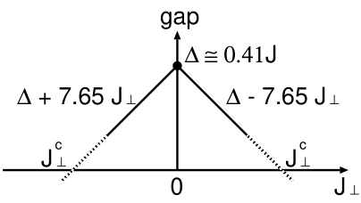
Figure 3: Lowest excitation gap and critical point $J_{\perp}^{c}$ for the $N\to\infty$, spin-1 case predicted by perturbation theory. The quantity $\Delta$ is the Haldane gap of the spin-1 AF chain $\hat{\cal H}_{0}$.

IV Rung-coupling decorations

As we already mentioned, perturbation theory, in principle, can deal with any sorts of interchain interactions. Therefore, in this section, as a generalization of the standard coupling $\hat{\cal H}_{\perp}$, let us briefly investigate the following typical frustrated rung coupling:

$$\hat{\cal H}^{\prime} = \hat{\cal H}_{\perp}+\hat{\cal H}_{1}+\hat{\cal H}_{2},$$

$$\hat{\cal H}_{1} = K_{1}\sum_{n,j}\vec{S}_{n,j}\cdot\vec{S}_{n+1,j+1},$$

$$\hat{\cal H}_{2} = K_{2}\sum_{n,j}\vec{S}_{n,j}\cdot\vec{S}_{n+1,j-1}.$$ (30)

This coupling is illustrated in Fig. 4. For example, an infinite-leg system with $K_{1}\neq 0$ and $K_{2}=0$ ($K_{1}=K_{2}$) may be called a spatially anisotropic model on triangular lattice (spatially anisotropic $J_{1}$-$J_{2}$-like model). It is noteworthy that in contrast to the standard case of $\hat{\cal H}^{\prime}=\hat{\cal H}_{\perp}$, when $\hat{\cal H}_{1({\rm or}\,2)}$ is present alone, odd-leg FM-rung tubes exhibits geometrical frustration.

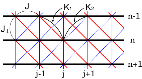
Figure 4: Decorated rung couplings.

As in the case of $\hat{\cal H}^{\prime}=\hat{\cal H}_{\perp}$, the first-order correction of the ground-state energy, $\langle\Phi|\hat{\cal H}_{1,2}|\Phi\rangle$, are zero. Furthermore, the effective Hamiltonians for $\hat{\cal H}_{1,2}$ in the one-magnon space are easily obtained in the similar way from Eq. (12) to Eq. (13). The results are

$$\hat{\cal H}_{1,2}^{1\rm{st}} \equiv \hat{\cal P}_{\rm{one}}\hat{\cal H}_{1,2}\hat{\cal P}_{\rm{one}}=\sum_{\alpha}\sum_{n=1}^{N^{\prime}}\int\frac{vdp}{4\pi\omega(p)}\left(-\frac{S^{2}Zv}{2\omega(p)a_{0}}K_{1,2}\right)\Big{[}|p,\alpha,n\rangle e^{\pm ipa_{0}}\langle p,\alpha,n+1|+{\rm H.c.}\Big{]}.$$ (31)

The exponential factors $\exp(\pm ipa_{0})$ come from the fields $\vec{m}_{n}(x\pm a_{0})$ in $\hat{\cal H}_{1,2}$. In ladder cases, if the rung coupling $\hat{\cal H}^{\prime}$ contains only $\hat{\cal H}_{1}$ or $\hat{\cal H}_{2}$, the factors could be replaced with unity by taking the field redefinition $\vec{m}_{n}(x\pm a_{0})\to\vec{\tilde{m}}_{n}(x)$ at the intermediate stage in the derivation of Eq. (31). The replacement is physically reasonable, because a ladder system with $\hat{\cal H}^{\prime}=\hat{\cal H}_{\perp}$ is equivalent to one with $\hat{\cal H}^{\prime}=\hat{\cal H}_{1\,({\rm or}\,2)}$ and $K_{1\,({\rm or}\,2)}=J_{\perp}$. However, one has to note that such a replacement procedure is not allowed when more than two kinds of rung couplings are simultaneously present. Using Eq. (31) and results of eigenvalue problems in Appendix A, we obtain the following magnon bands of $N$-leg systems with a generalized rung coupling $\hat{\cal H}^{\prime}$:

$$\tilde{\omega}_{r}^{1\rm st}(p) = \sqrt{\Delta^{2}+p^{2}v^{2}}+\frac{S^{2}Zva_{0}^{-1}}{\sqrt{\Delta^{2}+p^{2}v^{2}}}\times\left\{\begin{array}[]{ccc}|J_{\perp}-K_{1}e^{-ipa_{0}}-K_{2}e^{ipa_{0}}|\cos(k_{r}+\theta)&{\rm tubes},\\ |J_{\perp}-K_{1}e^{-ipa_{0}}-K_{2}e^{ipa_{0}}|\cos k_{r}&{\rm ladders},\\ \end{array}\right.$$ (34)

where the angle $\theta$ is defined by $J_{\perp}-K_{1}e^{-ipa_{0}}-K_{2}e^{ipa_{0}}=|J_{\perp}-K_{1}e^{-ipa_{0}}-K_{2}e^{ipa_{0}}|e^{i\theta}$. In the dispersion relation, the phase of $e^{\pm ipa_{0}}$ may be negligible around $p=0$. While, when $p$ becomes too large (order of $\pi/a_{0}$), and thus the deviation between $e^{\pm ipa_{0}}$ and unity becomes clear, the present NLSM picture for the $N$-leg system is less reliable.

In the case of $J_{\perp}=K_{1}+K_{2}$, the magnon-band degeneracy around $p=0$ is not lifted by the first-order correction of the rung coupling $\hat{\cal H}^{\prime}$. This must be due to frustration among $\hat{\cal H}_{\perp}$, $\hat{\cal H}_{1}$, and $\hat{\cal H}_{2}$. From this prediction, we can expect that the gapped-phase region in the infinite-leg system with a frustrated rung coupling are much larger than that in the standard system with $\hat{\cal H}^{\prime}=\hat{\cal H}_{\perp}$ (see Sec. III). This is consistent with a recent work using DMRG. Mou

V Summary

In this paper, utilizing only the information about integer-spin AF chains $\hat{\cal H}_{0}$ (exact results of the NLSM, and values of $\Delta$, $v$, and $Z$), we have formulated a first-order perturbation expansion in the rung-coupling strength for the $N$-leg integer-spin system (1). All the magnon excitation energies have been quantitatively predicted as in Eqs. (24)-(26) and Fig. 1. Several features of the magnon excitation structure have been elucidated [see comments (i)-(vii) in Sec. II.4]. The results of perturbation theory are supported by the QMC data and agree with our recent study based on NLSM and SPA in Ref. MS05, . We further applied the perturbation method to cases of $N\to\infty$ and systems with a generalized rung coupling in Secs. III and IV, respectively. Particularly, in Sec. III, it is predicted that a Haldane state (gapped state with 1D nature) survives in spatially anisotropic $d$-D ($d\geq 2$) integer-spin AF systems, if the exchange coupling of one direction are sufficiently larger than all others [see Eq. (29)]. This agrees with several previous studies based on different methods. S-T ; Matsu ; Tasaki ; Sene2 ; K-K We expect that if fitting parameters $\Delta$, $v$, and $Z$ are more accurately calculated, perturbation theory leads to almost exact predictions in the weak-rung-coupling regime.

The perturbation theory approach has some advantages over other methods. (i) It can lead to not only the lowest magnon band, but also all other magnon ones. (ii) One can predict several quantities with analytical expressions if nonuniversal parameters $(\Delta,v,Z)$ are given. (iii) Perturbation theory is expected to be applicable to all the systems with any leg number $N$. Therefore, as one found in Secs. II and III, the dimensional crossover behavior (how a 1D $N$-leg system approaches the corresponding $d$-D one when $N$ becomes large) can be partially described. (iv) It is possible to investigate any kind of interchain interactions.

We have thus demonstrated that the very simple perturbation theory can give nontrivial results on weakly coupled integer-spin AF chains. Within the first order, perturbation theory is reduced to an eigenvalue problem in finite dimensions thanks to various selection rules [see Eq. (8)]. The precise numerical data known for the single chain then enables us to make quantitative predictions in the weak-rung-coupling regime.

Similar approach should also be useful for more general quasi-1D systems consisting of weakly coupled gapped 1D systems. When the 1D system is gapless, perturbation theory is not quite easy. Usually, we have to rely on renormalization-group arguments, as in the case of the well-studied two-leg ladder consisting of spin-$\frac{1}{2}$ AF chains.

Appendix A Tridiagonal Matrices

Here, we briefly summarize solutions of eigenvalue problems of the following $N\times N$ Hermitian matrices,

$${\cal A} = \left(\begin{array}[]{cccccccc}A_{1}&A_{2}&&&A_{2}^{*}\\ A_{2}^{*}&A_{1}&\ddots&&\\ &\ddots&\ddots&\ddots&\\ &&\ddots&\ddots&A_{2}\\ A_{2}&&&A_{2}^{*}&A_{1}\\ \end{array}\right),$$ (35f)

$${\cal B} = \left(\begin{array}[]{cccccccc}B_{1}&B_{2}&&&\\ B_{2}^{*}&B_{1}&\ddots&&\\ &\ddots&\ddots&\ddots&\\ &&\ddots&\ddots&B_{2}\\ &&&B_{2}^{*}&B_{1}\\ \end{array}\right).$$ (35l)

The case in which $A_{2}$ and $B_{2}$ contain an imaginary part is not discussed well in literature.

The eigenvalue problem for the matrix $\cal A$ ($N\geq 3$) is easily solved by the Fourier transformation method. The eigenvalues $\alpha_{r}$ and the corresponding eigenvectors $\vec{A}_{r}$ are given by

$$\alpha_{r} = A_{1}+2|A_{2}|\cos(k_{r}+\theta),\,\,\,\,\,\,k_{r}=\frac{2r}{N}\pi,$$ (36a)

$$\vec{A}_{r} = \sqrt{\frac{2}{N}}\,\,{}^{T}\Big{(}e^{ik_{r}},e^{2ik_{r}},\dots,e^{Nik_{r}}\Big{)},$$ (36b)

where the angle $\theta$ is defined by $A_{2}=|A_{2}|e^{i\theta}$, $r=0,\dots,N-1$ (mod $N$), and $\vec{A}_{r}^{2}=1$. On the other hand, the matrix ${\cal B}$ can be diagonalized by assuming that the $n$th component of each eigenvector satisfies $b_{n}\propto e^{-in\phi}\sin(kn)$ where the angle $\phi$ is the argument of $B_{2}$ ($B_{2}=|B_{2}|e^{i\phi}$) and $k$ is a constant. As a result, the eigenvalues $\beta_{r}$ and the eigenvectors $\vec{B}_{r}$ are

$$\beta_{r} = B_{1}+2|B_{2}|\cos k_{r},\,\,\,\,\,\,k_{r}=\frac{r}{N+1}\pi,$$ (37a)

$$\vec{B}_{r} = \sqrt{\frac{2}{N+1}}{}^{T}\Big{(}e^{-i\phi}\sin k_{r},e^{-i2\phi}\sin 2k_{r},$$ (37b)

$$\hskip 56.9055pt\dots,e^{-iN\phi}\sin Nk_{r}\Big{)},$$

where $r=1,\dots,N$ and $\vec{B}_{r}^{2}=1$.

Appendix B Spin correlation functions in integer-spin AF chains

We demonstrate how the NLSM scheme derives the asymptotic form of spin correlation functions in the integer-spin AF chain $\hat{\cal H}_{0}$. As shown below, comparing the resulting form and that estimated by a numerical method, the factor $Z$, etc. can be determined.

As we said in the main text, the low-energy physics of the chain $\hat{\cal H}_{0}$ is described by the NLSM (2). From the formula (3), the long-distance behavior of the equal-time two-point spin correlation is represented as

$$\lim_{|j-k|\to\infty}\langle S_{j}^{\alpha}S_{k}^{\alpha}\rangle \approx (-1)^{|j-k|}S^{2}\langle m^{\alpha}(x_{j})m^{\alpha}(x_{k})\rangle$$ (38)

$$+\langle u^{\alpha}(x_{j})u^{\alpha}(x_{k})\rangle,$$

where $x_{j(k)}=j(k)\times a_{0}$. The term $\langle u^{\alpha}m^{\alpha}\rangle$ disappears due to the symmetry of $\vec{m}\to-\vec{m}$. Because $\vec{m}$ and $\vec{u}$ are one-magnon and two-magnon fields respectively, the most relevant part at $|j-k|\to\infty$ is the first staggered term. Using the projection operators in Eq. (7), we estimate it as follows:

$$\langle m^{\alpha}(x)m^{\alpha}(0)\rangle = \Big{\langle}m^{\alpha}(x)\Big{[}\sum_{s}\hat{\cal P}_{s}\Big{]}m^{\alpha}(0)\Big{\rangle}$$ (39)

$$= \langle m^{\alpha}(x)\hat{\cal P}_{1}m^{\alpha}(0)\rangle+\dots$$

$$= \frac{Zv}{4\pi}\int dp\frac{e^{ipx}}{\sqrt{\Delta^{2}+p^{2}v^{2}}}+\dots$$

$$= \frac{Z}{2\pi}K_{0}(|x|/\xi)+\dots$$

$$\stackrel{{\scriptstyle x\to\infty}}{{\approx}} \frac{Z}{\sqrt{8\pi|x|/\xi}}\,\,e^{-|x|/\xi},$$

where $\xi=v/\Delta$ is the correlation length and $K_{0}(x)$ is the modified Bessel function. If correct values of the spin-wave velocity $v$ and the Haldane gap $\Delta$ are already known, the comparison between the spin correlation determined by Eqs. (38) and (39), and the one done by a numerical method can fix the parameter $Z$. Actually, the value of $Z$ in Table 1 is determined by such a method. A-W ; S-A

In the similar way from Eq. (38) to Eq. (39), the long-(imaginary)time behavior of the equal-position two-point spin correlation function is evaluated as

$$\langle S_{j}^{\alpha}(\tau)S_{j}^{\alpha}(0)\rangle \approx S^{2}\langle m^{\alpha}(x,\tau)m^{\alpha}(x,0)\rangle$$ (40)

$$\approx \frac{S^{2}Zv}{4\pi}\int dp\frac{e^{-\omega(p)\tau}}{\omega(p)}$$

$$= i\frac{S^{2}Z}{4}H_{0}^{(1)}(i\Delta\tau)$$

$$\stackrel{{\scriptstyle\tau\to\infty}}{{\approx}} \frac{S^{2}Z}{\sqrt{8\pi\Delta\tau}}\,\,e^{-\Delta\tau},$$

where $\tau(=it)>0$ is the imaginary time, $S_{j}^{\alpha}(\tau)=e^{\hat{\cal H}_{0}\tau}S_{j}^{\alpha}e^{-\hat{\cal H}_{0}\tau}$, $m^{\alpha}(x,\tau)=e^{\hat{\cal H}_{0}\tau}m^{\alpha}(x)e^{-\hat{\cal H}_{0}\tau}$, and $H_{0}^{(1)}(x)$ is the Hankel function of the first kind. The form (40) is an expected result from Eq. (39) (because the NLSM is a relativistic system).

Appendix C Higher-order Terms

We briefly consider higher than second-order corrections in the $N$-leg system (1). In principle, following the standard manner of perturbation theory, one would perform calculations up to any order. However, as one will see below, there is a difficulty in extracting quantitative predictions from higher-order terms within the perturbation theory framework of the main text.

Generally, a second-order perturbation term is represented as

$$\int\prod_{q=1}^{Q}\frac{vdp_{q}}{4\pi\omega(p_{q})}\langle A|\hat{\cal H}_{\perp}|Q\rangle\frac{1}{E_{A}-E_{Q}}\langle Q|\hat{\cal H}_{\perp}|A\rangle,$$ (41)

where $|A\rangle$ is an eigenstate of the unperturbed system $\hat{\cal H}_{\parallel}$ with an energy $E_{A}$ and a momentum $P_{A}$, and similarly $|Q\rangle$ stands for a $Q$-magnon state with an energy $E_{Q}=\sum_{q}\omega(p_{q})$ and a momentum $P_{Q}=\sum_{q}p_{q}$ ($p_{q}$ is the momentum of each magnon). The matrix element $\langle A|\hat{\cal H}_{\perp}|Q\rangle$ in the integrand would contain

$$I(A,Q)J_{\perp}\int\frac{dx}{a_{0}}e^{i(P_{Q}-P_{A})x},$$ (42)

where the factor $I(A,Q)$ is independent of $x$. Therefore, noticing that $\int dxe^{i(P_{Q}-P_{A})x}=2\pi\delta(P_{Q}-P_{A})$ and $\delta(P_{Q}-P_{A})^{2}\sim L\times\delta(P_{Q}-P_{A})$ where $L$ is the chain length, we expect that a second-order term generally generates a quantity of $O(L)$. Actually, one can easily verify that in the second-order ground-state energy correction, the term originating from the lowest-energy intermediate states with two magnons is $O(L)$. Under the assumption that one-magnon states still take the lowest excitation when a finite rung coupling is added in decoupled chains $\hat{\cal H}_{\parallel}$, all $O(L)$ second-order perturbation terms for the ground state must completely cancel out those for one-magnon states at least in the thermodynamic limit ($L\to\infty$). Only $O(L^{0})$ terms, if they are present, can contribute to the second-order correction of the magnon-band splitting in the limit.

These arguments appear to suggest that almost all the second-order perturbation terms are $O(L)$. However, the factor $I(A,Q)$ in Eq. (42) can possess a finite-size correction; for instance, the parameter $Z=|\langle 0|m^{\alpha}(0)|p,\alpha\rangle|^{2}$ might be expanded as $Z=Z(L)=Z_{0}+Z_{1}/L+Z_{2}/L^{2}+\dots$ ($Z$ in Table 1 stands for $Z_{0}$). Furthermore, $v$ and $\Delta$ must also have a finite-size effect. Such finite-size corrections could generate an $O(L^{0})$ term. Unfortunately, as far as we know, finite-size correction terms have never been quantitatively estimated. Therefore, we cannot derive quantitative predictions from the second-order perturbation expansion.

The similar difficulty also emerges in calculations of higher than third-order corrections. Thus, we can conclude that it is generally hard to quantitatively calculate higher-order terms in the scheme in this paper. Using the above expansion $Z(L)=Z_{0}+Z_{1}/L+\dots$, one might obtain some qualitative features of higher-order corrections in the magnon-band splitting.

References

- (1) H. J. Schulz, cond-mat/9605075.
- (2) G. Sierra, J. Phys. A 29, 3299 (1996): see also cond-mat/9610057.
- (3) A. O. Gogolin, A. A. Nersesyan and A. M. Tsvelik, Bosonization and Strongly Correlated Systems (Cambridge University Press, Cambridge, England, 1998).
- (4) T. Giamarchi, Quantum Physics in One Dimension (Oxford University Press, New York, 2004).
- (5) A. Gozar and G. Blumberg, in Frontiers in Magnetic Materials, edited by A.V. Narlikar, p.653 (Springer-Verlag 2005); see also cond-mat/0510193.
- (6) M. Azuma, Z. Hiroi, M. Takano, K. Ishida, and Y. Kitaoka, Phys. Rev. Lett. 73, 3463 (1994).
- (7) K. Kojima, A. Keren, G. M. Luke, B. Nachumi, W. D. Wu, Y. J. Uemura, M. Azuma, and M. Takano, Phys. Rev. Lett. 74, 2812 (1995).
- (8) K. Kawano and M. Takahashi, J. Phys. Soc. Jpn. 66, 4001 (1997).
- (9) J. Schnack, H. Nojiri, P. Kögerler, G. J. T. Cooper and L. Cronin, Phys. Rev. B 70, 174420 (2004).
- (10) P. Millet, J. Y. Henry, F. Mila and J. Galy, J. Solid State Chem. 147, 676 (1999).
- (11) A. Lüscher, R. M. Noack, G. Misguich, V. N. Kotov and F. Mila, Phys. Rev. B 70, 060405(R) (2004).
- (12) J.-B. Fouet, A. Läuchli, S. Pilgram, R. M. Noack and F. Mila, Phys. Rev. B 73, 014409 (2006).
- (13) K. Okunishi, S. Yoshikawa, T. Sakai, and S. Miyashita, Prog. Theor. Phys. Supp. 159, 297 (2005).
- (14) A. G. Rojo, Phys. Rev. B 53, 9172 (1996).
- (15) M. Oshikawa, M. Yamanaka and I. Affleck, Phys. Rev. Lett. 78, 1984 (1997).
- (16) S. Dell’Aringa, E. Ercolessi, G. Morandi, P. Pieri, and M. Roncaglia, Phys. Rev. Lett. 78, 2457 (1997).
- (17) M. Matsumoto, C. Yasuda, S. Todo, and H. Takayama, Phys. Rev. B 65, 014407 (2001).
- (18) C. Yasuda, S. Todo, K. Hukushima, F. Alet, M. Keller, M. Troyer, and H. Takayama, Phys. Rev. Lett. 94, 217201 (2005).
- (19) M. Sato, Phys. Rev. B 72, 104438 (2005).
- (20) D. Sénéchal, Phys. Rev. B 52, 15319 (1995).
- (21) M. Matsumoto et al, The Physical Society of Japan Autumn Meeting (2003); The Physical Society of Japan 59th Annual Meeting (2004).
- (22) M. Matsumoto et al, in preparation.
- (23) F. D. M. Haldane, Phys. Rev. Lett. 50, 1153 (1983).
- (24) E. Fradkin, Field Theories of Condensed Matter Systems (Addison-wesley, 1991).
- (25) A. Auerbach, Interacting Electrons and Quantum Magnetism (Springer-Verlag, New York, 1994).
- (26) M. D. P. Horton and I. Affleck, Phys. Rev. B 60, 11891 (1999).
- (27) F. H. L. Essler, Phys. Rev. B 62, 3264 (2000).
- (28) I. Affleck and R. A. Weston, Phys. Rev. B 45, 4667 (1992).
- (29) E. S. Sørensen and I. Affleck, Phys. Rev. B 49, 13235 (1994); 49, 15771 (1994).
- (30) S. Qin, X. Wang, and L. Yu, Phys. Rev. B 56, R14251 (1997).
- (31) S. Todo and K. Kato, Phys. Rev. Lett. 87, 047203 (2001).
- (32) D. Allen and D. Sénéchal, Phys. Rev. B 61, 12134 (2000).
- (33) S. Todo, M. Matsumoto, C. Yasuda and H. Takayama, Phys. Rev. B 64, 224412 (2001).
- (34) T. Sakai and M. Takahashi, Phys. Rev. B 42, 4537 (1990).
- (35) H. Tasaki, Phys. Rev. Lett. 64, 2066 (1990).
- (36) D. Sénéchal, Phys. Rev. B 48, 15880 (1993).
- (37) A. Koga and N. Kawakami, Phys. Rev. B 61, 6133 (2000).
- (38) S. Moukouri, J. Stat. Mech.: Theory Exp. 2006, P02002.