Thermal collapse of a granular gas under gravity

Abstract

Free cooling of a gas of inelastically colliding hard spheres represents a central paradigm of kinetic theory of granular gases. At zero gravity the temperature of a freely cooling homogeneous granular gas follows a power law in time. How does gravity, which brings inhomogeneity, affect the cooling? We combine molecular dynamics simulations, a numerical solution of hydrodynamic equations and an analytic theory to show that a granular gas cooling under gravity undergoes thermal collapse: it cools down to zero temperature and condenses on the bottom of the container in a finite time.

Granular gas, a low-density fluid of inelastic hard spheres, is a simple model of granular flow, and it has attracted much attention from physicists Haff ; Goldhirsch+BP . An undriven granular gas loses its kinetic energy via inelastic collisions. In the Homogeneous Cooling State (HCS) the temperature $T$ of a dilute granular gas decays according to Haff’s law Haff , $T(t)=T_{0}(1+t/t_{0})^{-2}$, where in two dimensions $t_{0}=\sqrt{\pi/2}\,(1-r^{2})\,dn_{0}T_{0}^{1/2}$ is the cooling time, $n_{0}$ is the (constant) number density of the particles, $d$ is the particle diameter and $r$ is the coefficient of normal restitution. The HCS, and deviations from it, provide a rich testing ground for the ideas and methods of kinetic theory of granular gases, and it has been investigated in many theoretical works, see Ref. Goldhirsch+BP and references therein. Direct experimental observation on the HCS is difficult, not the least because of gravity. Therefore it is somewhat surprising that there have been no theoretical studies of the effect of gravity on the free cooling of a granular gas. It is intuitively clear that gravity forces grains to sink to the bottom of the container, where increased density enhances the collision rate and causes “freezing” of the granulate. However, no quantitative analysis of this process has ever been performed. Here we combine molecular dynamics (MD) simulations, a numerical solution of granular hydrodynamic equations and analytical theory to develop a detailed quantitative understanding of this cooling process. Our main result is that, in a striking contrast to Haff’s law, the gas undergoes thermal collapse: it cools down to zero temperature and condenses on the bottom plate in a finite time exhibiting, close to collapse, a previously unknown universal scaling behavior.
MD simulations. We employed an event-driven algorithm Rapaport to simulate a free cooling of an initially dilute gas of $N\gg 1$ identical nearly elastic, $1-r\ll 1$, hard disks of unit diameter and mass in a two-dimensional container of width $L_{x}$ and infinite height. The (elastic) bottom of the container is at $y=0$, the (elastic) side walls are at $x=0$ and $L_{x}$. $L_{x}$ is chosen small enough so that any macroscopic structure in the lateral direction is suppressed. The gravity acceleration $g$ acts in the negative $y$ direction. Figure 1 shows four snapshots of a typical simulation where, at $t=0$, particles have a Maxwell velocity distribution, and a Boltzmann density profile at constant temperature $T_{0}$ isothermal . Collapse of all particles to the bottom is observed at time $t_{c}=7770$. The circles in Fig. 2a show the time history of the simulated total kinetic energy of the gas, normalized to its value at $t=0$. One can see that the total energy drops to zero in a finite time. We observed a similar behavior in a wide range of parameters, and also for a different, non-isothermal initial state, prepared by replacing the elastic bottom plate by a “thermal” bottom plate Rapaport and waiting until a steady state is reached. In the latter case the initial transient is somewhat different, but the energy decay law close to collapse remains the same, see Fig. 2a.

Figure 1: Snapshots of an event-driven MD simulation at indicated times for $N=5642$, $L_{x}=10^{2}$, $r=0.995$, $T_{0}=10$ and $g=0.01$. Only a part of the box is shown.

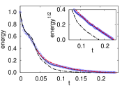
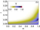
Figure 2: (a) Total kinetic energy of the grains, normalized to its value at $t=0$, vs. time for the run in Fig. 1 (circles). Also shown are the results from the full hydrodynamic model (1)-(3) (black solid line), from the $\omega$-equation (4) (red dashed line), and from a MD simulation with a different, non-isothermal initial condition (black dash-dotted line). The respective hydrodynamic parameters are $\varepsilon=10^{-2}$ and $\Lambda=5$. The inset shows the square root of the energy close to thermal collapse. (b) a space-time plot of $T$ from the full hydrodynamic model for the same simulation.

Hydrodynamic theory. The observed energy decay dynamics are remarkably captured by hydrodynamic equations for the number density $n(y,t)$, vertical velocity $v(y,t)$ and granular temperature $T(y,t)$. These equations are systematically derivable from the Boltzmann equation generalized to account for inelastic collisions of hard disks Goldhirsch+BP . We assume a dilute gas, an assumption which becomes invalid close to collapse. Following Ref. bromberg03 , we rescale the variables using the gravity length scale $\lambda=T_{0}/g$ and the heat diffusion time $t_{d}=\varepsilon^{-1}(\lambda/g)^{1/2}$. The scaled parameter $\varepsilon=\pi^{-1/2}(L_{x}/Nd)\ll 1$ is of the order of the inverse number of layers of grains which form after the particles settle on the bottom. The smallness of $\varepsilon$ guarantees that $t_{d}$ is much longer than the fast hydrodynamic time $t_{f}=(\lambda/g)^{1/2}$. We measure $v$ in units of $v_{0}=\lambda/t_{d}$, $n$ in units of $n_{0}=N/\lambda L_{x}$, and $T$ in units of $T_{0}$. Furthermore, we exploit the one-dimensionality of the flow and go over to Lagrangian mass coordinate $m=\int_{0}^{y}n(y^{\prime},t)dy^{\prime}$ which varies between $0$ at the bottom and $1$ (the total rescaled mass of the gas) as $y\to\infty$. The resulting rescaled hydrodynamic equations are bromberg03 ; Fourier :

$$\partial_{t}(1/n)=\partial_{m}v\,,$$ (1)

$$\varepsilon^{2}\partial_{t}v=-\partial_{m}(nT)-1+(\varepsilon^{2}/2)\,\partial_{m}(nT^{1/2}\partial_{m}v)\,,$$ (2)

$$\partial_{t}T+nT\partial_{m}v=(\varepsilon^{2}/2)\,nT^{1/2}(\partial_{m}v)^{2}+$$

$$(4/3)\,\partial_{m}(n\partial_{m}T^{3/2})-4\Lambda^{2}nT^{3/2}\,,$$ (3)

In addition to $\varepsilon$, Eqs. (1)-(3) include the parameter $\Lambda^{2}=\frac{1-r^{2}}{4\varepsilon^{2}}$ which shows the relative role of the inelastic energy loss and heat diffusion. At the boundaries $y=0$ and $\infty$ we demand zero fluxes of mass, momentum and energy bromberg03 , which yield $v=\partial_{m}T=0$ at $m=0$ and $n\partial_{m}v=n\partial_{m}T=0$ at $m=1$.

We solved Eqs. (1)-(3) numerically in a wide range of parameters, using a variable mesh/variable time step solver solver . The blue solid line in Fig. 2a depicts the sum of the thermal energy and macroscopic kinetic energy of the gas versus time for the same parameters and initial condition as in the MD simulation indicated by the circles. The agreement is excellent, and thermal collapse is clearly observed condensate . At the very early stage of the cooling [with duration of ${\mathcal{O}}(\tau_{f})$] we observed shock waves which form at large heights, cause a transient heating of the gas there, and escape to $m=1$ ($y=\infty$), see Fig. 2b.

Quasi-static flow. If $\varepsilon\ll\min(1,\Lambda^{-2})$ then, after the brief transient, a quasi-static flow sets in. Here the $\varepsilon^{2}$-terms in Eqs. (2) and (3) can be neglected, and Eq. (2) reduces to the hydrostatic condition $\partial_{m}(nT)+1=0$ which yields $nT=1-m$. Substituting $n=(1-m)/T$ into Eq. (3) and using Eq. (1), we obtain a closed nonlinear equation for a new variable $\omega(m,t)=T^{1/2}(m,t)$:

$$\omega\partial_{t}\omega=\partial_{m}\left[(1-m)\partial_{m}\,\omega\right]-\Lambda^{2}(1-m)\omega\,,$$ (4)

We will call Eq. (4) the $\omega$-equation; it was derived, in another context, in Ref. bromberg03 .

We solved the $\omega$-equation numerically [with the no-flux boundary conditions $(1-m)\partial_{m}\omega=0$ at $m=0$ and $1$], using the same solver solver . A typical example is shown in Fig. 2a. Here we launched the computation at scaled time $t=0.04$ when the hydrostatic condition $nT=1-m$ already holds well, and used the temperature profile, computed with the full hydrodynamic solver, as the initial condition. One can see that the $\omega$-equation provides a faithful description of the later stage of the cooling. Figure 3 shows a different example of the cooling dynamics, as described by the $\omega$-equation starting from $\omega(m,t=0)=1$. Here we show the $T$- and $v$-profiles in both Lagrangian and Eulerian coordinates. In all simulations thermal collapse is observed at a time $t_{c}$ which goes down as $\Lambda$ increases. The collapse occurs simultaneously on the whole Lagrangian interval $(0,1)$, see Fig. 3a. As the density $n=(1-m)/T$ blows up at $t=t_{c}$ at all $m\in[0,1)$, this Lagrangian interval corresponds to a single Eulerian point $y=0$. Therefore, at time $t=t_{c}$ all of the gas condenses on the bottom plate $y=0$ and cools to a zero temperature different .

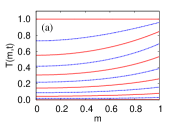
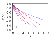
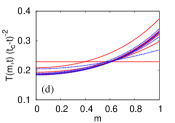
Figure 3: Hydrodynamic fields predicted by the $\omega$-equation for $\Lambda=1$: $T(m,t)$ at times separated by $\Delta t=0.2$ (a), and $T(y,t)$ (b), $v(y,t)$ (c), and $T(m,t)(t_{c}-t)^{-2}$ (d) at the same times. The late-time curves in d collapse into a single curve.

Separable solution close to collapse. As Fig. 3d implies, $\omega(m,t)$ becomes separable as $t\to t_{c}$. This remarkable solution can be written as

$$\omega(m,t)=(t_{c}-t)\,Q(m)\,,$$ (5)

where $Q(m)$ is determined by the nonlinear ODE

$$\left[(1-m)Q^{\prime}\right]^{\prime}-\Lambda^{2}(1-m)Q+Q^{2}=0$$ (6)

(the primes denote $m$-derivatives) and the boundary conditions $(1-m)\,Q^{\prime}=0$ at $m=0$ and $1$. Function $Q(m)$ is uniquely determined by $\Lambda$ and, at fixed $\Lambda$, can be found numerically by shooting. In addition, we found $Q(m)$ perturbatively for small and large $\Lambda$:

I. $\Lambda^{2}\ll 1$. As it can be checked a posteriori, in this case $Q(m)={\mathcal{O}}(\Lambda^{2})$. Furthermore, as the heat diffusion dominates over the inelastic energy loss, the solution must be almost constant on the whole interval $0\leq m<1$. Therefore, we seek a solution in the form $Q(m)=\Lambda^{2}Q_{0}+\Lambda^{4}Q_{1}(m)+\Lambda^{6}Q_{2}(m)+\dots$. Substituting this in Eq. (6) and equating terms of the same order in $\Lambda^{2}$, we obtain the asymptotic solution

$$Q(m)=\frac{\Lambda^{2}}{2}-\frac{\Lambda^{4}}{16}+\frac{\Lambda^{4}m^{2}}{8}+{\mathcal{O}}(\Lambda^{6})\,.$$ (7)

We checked that this solution is in excellent agreement with numerical solutions of the $\omega$-equation at small $\Lambda$.

II. $\Lambda^{2}\gg 1$. Here it is convenient to stretch the Lagrangian coordinate, $\xi=\Lambda(1-m)$, and time $\tau=\Lambda t$, so that $\Lambda$ drops from the $\omega$-equation

$$\omega\partial_{\tau}\omega=\xi\partial_{\xi}^{2}\omega+\partial_{\xi}\omega-\xi\omega,$$ (8)

but enters the integration interval $(0,\Lambda]$, whereas the boundary condition are $\xi\partial_{\xi}\omega=0$. The separable solution is $\omega(\xi,\tau)=(\tau_{c}-\tau)q(\xi)$, while the boundary-value problem for $q(\xi)$ is

$$(\xi q^{\prime})^{\prime}-\xi q+q^{2}=0,\quad\xi q^{\prime}=0\quad\mbox{at}\quad\xi=0,\Lambda\,.$$ (9)

At $\xi\gg 1$ $q(\xi)$ is exponentially small, so one can drop the $q^{2}$-term and obtain $q_{b}(\xi)=C\,[K_{0}(\xi)+K_{1}(\Lambda)I_{1}^{-1}(\Lambda)I_{0}(\xi)]$ (where $K_{0,1}(\xi)$ and $I_{0,1}(\xi)$ are the modified Bessel functions), which obeys the boundary condition at $\xi=\Lambda$. This solution with $C=0.951$ agrees well with the full numerical solution already at $\xi>1$, see Fig. 4, and therefore is valid everywhere except the thin boundary layer at $m\to 1$. As the $q^{2}$-term originates from the $\omega\partial_{\tau}\omega$ term in Eq. (8), we realize that, almost everywhere, the energy loss at late times is balanced by the heat conduction, while the boundary layer at $m\to 1$ serves as a dynamic “bottleneck” of the cooling.

Outside of a thin boundary layer near $\xi=\Lambda$ (or $m=0$), the solution is close to the solution of the same equation but on the semi-infinite interval $(0,\infty)$. The latter one, $q_{\infty}(\xi)$, is parameter-free and can be found numerically. The shooting starts at the left boundary $\xi=0$ which is a regular singular point of Eq. (9). We demand that $q_{\infty}^{\prime\prime}(\xi=0)$ be finite, which yields $q_{\infty}^{\prime}(0)=-q_{\infty}(0)^{2}$. The shooting procedure gives a unique value of $q_{\infty}(0)$ for which the solution does not diverge toward $+\infty$ or $-\infty$ at large $\xi$. We find $q_{0}\equiv q_{\infty}(0)=1.633356\dots$; the respective asymptotic profile $q_{\infty}(\xi)$ is the envelope of the numerical profiles $q(\xi)$ for different $\Lambda$ in Fig. 4a.

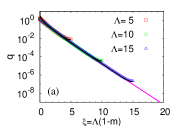
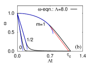
Figure 4: (a) Numerical solutions of Eq. (9) (symbols) and the corresponding “bulk solutions” $q_{b}(\xi)$ (lines) for $\Lambda=5,10,15$. (b) The implicit solution (10) (the blue lines) versus the numerical solution of the $\omega$-equation (the black lines) for $\Lambda=8.0$ at three Lagrangian points: $m=0,0.5$ and $1.0$. The red straight line shows the smoothly matched asymptotic separable solution at $m=1$ (b).

Early dynamics and collapse time. To find the collapse time $t_{c}$ [a free parameter in the separable solution (5)], one needs to solve the $\omega$-equation with a given initial condition. In general, this can only be done numerically. We obtained analytic estimates of $t_{c}$, separately for small and large $\Lambda$, for $\omega(m,t=0)=1$.

For $\Lambda\ll 1$ the separable solution (5) and (7) is valid, at order $\Lambda^{2}$, at any $t\geq 0$. This yields the leading-order estimate $t_{c}\simeq 2\Lambda^{-2}$. For $\Lambda\gg 1$ the initial stage of the cooling dynamics should be addressed separately. We notice that at early times the term $\xi\partial^{2}_{\xi}\omega$ in Eq. (8) is small compared to the rest of terms. With this term neglected Eq. (8) reduces to a first-order equation, $\omega\partial_{\tau}\omega-\partial_{\xi}{\omega}=-\xi\omega$, which is soluble by characteristics. The solution $\omega(\xi,\tau)$, in an implicit form, is

$$\sqrt{2}\,e^{-\xi^{2}/2}\omega(\xi,\tau)\int_{\xi/\sqrt{2}}^{\sqrt{\frac{\xi^{2}}{2}-\ln[\omega(\xi,\tau)]}}e^{z^{2}}\,dz=\tau\,;$$ (10)

it is depicted, at points $m=0,1/2$ and $1$, in Fig. 4b. At $\xi\gg 1$ (where most of the gas is located), Eq. (10) predicts an early-time asymptote $\omega(\xi,\tau\ll 1)=1-\xi\tau$ which can be also obtained directly from Eq. (8) with the heat conduction neglected completely. The “bottleneck” of cooling, however, is at large heights, $\xi\ll 1$, where the gas is very dilute. An early-time asymptote there, as predicted from Eq. (10), is

$$\omega\simeq 1-\xi\tau-\tau^{2}/2=1-\Lambda^{2}(1-m)t-\Lambda^{2}t^{2}/2\,.$$ (11)

The implicit solution (10) breaks down, at a given $\xi$, at time $\tau\sim\mbox{min}\,(1,\xi^{-1})$, and then the full $\omega$-equation must be solved. Eventually, as $\tau$ approaches $\tau_{c}$, the separable solution (5) emerges.

We stress that, at $\Lambda\gg 1$, the cooling process is highly nonuniform, see Fig. 5a and b. For example, at $m=0$ a rapid initial decay $\omega=1-\Lambda^{2}t$ crosses over, after a short time $t\sim\Lambda^{-2}$, into a very slow decay $\omega=\Lambda q(\Lambda)(t_{c}-t)$, as $q(\Lambda)$ is exponentially small. Meanwhile, at $m=1$ a slow initial decay $\omega=1-\tau^{2}/2$ crosses over into a rapid decay $\omega=q_{0}(\tau_{c}-\tau)$. At $t=t_{c}$ $\omega$ vanishes at all $\xi$ (that is, at $y=0$). Note that the dynamics at $m=1$ are independent of $\Lambda$ in the stretched time $\tau=\Lambda t$

A good estimate of the collapse time $\tau_{c}$ at large $\Lambda$ can be obtained by matching, at $\xi=0$, the late-time asymptote $(\tau_{c}-\tau)q_{0}$ with the early-time solution (10), see Fig. 4b. This yields an algebraic equation for $\tau_{c}$:

$$\left[(\pi/2)^{1/2}{\rm erfi}(2^{-1/2}\tau_{c}^{-1})+q_{0}^{-1}\right]=\tau_{c}\exp[1/(2\tau_{c}^{2})]$$ (12)

which has a unique solution $\tau_{c}\simeq 1.10$, or $t_{c}\simeq 1.10\Lambda^{-1}$. For comparison, a numerical solution of Eq. (8), for large $\Lambda$, with the initial condition $\omega(\xi,t=0)=1$ yields $\tau_{c}=1.145$ which agrees with our estimate to about $4\%$. The slope of the collapsed curves $\omega(\xi=0,\tau)$ for large $\Lambda$ (Fig. 4b) near $\tau=\tau_{c}$, $\partial_{\tau}\omega(\xi=0,\tau_{c})=1.624$, is in very good agreement with the asymptotic value $q_{0}=1.633356$.

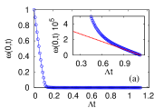
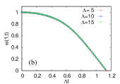
Figure 5: (a) $\omega(m=0,t)$ at $\Lambda=10$. The inset shows a blow-up near $\tau_{c}$, and the asymptote $(\tau_{c}-\tau)q(\Lambda)$ (the red dashed line). (b) $\omega(m=1,t)$ vs. $\tau=\Lambda t$ for $\Lambda=5,10,15$ collapse into a universal curve.

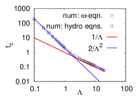
Figure 6: The collapse time versus $\Lambda$. Numerical results from the $\omega$-equation and from the full hydrodynamic equations (1)-(3) with $\varepsilon=0.025$ are shown by symbols, the small- and large-$\Lambda$ asymptotes are denoted by lines.

Our predictions of the $\Lambda$-dependence of $t_{c}$ are summarized in Fig. 6. The small- and large-$\Lambda$ asymptotes are in excellent agreement with numerical results. Returning to the dimensional units, we observe that, at $\Lambda\ll 1$ the collapse time $t_{c}$ is much longer than the heat diffusion time. At $\Lambda\gg 1$ $t_{c}$ is of the order of $(\varepsilon\Lambda)^{-1}t_{f}\sim(1-r^{2})^{-1/2}t_{f}$ which, for nearly elastic collisions, is much longer than the free fall time $t_{f}$.

Having found $\omega(\xi,\tau)$ we can find the rest of hydrodynamic fields. Here we present the results for $\Lambda\gg 1$. In the early stage of cooling the gas density is $n(\xi,\tau)=(\xi/\Lambda)(1-\xi\tau)^{-2}$ and velocity $v(\xi,\tau)=\Lambda(\Lambda-\xi)[(\Lambda+\xi)\tau-2]$. Close to collapse the density $n(\xi,\tau)=\xi(\tau_{c}-\tau)^{-2}\,q^{-2}(\xi)$ blows up as $(\tau_{c}-\tau)^{-2}$. The gas velocity is $v(\xi,\tau)=-2\Lambda(\tau_{c}-\tau)\int_{\xi}^{\Lambda}[q^{2}(\xi^{\prime})/\xi^{\prime}]\,d\xi^{\prime}$. At $\tau<\tau_{c}$ it diverges logarithmically at $\xi=0$ (that is, linearly at $y\to\infty$), but vanishes everywhere at $\tau=\tau_{c}$, while the mass flux $nv$ blows up at $\tau=\tau_{c}$. Going back to Eulerian coordinate $y=(\tau_{c}-\tau)^{2}\int_{\xi}^{\Lambda}[q^{2}(\xi^{\prime})/\xi^{\prime}]\,d\xi^{\prime}$, we see that the velocity field is simply $v(y,t)=-2y/(t_{c}-t)$.

Summary. Our MD simulations and hydrodynamic theory depict a coherent picture of thermal collapse which develops in the process of a free cooling of a granular gas under gravity. One of the signatures of this picture is the universal scaling behavior of the total energy $E(t)\sim(t_{c}-t)^{2}$ as $t\to t_{c}$.

It would be interesting to test the quantitative predictions of our theory in experiment. A possible experiment can employ metallic spheres rolling on a slightly inclined smooth surface and driven by a rapidly vibrating bottom wall, like in Ref. Kudrolli . After the “granular gas” reaches a steady state, one stops the driving and follows the cooling dynamics with a fast camera and a particle tracking software. While particle rotation and rolling friction may prove important, we expect that the main predictions of the theory, including the scaling behavior of the total energy at $t\to t_{c}$, will persist.

LT and DV are grateful to the U.S. Department of Energy for financial support (Grant DE-FG02- 04ER46135). BM acknowledges support from the Israel Science Foundation (grant No. 107/05) and from the German-Israel Foundation for Scientific Research and Development (Grant I-795-166.10/2003).

References

- (1) P.K. Haff, J. Fluid Mech. 134, 401 (1983).
- (2) J. J. Brey, J. W. Dufty and A. Santos, J. Stat. Phys. 97, 281 (1999); I. Goldhirsch, Ann. Rev. Fluid Mech. 35, 267 (2003); N.V. Brilliantov and T. Pöschel, Kinetic Theory of Granular Gases (Oxford University Press, Oxford, 2004), and references therein.
- (3) D.C. Rapaport. The Art of Molecular Dynamics Simulation (Cambridge University Press, Cambridge, 2004).
- (4) In experiment, an (almost) isothermal initial state is easily realized when the particle density and the inelasticity are not too large, see e.g. Ref. Kudrolli .
- (5) Granular hydrodynamics assumes scale separation, which often demands nearly elastic collisions Goldhirsch+BP .
- (6) As the gas approaches collapse, a close-packed “condensate” forms, where the dilute gas model breaks down. Therefore, it might seem surprising that it describes the kinetic energy history remarkably well, see Fig. 2a, until the time of collapse. The reason is that the kinetic energy of the condensate particles is extremely small, and the main contribution to the energy comes from the gas particles.
- (7) Y. Bromberg, E. Livne, and B. Meerson, in Granular Gas Dynamics, T. Pöschel and N. Brilliantov (eds.), Springer, 2003, p. 251.
- (8) In the expression for the heat flux we omitted a term with the density gradient Goldhirsch+BP . It can be neglected in the nearly elastic limit.
- (9) J. G. Blom and P. A. Zegeling, Trans. Math. Software 20, 194 (1994).
- (10) We checked that the -equation predicts a finite-time collapse for other initial states as well, e.g. when starting from a (non-isothermal) steady state bromberg03 , corresponding to a “thermal” bottom.
- (11) A. Kudrolli, M. Wolpert, and J.P. Gollub, Phys. Rev. Lett. 78, 1383 (1997); D. Blair and A. Kudrolli, Phys. Rev. E 67, 041301 (2003).