Limits of the equivalence of time and ensemble averages in shear flows.

Abstract

In equilibrium systems, time and ensemble averages of physical quantities are equivalent due to ergodic exploration of phase space. In driven systems, it is unknown if a similar equivalence of time and ensemble averages exists. We explore effective limits of such convergence in a sheared bubble raft using averages of the bubble velocities. In independent experiments, averaging over time leads to well converged velocity profiles. However, the time-averages from independent experiments result in distinct velocity averages. Ensemble averages are approximated by randomly selecting bubble velocities from independent experiments. Increasingly better approximations of ensemble averages converge toward a unique velocity profile. Therefore, the experiments establish that in practical realizations of non-equilibrium systems, temporal averaging and ensemble averaging can yield convergent (stationary) but distinct distributions.

A central tenant of statistical mechanics is the ergodic hypothesis: during time evolution, thermodynamic systems pass through almost all possible microstates leading to the equivalence of time and ensemble averages Boltzmann (1871, 1895a, 1895b); Landau and Lifshitz (1980); Pathria (1996). The exploration of phase space is achieved through thermal fluctuations, and this allows for a description of equilibrium dynamics in terms of well defined averaged observables. The observables are extracted either by averaging over states explored over long periods of time or from ensembles of states distributed over all of phase space, whichever method is most convenient for the observable being studied. A natural questions is whether or not athermal fluctuations in a driven system lead to the equivalence of time and ensemble averages through a similar exploration of phase space. Ideally, testing the equivalence of time and ensemble averages in driven systems requires measuring the instantaneous value of an observable for an infinite period of time (temporal averages) and constructing an infinite number of ensembles (ensemble averages). This is untenable for real experiments; however, if time scales of observation are faster than intrinsic timescales, it is possible to gather a reasonable approximation of the distribution of values for an observable.

The averaging process is governed by the fluctuations that move the system through phase space. In driven, complex fluids, athermal fluctuations arise through particle rearrangements that are induced by flow. The potential for these athermal fluctuations to play a role that is similar to thermal fluctuations in normal fluids is the basis of many statistical treatments of highly non-equilibrium complex fluids Cugliandolo et al. (1997); Ono et al. (2002); Berthier and Barrat (2002); Zamponi et al. (2005). A specific example of this are the various proposals for using effective temperatures Cugliandolo et al. (1997); Ono et al. (2002); Berthier and Barrat (2002) in driven systems. An open question in this field is the quantitative disagreement O’Hern et al. (2004) between different definitions of effective temperatures Zamponi et al. (2005). These disagreements may be connected to the ability of athermal fluctuations to provide sufficient exploration of phase space for certain variables, such as velocity. In this letter, we specifically focus on the ability of athermal fluctuations in the system to explore phase space in a manner that results in an equivalence between time and ensemble averages. Testing such an equivalence is an important step in understanding how well the various elements of statistical mechanics (such as temperature) can be translated to driven systems.

In considering any comparison of time and ensemble averages, it is important to recognize the separate question of the convergence of either time or ensemble averages. Independent of whether the two averages agree, it is possible that the nature of athermal fluctuations in a driven system are such that average quantities are not well-defined on experimentally accessible time scales or number of ensembles. This is highlighted by work in granular matter in which extremely long times were required for convergence of the average density under tapping Nowak et al. (1998). As we will demonstrate, for our system, both the time and ensemble averages are well-defined.

In this Letter, we report on measurements of the average velocity profile using a model two-dimensional foam: a bubble raft Bragg and Lomer (1949). One advantage of this system is the irrelevance of thermal fluctuations due to the macroscopic nature of the bubbles. Instead, the fluctuations are the result of bubble rearrangements during flow Weaire and Hutzler (1999). Even though the average velocity profile for foam has been the subject of substantial theoretical Varnik et al. (2003); Xu et al. (2005); Kabla and Debrégeas (2003); Weaire et al. (2006) and experimental Coussot et al. (2002); Lauridsen et al. (2004); Debrégeas et al. (2001); Gopal and Durian (1999); Rouyer et al. (2003); Dollet et al. (2005) work, the connection between time and ensemble averages for velocity profiles remains an open question.

The bubble raft is produced by flowing regulated nitrogen gas through a needle into a homogeneous solution of 80% by volume deionized water, 5% by volume Miracle Bubbles (from Imperial Toy Corporation), and 15% by volume glycerine. The glycerine provides additional stabilization of the bubble raft as a function of time. The bubbles are confined between two parallel bands separated by a distance $d=57\ {\rm mm}$. The bands are driven at a constant velocity $v_{w}$ in opposing directions. This applies a steady rate of strain to the system given by $\dot{\gamma}=2v_{w}/d=1.4\times 10^{-3}\ {\rm s^{-1}}$. The total applied strain is $\gamma=\dot{\gamma}t$, where $t$ is the time interval under consideration. The direction of flow imposed by the bands is taken to be parallel to the x-axis. We use a CCD camera to capture the state of the system at a frame rate of $10\ {\rm Hz}$. A Particle Image Velocimetry program piv is then used to extract velocities of individual bubbles using consecutive images. Each consecutive pair of images corresponds to a measurement of its instantaneous velocity. For this paper, we focus exclusively on the behavior of the velocity in the x-direction, and the system was divided into forty bins in the y-direction so as to measure the velocity as a function of y. The bubbles are relatively monodisperse, with a bubble diameter of $D=2.66\pm 0.2\ {\rm mm}$. Details of the apparatus and methods can be found in Ref. Wang et al. (2006a).

The results presented in this letter are based on thirty different experimental realizations of a bubble raft. All of the parameters for each experimental realization were the same except for the configuration of the bubbles. In each of the experimental realizations, the system is subjected to a total strain of five and $N=1000$ consecutive images of the bubbles are captured. From these thirty different experimental realizations, we develop two different data sets: a time set and an ensemble set. The time set is the 30 independent time series of the bubble velocities. A member of the time set corresponds to a single experimental realization with $1000$ elements. Each element captures the instantaneous position and velocity of the bubbles as measured between successive images at a given time (or value of strain). A member of the “ensemble set” is constructed from the thirty experimental realizations by randomly sampling $1000$ elements from the thirty experimental realizations. We build 30 such members to constitute the ensemble set. This procedure ensures an equal number of elements in each of the members of the time and ensemble sets. This allows for a direct statistical comparison between the two data sets. A time/ensemble average refers to averaging all instantaneous velocities from a individual member of the time/ensemble set of data.

To characterize the system’s behavior, we measured the distribution of velocities, the time-correlation of the velocities, the average velocity profiles, and characterized the convergence rate of the averaging process. All of these studies (except the velocity correlations) were made for both the time and ensemble data sets. The results for the velocity distributions are shown in Fig. 1 for a single member of both the time and ensemble set. Sampling the velocities from either time sets Wang et al. (2006b) or ensemble sets result in a Lorentzian distribution. However, as we will show, a key distinction lies in the distribution of the mean values for different members of the respective sets.

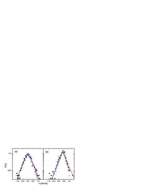
Figure 1: (color online) The probability distribution of velocities is indicated for ensemble averaging (open circles) and time averaging (closed squares). The solid lines are Lorenztian fits to the data, red curves for time averaged data and blue for ensemble averaged data. (a) Results for a position at the center of the trough. For the ensemble (time) average the center of the Lorentzian fits are at $0.01\pm 0.01$ ($-0.01\pm 0.01$) and the widths are $0.68\pm 0.02$ ($0.72\pm 0.02$), respectively. (b) For a position $0.25d$ from the center. For the ensemble (time) average the center of the Lorentzian fits are at $0.41\pm 0.01$ ($0.36\pm 0.01$) and the widths are $0.47\pm 0.03$ ($0.52\pm 0.02$), respectively.

The average velocity profiles are approximately linear Wang et al. (2006a). To characterize the relative deviations of the various velocity profiles in different sets, Fig. 2 plots the difference between the individual average velocity profiles and the mean profile ($v_{m}$) for ten members of the time set and ten members of the ensemble set. In the case of time averaging, the resulting average velocity profiles qualitatively differ from each other and exhibit relatively (compared to the ensemble profiles) large deviations from the mean. In contrast, the ensemble averages are essentially indistinguishable from each other (this is quantified by the standard deviation between profiles, see Fig. 2).

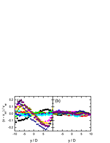
Figure 2: (a) Deviation of time average velocity profiles (normalized by the wall speed $v_{w}$) from the mean profile ($v_{m}$) generated by ten members of the time set. (b) Deviation of ten different ensemble averages of the velocities from the mean profile. Plotting the deviation highlights the differences between the different time average profiles. The average standard deviation for time average profiles in (a) is $0.081$, in contrast, the ensemble averages shown in (b) are relatively indistinguishable with a standard deviation of $0.017$. The y-position is scaled by the bubble diameter $D$.

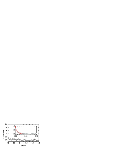
Figure 3: This is the decay in the correlation of the mean velocity $0.25d$ away from the trough center. The total strain in each experiment is $5$, and we only show the autocorrelation to a unit strain to make it visually easier to read. The remainder of the curve is qualitatively unchanged at higher strains. The inset shows a closeup at short strain along with an exponential fit (correlation $\propto\exp(-\gamma/0.01)$.

There are two key issues regarding the average profiles: (1) are they computed over independent configurations? and (2) have the averages converged? Fig. 3 and 4 address these two questions. In Fig. 3, the autocorrelation of instantaneous velocities for a member of a time set and an exponential fit to the correlation function ($\propto\exp(-\gamma/0.01)$) are shown. The decay constant corresponding to a strain of 0.01 is consistent with the previously reported yield strain in polydisperse bubble rafts ($\sim 0.05$) Dennin (2004). As the yield strain corresponds to the point at which elastic response gives way to flow through significant bubble rearrangements, it is reasonable that this determines the interval of strain necessary to produce independent configurations. Therefore, time averages using a total strain of 5 consist of between 100 to 500 independent configurations. While building an ensemble member, we randomly choose states of velocity configurations across all thirty members of the time set. This results in the average strain between randomly chosen states being 0.15, with a correlation less than the baseline noise in Fig. 3. The selection of these states across 30 independent time members, further decreases any correlations between them.

We find the rate of convergence to the mean value of the velocity profile is the same for members of the time and ensemble sets. However, the distribution of final mean values attained are different, with the time set showing a significantly larger spread in the converged mean values than those from the ensemble set. In Fig. 4, the convergence of the mean velocity as a function of the number of bubbles used to compute the average is plotted for ten members of the time and ensemble averages. Plotting the mean velocity versus the number of bubbles allows for direct comparison of the time and ensemble averages. However, it should be noted, that for the time averages, the number of bubbles corresponds directly to increasing time, or strain, which in this case is a strain $\leq 5$. In all cases (ensemble and time averages), the mean values converge to a well-defined value after averaging over approximately $n=2000$ bubbles. (This corresponds to a strain of 1 for the time averages, or approximately 100 independent configurations, and is consistent with previous measurements of the rate of convergence Lauridsen et al. (2004)). The spread in the final mean values is very different for the two sets. For the time averages, as expected from Fig. 2, the deviation in final mean values is larger than the fluctuation in the mean for large enough values of $n$. For the ensemble averages, the deviation in final mean values is similar to the fluctuation in the mean. To quantify this deviation, for a given set of average velocities, we define the deviation $\delta\equiv v_{max}-v_{min}$, where $v_{max}$ ($v_{min}$) is the largest (smallest) final average velocity in the set.

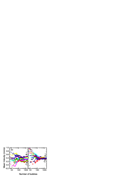
Figure 4: (color online) The mean values of the velocity $0.25d$ from the center as a function of the number of bubbles used to compute the average for (a) time averaging and (b) ensemble averaging. For illustration purposes, 10 of the 30 runs are shown. The deviation in the final values (indicated by the arrows and $\delta$) is larger for time averages than ensemble averages. When we use the complete set of 30 runs, we obtain $\delta=0.258{\rm mm/s}$ for time averages and $\delta=0.052{\rm mm/s}$ for ensemble averages.

Figure 5: (color online) Plot of the average deviation $<\delta(M)>$ between different ensemble averages as a function of $M$, the number of runs used to generate the ensemble set. As the number of independent runs used to generate the ensemble increases, the deviation between computed averages decreases.

Next, in Fig. 5 we describe the spread in the final mean values of the velocity profile parameterized by $\delta$ as a function of an increasing number of independent members of the time set, $M$, used in constructing the ensemble set. This is done to test whether or not thirty independent members of the time set is sufficient to build an ensemble set with physical relevance, i.e. uncorrelated and independent. One method of testing this is to consider ensembles constructed from constructed $M<30$ members of the time set, and measure $\delta(M)$. To increase the statistics, a number of ensemble sets are generated for each $M<30$, and one considers $<\delta(M)>$ over these sets. Figure 5 is a plot $<\delta(M)>$ for each $M$, and it confirms our expectation that increasing $M$ should increase the independence between the randomly selected velocities, resulting in a better approximation of an ensemble average. For $M\geq 20$, the value of $<\delta(M)>$ is bounded within range of the error bar of the value at $M=20$. This has two important consequences. First, the independence of $<\delta(M)>$ on $M$ for $M\geq 20$ is strong evidence that thirty independent experimental realizations provides a sufficient approximation of the ensemble average for this system. Second, the indication that $<\delta(M)>$ has converged to a nonzero value may be attributed to the finite size of the system. An interesting future study will be the dependence of $<\delta(M)>$ as a function of the system size.

We have presented three main results. First, athermal fluctuations generated during the flow of a bubble raft are sufficient to produce stationary, time-averaged velocity profiles after a total strain of approximately one (Fig. 4). Second, these fluctuations do not provide sufficient exploration of phase space to result in a unique time-average. In other words, different realizations of a bubble raft produce different time-averaged velocity profiles that exhibit a measurable and significant deviation from each other (see Fig. 4 and 2). Third, by sampling velocities from different realizations of the experiment, the resulting ensemble averages demonstrate a convergence towards similar velocity profiles (Fig. 4 and 2). Putting these results together, one concludes that the limit of time averaging is different from that of ensemble averaging for this system in at least one crucial aspect i.e., there is no convergence to a unique time-average for all experimental realizations of the bubble raft, but the ensemble averages converge to final velocity profiles that are consistent with a unique profile.